Kalman Filter-Based CNN-BiLSTM-ATT Model for Traffic Flow Prediction

1  Introduction

Recently, with the rise of people’s demand for cars and the development of new energy vehicles, the number of private cars has increased rapidly. Until September 2022, the number of cars in 72 cities nationwide reached 315 million, and the vast number of cars has brought enormous pressure on urban road traffic. The service level of urban roads is an essential reflection of the country’s economic development. As an essential part of urban road traffic, the operation efficiency of highways affects the country’s economic level and people’s quality of life. Therefore, the prediction of traffic flow by analyzing the data obtained from monitors on highways is the research direction of many scholars today. A large number of methods have been cited, such as the early traditional linear forecasting method, which is relatively simple in its operation steps but cannot reflect the traffic flow state accurately because it fluctuates from moment to moment [1]. The current traffic flow prediction models are mainly divided into four categories: statistical theory models, nonlinear theory models, intelligent theory models, and combined models. Statistical theory models, including the standard Kalman filter prediction models [2]; nonlinear theory models, such as wavelet theory models [3] and chaos theory models; intelligent theory models, such as Machine learning models [4] and neural network models [5]; combined models, such as Deep learning combined models [6], Machine learning combined models, and Deep learning and Machine learning combined models [7]. This experiment uses the Deep learning combined model.

Traffic flow can be divided into long-term, medium-term, and short-term predictions according to the length of the forecast time. Long-term prediction mainly refers to the traffic flow prediction for the selected areas for one year or even for the next few years; medium-term prediction mainly predicts the traffic flow for three time periods: weekly, daily, and hourly; while short-term prediction mainly predicts the real-time traffic flow for the specified road section for the next fifteen minutes [8–10]. This experiment investigates short-term traffic flow prediction.

Short-term traffic flow prediction is affected by unexpected accidents, which has high requirements on the prediction model, and how to handle the distinctive values becomes the key to prediction [11]. In this paper, a CNN-BiLSTM-Attention traffic prediction model based on Kalman filter data processing is proposed, which can cope with traffic flow data under different conditions and achieve better experimental results. This model consists of three main parts:

(1)   Convolutional Neural Networks (CNN): Responsible for extracting spatial feature vectors and dimensionality reduction of data [12].

(2)   Bi-directional Long Short-Term Memory (BiLSTM): It comprehensively analyzes sequence information by forward LSTM and backward LSTM, then extracts temporal features.

(3)   Attention Mechanism: Different weight coefficients are assigned to different features, then these weight coefficients are weighted for the output results [6].

The remaining sections of this paper are organized as follows: in Section 2, the research of some scholars in the field of intelligent traffic flow prediction in recent years is reviewed; in Section 3, the preprocessing of experimental data is introduced; in Section 4, the primary model used in this experiment is introduced; in Section 5, the training process of the model and the experimental results obtained are presented; in Section 6, the experimental conclusion is given.

2  Related Work

After entering the 21st century, computer science and technology have developed rapidly. Artificial intelligence has been applied to all aspects of life, and more intelligent traffic prediction methods have emerged, for example, various prediction methods based on Machine learning and Deep learning have been cited by many scholars [13]. When the amount of data is small, the performance of Machine learning is better than that of Deep learning and the execution time is shorter [14], while Deep learning requires a large amount of data for training and takes longer time, so the application scenarios of both are also different [15].

Feng et al. [16] proposed an Adaptive Multicore Support Vector Machine (AMSVM) prediction model based on spatio-temporal correlation, which fuses Gaussian kernel functions with polynomials and optimizes model parameters using an adaptive particle swarm algorithm. The fused model can automatically adjust the weights of relevant parameters according to real-time traffic flow changes, and then combine spatio-temporal information for traffic flow prediction. Luo et al. [17] proposed a hybrid forecasting method integrating Discrete Fourier Transform (DFT) and Support Vector Regression (SVR) for holiday traffic forecasting, using the DFT method and setting thresholds to extract trend features in traffic flow data, SVR was used to analyze the residual components, and finally, the trend information and residual values were used to forecast the traffic flow. Ma et al. [18] combined Machine learning with statistics and post-processed the results by Autoregressive Integrated Moving Average (ARIMA) analysis to improve prediction accuracy.

In the meantime, Deep learning techniques have been developed in traffic flow prediction. Fukuda et al. [19] proposed a Deep learning model combining graphical convolutional networks with traffic accident information features to obtain a large amount of traffic data by setting up various traffic accident scenarios for simulation and using these data for model training, and the final model obtained can be helpful in traffic flow prediction. Impedovo et al. [20] proposed a Deep learning architecture Traffic Wave for time series analysis inspired by Google DeepMind’s Wavenet network and applied it to traffic flow prediction. Kong et al. [21] used a Restricted Boltzmann Machine (RBM) based on Deep learning architecture as a method for traffic flow prediction. They used the RBM model to the model has better results in training traffic flow samples, unlike external neural networks. Chen et al. [22] proposed a Fuzzy Deep learning method (FDCN) to predict traffic flow, which is built on fuzzy theory and the Deep residual convolutional network model, and its main idea is to introduce fuzzy theory into the Deep learning model to reduce the impact caused by data uncertainty. Whether Machine learning or Deep learning, the results are always poor when only one method is used for prediction, so people integrate different methods to complement their functions. Xiao et al. [23] proposed a hybrid Long Short-Term Memory (LSTM) neural network with more accurate predictions than the regular LSTM model. Jiang et al. [24] summarized the application of Graph Neural Networks (GNN) in traffic flow prediction in recent years. Ye et al. [25] offered many traffic flow prediction models combining GNN and Deep learning that can address various traffic challenges.

The above literature reviews the applications of Machine learning and Deep learning in traffic flow prediction in recent years [26–28]. Since the traffic flow data is vast and complex and not stable, how to process the raw data becomes the primary prerequisite for prediction [29]. The method proposed in this paper can cope with various complex data and has a broader scope of application.

3  Data Pre-Processing

Because the highway data involves national machinery and security, it is not appropriate to use the data from the last three years. The PEMS04 data set used in this experiment is from the California highway network, which is obtained from the California highway traffic flow data obtained from 307 detectors for 58 consecutive days starting from January 1, 2018, and collected every 5 min. All the traffic flow data obtained are plotted into a waveform graph. As shown in Fig. 1, by observing the graphs, the traffic flow data for each week has a similar trend, and the traffic flow was the largest on February 2, 2018, and the smallest on February 4, 2018.

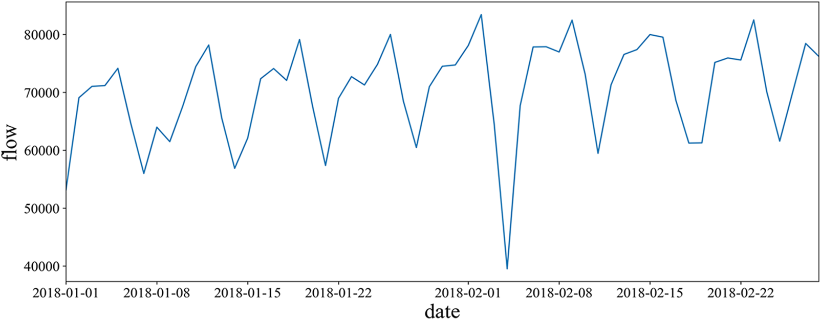
Figure 1: Total traffic flow waveform

The traffic volumes for each hour of the day are plotted as box plots in Fig. 2. From the distribution of the box plots, it can be observed that there are different levels of outliers for most hours of the day.

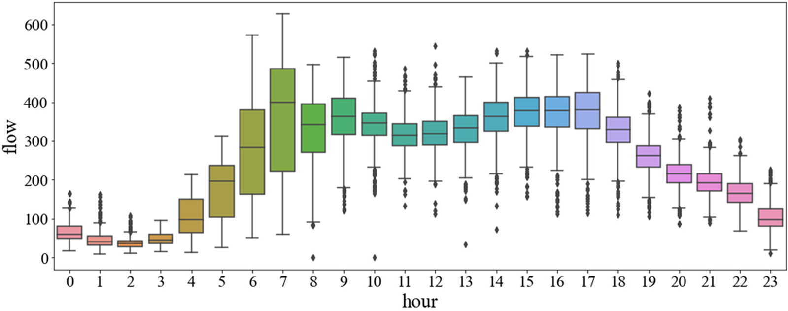
Figure 2: One-day traffic distribution box chart

3.1 Feature Visualization

The three main feature parameters of this experimental data are flow, occupancy, and speed [30]. To improve the accuracy of the model, this experiment also extracted the information of hours, minutes, days of the month, days of the week, and months, and added the first-order differential and second-order differential data of traffic flow. The correlation coefficients are represented by heat maps, as in Fig. 3. From the heat map, it can be seen that the vehicle speed shows a negative correlation with flow and occupancy, and the correlation between occupancy and traffic is strong. The darker the color, the closer the correlation coefficient is to 1. The correlation coefficients of flow with occupancy and speed are 0.68 and 0.30, respectively. The correlation coefficients between different feature parameters are calculated using Pearson’s correlation coefficient calculation method, and the feature parameters with correlation coefficients greater than 0.05 are selected, which are: flow, occupancy, speed, hour, day of the week, month, first-order differential, and second-order differential data. Feature visualization can view the data distribution and show the variability between different features.

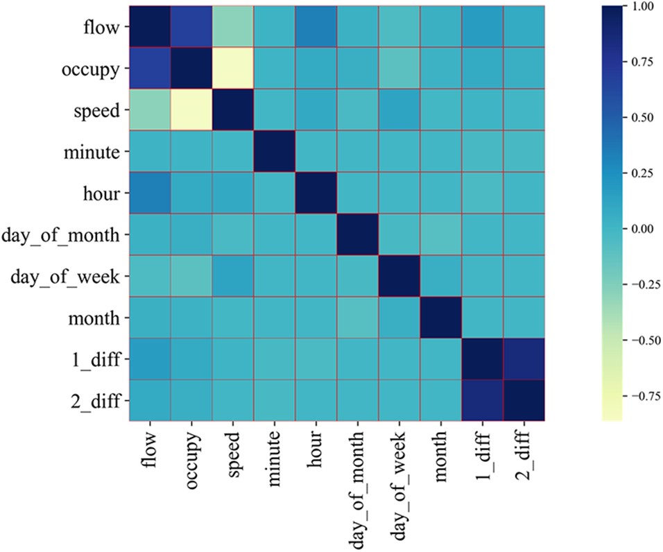
Figure 3: Correlation coefficient heat map

3.2 Kalman Filtering

The Kalman filter is widely used in various fields, such as communication systems, aerospace, industrial control, etc. The core idea of the Kalman filter is state estimation, which helps to understand and control the system. It can estimate and predict the operation state of the system in real-time, so the Kalman filter has not only the function of filtering but also the function of prediction. However, the general Kalman filter model is less accurate in short-time traffic flow prediction, so this experiment only uses the Kalman filter to process the data [2].

Due to the interference of external factors, the traffic flow data was found to be too volatile when plotted, so the traffic flow data was subjected to Kalman filtering. Data filtering is generally the process of removing the noise generated by external disturbances to restore the authenticity of the original data. Kalman filtering is inputting the data into the time update equation and state update equation, updating the state quantities in real time, and finally giving an optimal estimate of the results. The Kalman filter time update equation is Eqs. (1) and (2).

x^k¯=Ax^k−1+Buk−1(1)

Pk¯=APk−1AT+Q(2)

Its state update equation is Eqs. (3)–(5).

Kk=Pk¯HTHPK¯HT+R(3)

x^k=x^k¯+K(zk−Hx^k¯)(4)

Pk=(I−KkH)Pk¯(5)

The fluctuation of the data after the Kalman filtering process becomes significantly smaller, as shown in Fig. 4. Although the processing result may lose the specificity of the original data to some extent, reducing the fluctuation of the data does make the prediction results more accurate.

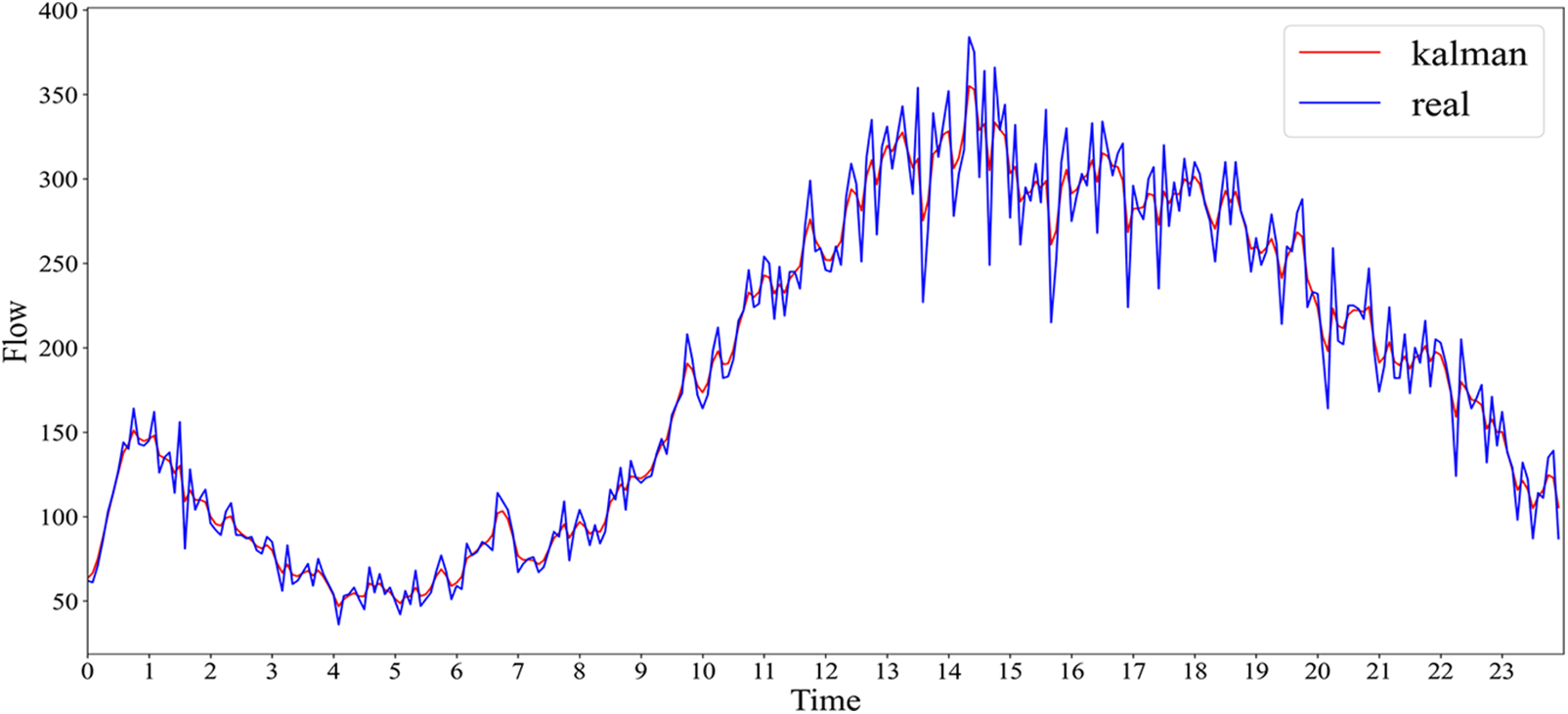
Figure 4: Passes through the car flow data after Karman filtering

3.3 Normalization Process

The filtered data will be normalized, and this experiment uses the maximum-minimum normalization method commonly used for data normalization to facilitate the model input later. It can be defined as Eq. (6).

x′=xi−xminxmax−xmin(6)

Finally, the training set and the test set are divided, the data from 51 consecutive days from January 1 to February 20 are taken as the training set. The data of the last seven days from February 21 to February 27 are taken as the test set.

4  Predictive Model Building

When conducting traffic flow prediction experiments, three basic feature parameters cannot be ignored, they are flow, occupancy, and speed, and the essence of traffic flow prediction is to predict the traffic flow in the following period by these three parameters because the short-term traffic flow prediction is more dependent on the feature parameters. This experiment adds five new parameters to the primary feature parameters, which are hour, day of the week, month, first-order difference, and second-order difference, so there are eight feature parameters in this experiment.

4.1 CNN Model

Through research and experiments, it is found that the prediction results are better when the convolutional neural network layer is used as the input layer of the model. Generally, CNN consists of an input layer, a convolutional layer, a pooling layer, and a fully connected layer. After the data is input by the input layer, the convolutional layer extracts the data feature information, and the pooling layer selects these features to reduce the number of variables in the feature map, thus reducing the computation and improving the computation efficiency. From the pooling layer to the fully connected layer, the data is mapped from more to less, and dimensionality reduction is performed to facilitate the processing of the data [31].

In this paper, a one-dimensional CNN is used to enable feature extraction of time series. Known sequence: A={a0,a1,a2,…,am}, L(A)=m+1,B={b0,b1,b2,…,bk},L(B)=K+1, C represents the new sequence obtained after the convolution operation of two sequences A and B, the calculation formula is Eqs. (7) and (8).

C=A∗B=a0bn+a1bn−1+⋯+an−1b1+anb0=∑akbn−k(7)

L(C)=L(A)+L(B)−1(8)

CNN extracts the features of a time series, which is to find a sequence of length m as a filter, and the original time series do convolution, pooling, and other operations to get the deep sequence representation. This experiment sets the number of CNN convolutional layers to 1 and the activation function uses the ReLu function. The ReLu function is not only computationally simple but also ensures the non-negativity of the traffic flow data and accelerates the convergence speed.

4.2 BiLSTM Model

Unlike the convolutional neural networks that deal with local spatial feature information, recurrent neural networks (RNN) are used to analyze time series information. Due to the limited memory of traditional RNN, they cannot solve the long-term dependence problem, if this time series is too long, the influence of the information source from the beginning to the end of the network structure will gradually weaken, which gives rise to the gradient disappearance problem. The long short-term memory network model was created to solve this problem. Compared with the traditional RNN model, the LSTM model is much more complex in structure, mainly by adding three controllers: input gate, forgetting gate, and output gate. The input gate obtains external information; the forgetting gate decides whether to forget the information in the neuron cells selectively; the output gate is responsible for outputting the current state information. The unique “gate” structure is an excellent solution to the problem of gradient disappearance and gradient explosion in the traditional RNN model when dealing with long sequences. Its memory is better [32]. The neural network structure of LSTM is shown in Fig. 5a, and the principal equation is shown in Eqs. (9)–(14).

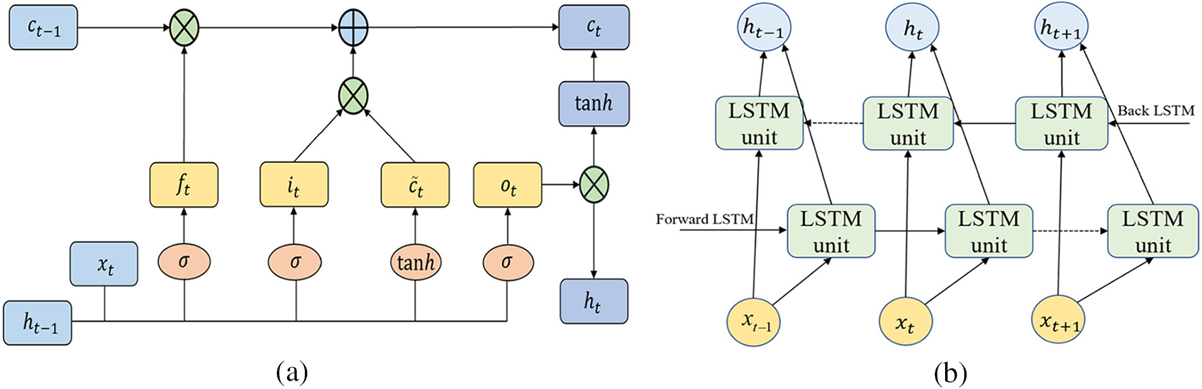
Figure 5: Neural network structure of LSTM and BiLSTM (a) LSTM, (b) BiLSTM

ft=σ(Wf⋅[ht−1,xt]+bf)(9)

it=σ(Wi⋅[ht−1,xt]+bi)(10)

ct=ft∘ct−1+it∘c~t(11)

c~t=tan⁡h(WC⋅[ht−1,xt]+bc)(12)

ot=σ(Wo⋅[ht−1,xt]+bo)(13)

ht=ot∘tan⁡h(ct)(14)

Both RNN and LSTM predict the output of the next moment from the previous information, which cannot capture the dependence of bidirectional information, resulting in the inability to reasonably predict the state value of the current moment in dealing with some specific problems. The bi-directional LSTM can take into account both forward and backward information. For each moment, the system will provide the input to two LSTMs with the same structure but opposite directions, which accurately determine the output of the current moment by combining the before and after information, and thus are more suitable for handling long sequence tasks with bidirectional dependencies. The bi-directional LSTM is composed of two unidirectional LSTMs with identical algorithms, and its neural network structure is shown in Fig. 5b. In this experiment, the number of neurons of BiLSTM is set to 40, and the activation function adopts the tanh function, which improves the convergence speed compared with the sigmoid function [23].

The forward propagation layer and the backward propagation layer each make a nonlinear change of the input data to obtain the hidden output layer, and the two independent hidden layers are then combined and output to the same output layer through a layer of connection. The formula is expressed as Eqs. (15)– (17).

htf=σ(Whhfht−1f+Wxhfxt+bf)(15)

htb=σ(Whhbht+1b+Wxhbxt+bb)(16)

ht=Wfhtf+Wbhtb+bh(17)

4.3 CNN-BiLSTM-Attention Model

In general, Deep learning will ignore the weight of different information when extracting data features, because the impact of different information on the output result is different, so ignoring the difference between each piece of information will cause the loss of important information, which shows the importance of paying attention to the critical areas in the process of information processing. For example, when we read an article, some important words can help us understand the article more quickly and accurately, which is the practical meaning of the Attention Mechanism proposed by researchers. The basic idea of the Attention Mechanism is to identify the importance of different information and give more attention to the information with a relatively large weight, which is the distribution of the weight factor in essence [6].

The CNN-BiLSTM-Attention model mainly consists of an input layer, a CNN layer, a BiLSTM layer, a random loss layer, an Attention layer, two fully connected layers, and an output layer. The CNN layer and BiLSTM layer are followed by the random loss layer, which can effectively avoid the overfitting phenomenon. The specific training process is as follows: firstly, the pre-processed traffic flow data is input into the CNN layer for spatial feature extraction, and the spatial correlation features of each time step are obtained by sliding a one-dimensional convolutional kernel filter to obtain multiple sets of feature vectors. Then the feature vectors are input into the BiLSTM layer, and the data are trained in both directions using BiLSTM to extract the sequence time feature information fully. Finally, the weight vector is introduced using the Attention Mechanism, and the weight of each feature is calculated by normalizing the Softmax function. The local information of each time step is weighted and summed to obtain the global features and calculate the attention coefficients of each time node, which can describe the relevance of time nodes to traffic flow prediction. The attention coefficients are weighted to obtain the final prediction results. The calculation process is given by Eqs. (18)–(20).

ei=w∗x+b(18)

αi=exp(ei)∑k=1nexp(ek)(19)

Ct=∑i=1nαi∗xi(20)

In this paper, a CNN-BiLSTM network prediction model based on an Attention Mechanism that can learn features in both spatial and temporal dimensions simultaneously is constructed. The internal structure of this model is shown in Fig. 6.

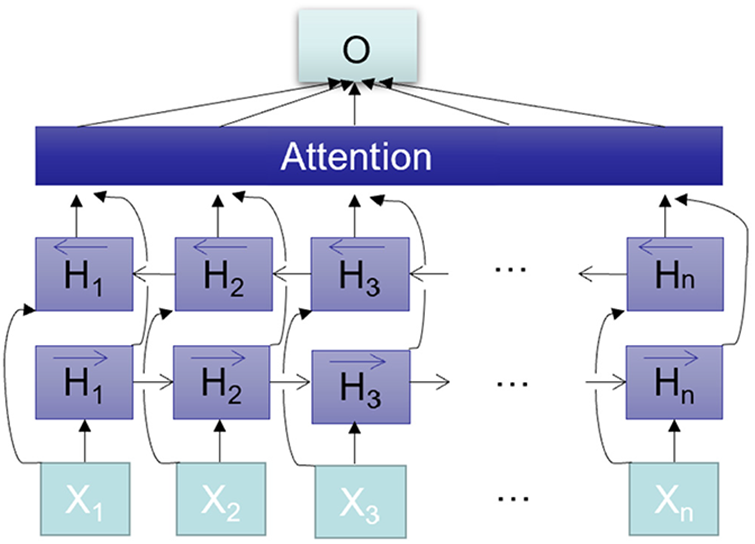
Figure 6: Model structure chart

5  Model Training

5.1 Experimental Configuration

The hardware host for the experiments uses AMD Ryzen5 4600H equipped with NVIDIA GTX2060ti and 16G RAM; the software uses pytorch3.7.8 and the environment of keras2.3.1 and tensorflow1.15.2 [3].

5.2 Evaluation Indicators

The total number of samples in this experiment is 16992, including 2016 prediction samples, and the ratio of the training set to test set is 7:1. In most of the articles, only the traffic flow of weekdays is predicted, and the traffic flow prediction of non-working days is omitted. By observing the original data, it can be obtained that the traffic flow on non-working days is different from the traffic flow on working days due to the interference of various external factors. In contrast, the traffic flow of a whole week is predicted in this paper, and the accuracy of the model prediction is not reduced, and a better result is achieved. In the test set of traffic flow prediction, two main evaluation indexes are set: Root Mean Square Error (RMSE) and Mean Absolute Error (MAE), which is calculated by Eqs. (21) and (22).

RMSE=1n∑i=1n(qi−q^i)2(21)

MAE=1n∑i=1n|qi−q^i|(22)

5.3 Model Training

The model’s input is the historical traffic data and eight essential parameters, such as flow, occupancy, speed, etc. The output is the traffic forecast data of the last seven days, and then the model’s accuracy is measured by comparing the traffic data of the last seven days in the dataset.

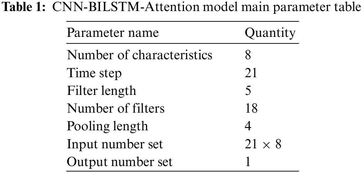
When using PyTorch to reproduce the results, due to the random nature of the algorithm, the same data and code run twice sometimes have very different results, so it is necessary to set a random seed, which can reduce the variability of the model reproduction. This experiment uses the Adam optimizer for parameter optimization. The Adam optimizer can update the variables using the historical information of the gradient with a learning rate of 0.001 and 300 iterations, and its main parameters are set in Table 1.

5.4 Performance Assessment

To check the model’s accuracy, this experiment compared the prediction results of the benchmark models BiLSTM and CNN-BiLSTM with the prediction results after adding Kalman filtering. It was found that the training results of the data without Kalman filtering were poor in both models, but the prediction accuracy of both models was significantly improved after the data were processed by Kalman filtering, and the specific results are shown in Fig. 7.

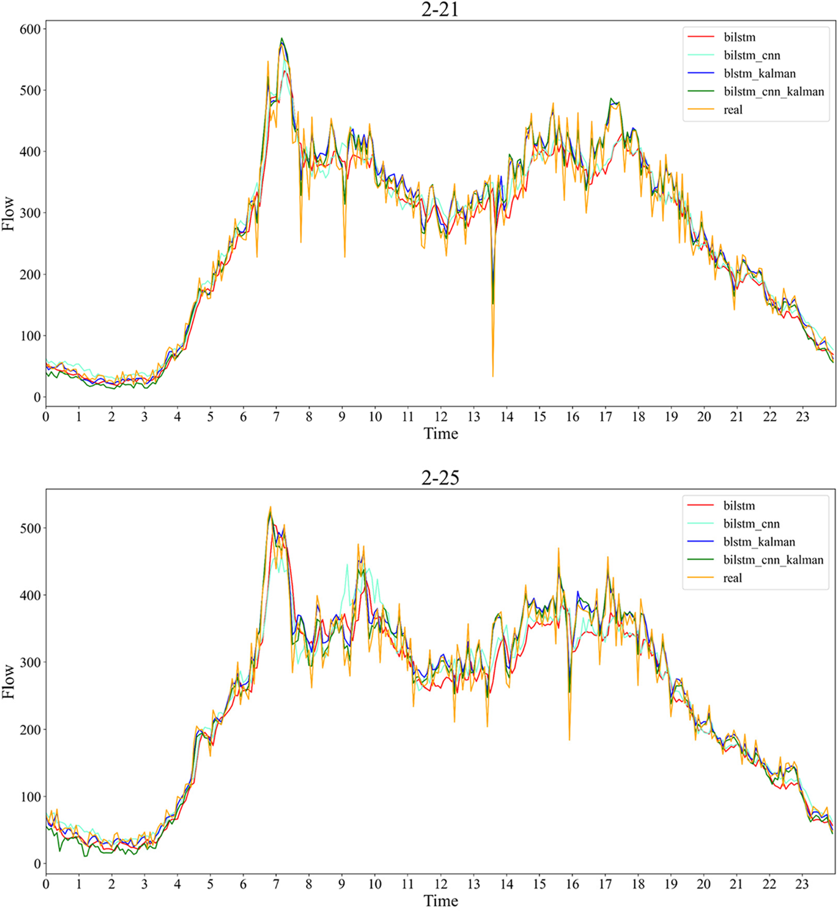
Figure 7: Comparison of the prediction results of the four models on 2.21 and 2.25

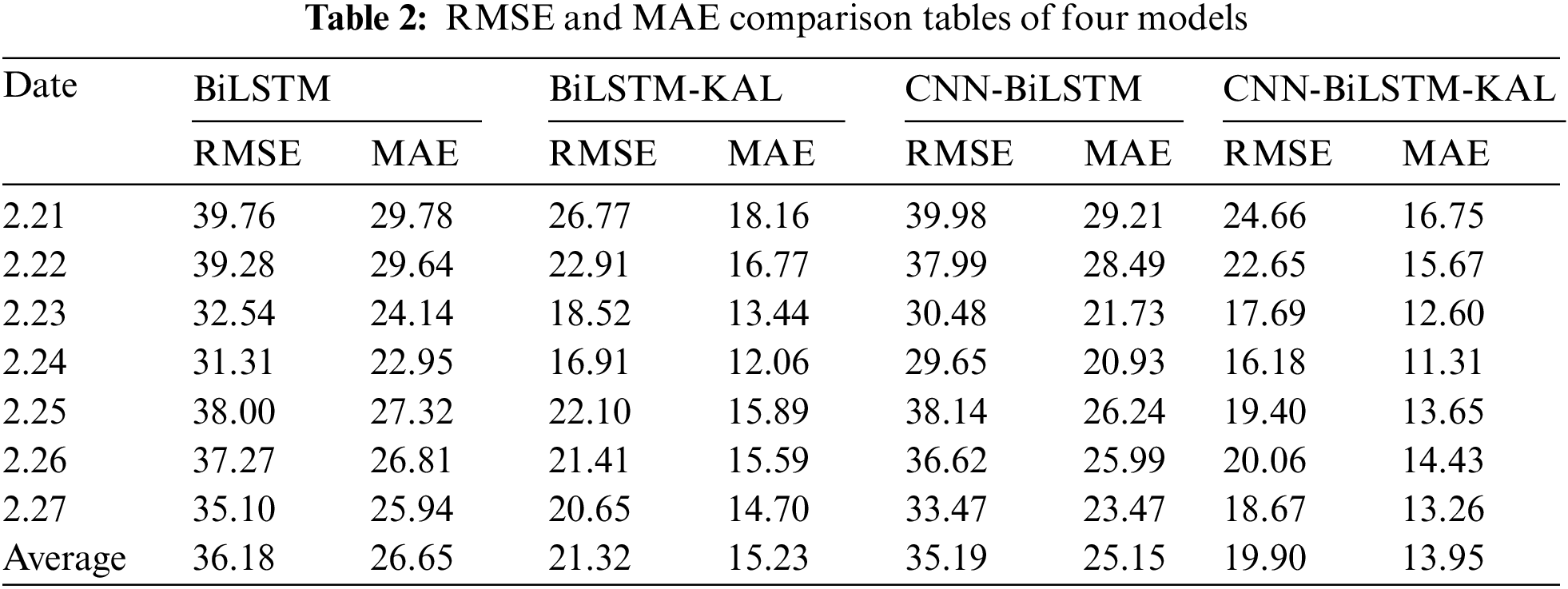
The experimental results show that the experimental results of both the BiLSTM model and the CNN-BiLSTM model with the addition of Kalman filtering fit better. By comparing the loss functions RMSE and MAE of the four models, it was found that in the seven-day prediction set, the RMSE and MAE values of both the BiLSTM-Kal model and the CNN-BiLSTM-Kal model were significantly smaller than BiLSTM and CNN-BiLSTM models. The resultant data are tallied in Table 2. The RMSE of the BiLSTM-Kal model is 21.32, which is a reduction of 14.86 compared to the BiLSTM model, and the MAE is 15.23, which is a reduction of 11.42 compared to the BiLSTM model; The RMSE of the CNN-BiLSTM-Kal model is 19.90, which is a reduction of 15.29 compared to the CNN-BiLSTM model, and the MAE is 13.95, which is a reduction of 11.2 compared to the CNN-BiLSTM model.

To continue to improve the experimental results, this experiment added the Attention Mechanism to the CNN-BiLSTM-Kal model to improve the experimental accuracy by assigning feature weights. The above experimental results are for the traffic flow prediction of seven days a week, because the traffic flow on weekends is complex and unstable, considering that adding the weekend traffic prediction work may reduce the accuracy of the model, so in most of the experimental results given in the article, the weekend traffic prediction work is omitted, but many families will choose to travel and play on weekends. To consider the safety of travel, we need to know the traffic flow at each time point on weekends. Therefore, this experiment compared the prediction results of weekday traffic only with the prediction results of the whole week (February 24th and 25th are non-working days). The results obtained are shown in Fig. 8.

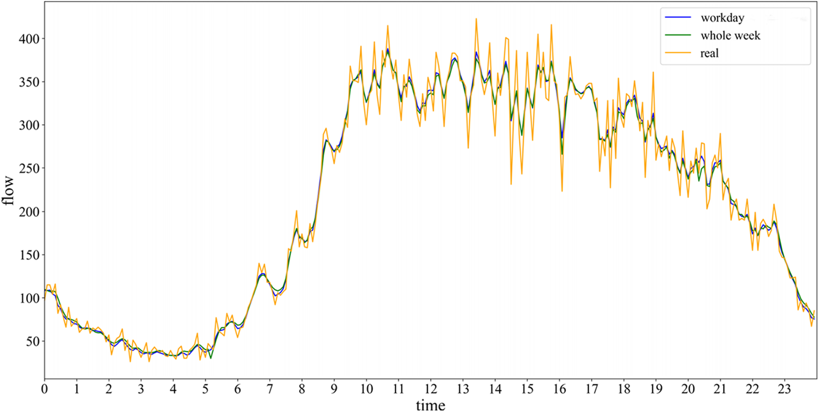
Figure 8: The prediction graph after adding the Attention Mechanism

The experimental results show that the prediction results fit better after adding the Attention Mechanism, and the RMSE of the Kal-CNN-BiLSTM-Attention model shrinks by 2.29 and the MAE shrinks by 1.18 compared to the CNN-BiLSTM-Kal model in the prediction results of whole weekday traffic, as shown in Table 3. Compared with the average result of predicting traffic flow only on weekdays, the MAE of the whole week prediction result is reduced by 0.01, and only the RMSE is increased by 0.58, which is caused by the irregularity of weekend traffic flow.

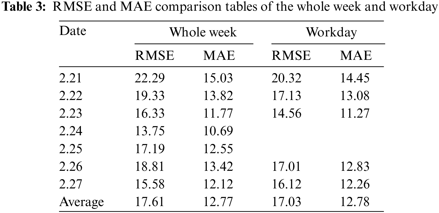
Fig. 9 shows the prediction performance of the Kal-CNN-BiLSTM-Attention model is compared with other commonly used models:

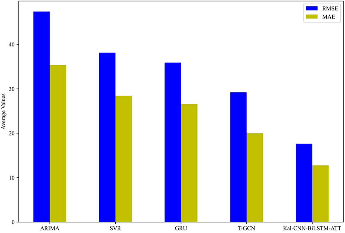
Figure 9: Comparison of prediction results of different methods

(1)   ARIMA: It is a well-known time series analysis method for predicting future values.

(2)   SVR: The mapping relationship between input and output is obtained by training, and then the prediction is performed.

(3)   Gate Recurrent Unit (GRU): It uses gate recurrent unit training data for short-term traffic flow forecasting.

(4)   Temporal Graph Convolutional Network (T-GCN): This model captures both spatial and temporal dependencies by using a combination of GCN and GRU, and finally performs short-term traffic flow forecasting.

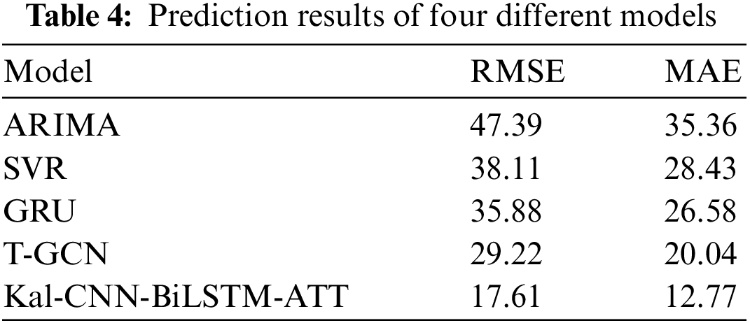
The experimental results show that the prediction results of the CNN-BiLSTM-Attention model based on Kalman-filtered data processing are better than other models. Table 4 shows the specific prediction results of the four different models.

To verify the model’s applicability, the experiment was re-run by replacing two sets of traffic flow data, which were obtained from different detectors. The experimental results are shown in Fig. 10.

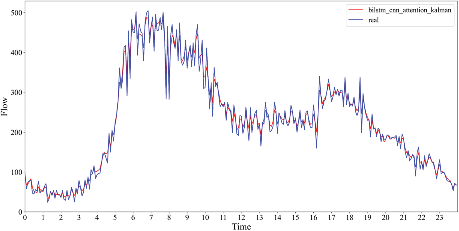
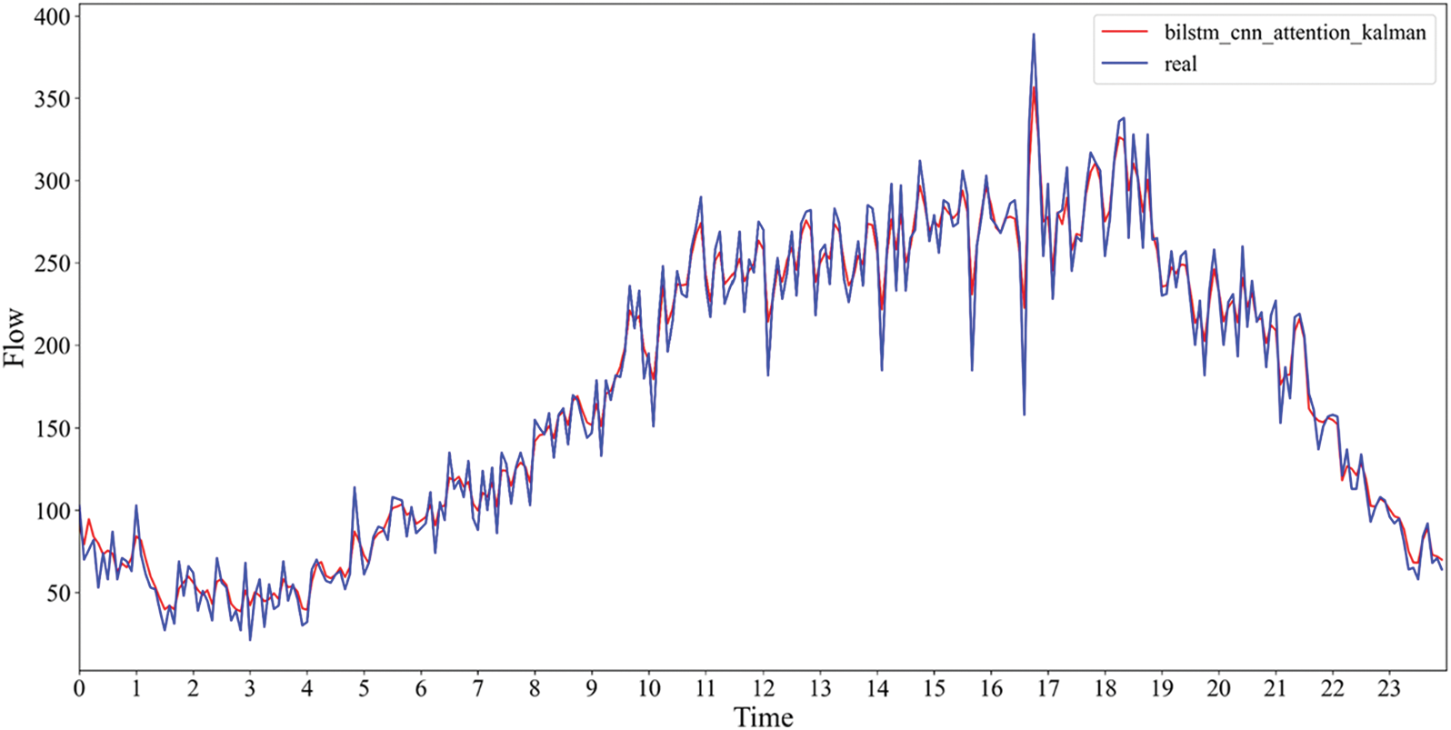
Figure 10: Prediction results of the fifth and tenth detectors

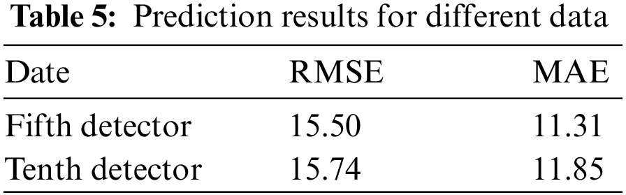
Fig. 10 depicts the better fit of the prediction results for these two data sets. Their RMSE and MAE are smaller than the above experiments. The experimental results show that the model can cope with different data and has high stability. The specific prediction results are tallied in Table 5.

6  Conclusion

This experiment first used the Kalman filter to smooth out the original fluctuating data, which reduces the universality of data due to external interference and applies to a broader range of data. Then the one-dimensional CNN was combined with BiLSTM to comprehensively analyze the three features and sequence information of flow, occupancy, and speed. Finally, the Attention Mechanism was added to the CNN-BiLSTM benchmark model to reduce the loss function by assigning feature weights, thus improving the experimental results. Compared with the CNN-BiLSTM model alone, the Kal-CNN-BiLSTM-Attention model has reduced RMSE by 17.58 and MAE by 12.38.

In this paper, multiple traffic flow prediction methods are effectively combined. By using Kalman filter to process the data, it not only improves the prediction accuracy, but also makes the model applicable to a broader range of data. This model can be applied to traffic flow forecasting in a variety of conditions, including weekends and holidays. At the same time, there are some shortcomings in this experiment, such as not considering external factors, such as rain, snow, traffic accidents, and highway rerouting; these factors can cause deviations in the simulation results of the prediction model. When making traffic flow prediction, not only the local geographical correlation but also the global regional relationship needs to be considered. Multi-scale self-attentive networks can be used to obtain the instantaneous dynamics at different time resolutions in future research. All of these are the focus of future research in traffic flow prediction.

Funding Statement: This research is supported by the Supported by Program for Young Talents of Science and Technology in Universities of Inner Mongolia Autonomous Region (No. NJYT23060).

Conflicts of Interest: The authors declare that they have no conflicts of interest to report regarding the present study.

References

1. H. Lei and S. H. Yi, “Short-term traffic flow prediction of road network based on deep learning,” IET Intelligent Transport Systems, vol. 14, no. 6, pp. 495–503, 2020. [Google Scholar]

2. A. Emami, M. Sarvi and S. A. Bagloee, “Using Kalman filter algorithm for short-term traffic flow prediction in a connected vehicle environment,” Journal of Modern Transportation, vol. 27, no. 3, pp. 222–232, 2019. [Google Scholar]

3. Q. Z. Hou, J. Q. Leng, G. S. Ma, W. Y. Liu and Y. X. Cheng, “An adaptive hybrid model for short-term urban traffic flow prediction,” Physic A: Statistical Mechanics and its Applications, vol. 527, pp. 121065, 2019. [Google Scholar]

4. P. Sun, N. Aljeri and A. Boukerche, “Machine learning-based models for real-time traffic flow prediction in vehicular networks,” IEEE Network, vol. 34, no. 3, pp. 178–185, 2020. [Google Scholar]

5. L. Zhao, Y. J. Song, C. Zhang, Y. Liu, P. Wang et al., “T-GCN: A temporal graph convolutional network for traffic prediction,” IEEE Transportations on Intelligent Transportation Systems, vol. 21, no. 9, pp. 3848–3858, 2020. [Google Scholar]

6. J. J. Tang, J. Zeng, Y. W. Wang, H. Yuan, F. Liu et al., “Traffic flow prediction on urban road network based on license plate recognition data: Combining attention-LSTM with genetic algorithm,” Transportmetrica A: Transport Science, vol. 17, no. 4, pp. 1217–1243, 2021. [Google Scholar]

7. N. A. M. Razali, N. Shamsaimon, K. K. Ishak, S. Ramli, M. F. M. Amran et al., “Gap, techniques and evaluation: Traffic flow prediction using machine learning and deep learning,” Journal of Big Data, vol. 8, no. 1, pp. 1–25, 2021. [Google Scholar]

8. N. Li, L. Hu, Z. L. Deng, T. Su and J. W. Liu, “Research on GRU neural network satellite traffic prediction based on transfer learning,” Wireless Personal Communications, vol. 118, no. 1, pp. 815–827, 2021. [Google Scholar]

9. X. Chen, S. Zhang and L. Li, “Multi-model ensemble for short-term traffic flow prediction under normal and abnormal conditions,” IET Intelligent Transport Systems, vol. 13, no. 2, pp. 260–268, 2019. [Google Scholar]

10. X. J. Zhang and Q. R. Zhang, “Short-term traffic flow prediction based on LSTM-XGBoost combination model,” Computer Modeling in Engineering & Sciences, vol. 125, no. 1, pp. 95–109, 2020. [Google Scholar]

11. A. Miglani and N. Kumar, “Deep learning models for traffic flow prediction in autonomous vehicles: A review, solutions, and challenges,” Vehicular Communications, vol. 20, no. C, pp. 100184, 2019. [Google Scholar]

12. W. B. Zhang, Y. H. Yu, Y. Qi, F. Shu and Y. H. Wang, “Short-term traffic flow prediction based on spatiotemporal analysis and CNN deep learning,” Transportmetrica A: Transport Science, vol. 15, no. 2, pp. 1688–1711, 2019. [Google Scholar]

13. M. Alduhayyim, A. A. Albraikan, F. N. Aiwesan, H. M. Burbur, M. Alamgeer et al., “Modeling of artificial intelligence based traffic flow prediction with weather conditions,” Computers, Materials & Continua, vol. 71, no. 2, pp. 3953–3968, 2022. [Google Scholar]

14. L. Z. Zhang, N. R. Alharbe, G. C. Luo, Z. Y. Yao, Y. Li et al., “A hybrid forecasting framework based on support vector regression with a modified genetic algorithm and a random forest for traffic flow prediction,” Tsinghua Science and Technology, vol. 23, no. 4, pp. 479–492, 2018. [Google Scholar]

15. M. W. Shuai and H. X. Tian, “Long short-term memory based on differential evolution in passenger flow forecasting,” Journal of Simulation, vol. 7, no. 1, pp. 17–21, 2019. [Google Scholar]

16. X. X. Feng, X. Y. Ling, H. F. Zheng, Z. H. Chen and Y. W. Xu, “Adaptive multi-kernel SVM with spatial-temporal correlation for short-term traffic flow prediction,” IEEE Transactions on Intelligent Transportation Systems, vol. 20, no. 6, pp. 2001–2013, 2019. [Google Scholar]

17. X. L. Luo, D. Y. Li and S. R. Zhang, “Traffic flow prediction during the holidays based on DFT and SVR,” Journal of Sensors, vol. 2019, no. 10, pp. 1–10, 2019. [Google Scholar]

18. T. Ma, C. Antoniou and T. Toledo, “Hybrid machine learning algorithm and statistical time series model for network-wide traffic forecast,” Transportation Research Part C: Emerging Technologies, vol. 111, pp. 352–372, 2020. [Google Scholar]

19. S. Fukuda, H. Uchida, H. Fujii and T. Yamada, “Short-term prediction of traffic flow under incident conditions using graph convolutional RNN and traffic simulation,” IET Intelligent Transport Systems, vol. 14, no. 8, pp. 936–946, 2020. [Google Scholar]

20. D. Impedovo, V. Dentamaro, G. Pirlo and L. Sarcinella, “TrafficWave: Generative deep learning architecture for vehicular traffic flow prediction,” Applied Sciences, vol. 9, no. 24, pp. 1–14, 2019. [Google Scholar]

21. F. Kong, J. Li, B. Jiang and H. B. Song, “Short-term traffic flow prediction in smart multimedia system for internet of vehicles based on deep belief network,” Future Generation Computer Systems-the International Journal of EScience, vol. 93, no. 8, pp. 460–472, 2019. [Google Scholar]

22. W. H. Chen, J. Y. An, R. F. Li, L. Fu, G. Q. Xie et al., “A novel fuzzy Deep-learning approach to traffic flow prediction with uncertain spatial-temporal data features,” Future Generation Computer Systems-the International Journal of EScience, vol. 89, no. 8, pp. 78–88, 2018. [Google Scholar]

23. Y. L. Xiao and Y. Yin, “Hybrid LSTM neural network for short-term traffic flow prediction,” Information, vol. 10, no. 3, pp. 105, 2019. [Google Scholar]

24. W. W. Jiang and J. Y. Luo, “Graph neural network for traffic forecasting: A survey,” Expert Systems with Applications, vol. 207, no. 7, pp. 117921, 2022. [Google Scholar]

25. J. X. Ye, J. J. Zhao, K. J. Ye and C. Z. Xu, “How to build a graph-based deep learning architecture in traffic domain: A survey,” IEEE Transactions on Intelligent Transportation Systems, vol. 23, no. 5, pp. 3904–3924, 2020. [Google Scholar]

26. H. H. Dong, Z. Y. Meng, Y. M. Wang, L. M. Jia and Y. Qin, “Multi-step spatial-temporal fusion network for traffic flow forecasting,” in 2021 IEEE Intelligent Transportation Systems Conf. (ITSC), Indianapolis, USA, pp. 3412–3419, 2021. [Google Scholar]

27. D. W. Seng, F. S. Lu, Z. Y. Liang, X. Y. Shi and Q. M. Fang, “Forecasting traffic flows in irregular regions with multi-graph convolutional network and gated recurrent unit,” Frontiers of Information Technology & Electronic Engineering, vol. 22, no. 9, pp. 1179–1193, 2021. [Google Scholar]

28. D. Wang, C. C. Wang, J. H. Xiao, Z. Xiao, W. W. Chen et al., “Bayesian optimization of support vector machine for regression prediction of short-term traffic flow,” Intelligent Data Analysis, vol. 23, no. 2, pp. 481–497, 2019. [Google Scholar]

29. Y. Lv, Y. Duan, W. Kang, Z. Li and F. Y. Wang, “Traffic flow prediction with big data: A deep leaning approach,” IEEE Transactions on Intelligent Transaction Systems, vol. 16, no. 2, pp. 865–873, 2015. [Google Scholar]

30. Y. F. Chen, M. Guizani, Y. Zhang, L. Wang, N. Grespi et al., “When traffic flow prediction and wireless big data analytics meet,” IEEE Network, vol. 33, no. 3, pp. 161–167, 2019. [Google Scholar]

31. M. Ishaq Mustaqeem and S. Kwon, “A CNN—assisted deep echo state network using multiple time-scale dynamic learning reservoirs for generating short-term solar energy forecasting,” Sustainable Energy Technologies and Assessments, vol. 52, no. part c, pp. 102275, 2022. [Google Scholar]

32. Mustaqeem and S. Kwon, “CLSTM: Deep feature-based speech emotion recognition using the hierarchical ConvLSTM network,” Mathematics, vol. 8, no. 12, pp. 2133, 2020. [Google Scholar]