Context Awareness by Noise-Pattern Analysis of a Smart Factory

1  Introduction

Deep learning techniques find patterns in data, and then classify and predict new data; this minimizes the need for repeated human interventions and yields objective results [1]. The first step in deep learning is data preprocessing; raw data are converted into vector or tensor information [(xi,yi) pairs] for training, where x is a multidimensional vector composed of several features and y is the class for that vector. The use of raw data is problematic; the data may be inconsistent and noisy, and the class distributions may be uneven; also, it is difficult to derive effective training data using simple data conversion techniques. To improve training accuracy, data cleaning is employed to resolve discrepancies and noise, and labeling is used to enter the y-values of training data. In other words, there is a need to refine the data or add related data [2]. Processing irregular data prior to deep learning ensures that all distribution patterns are well-represented, and that the data are of good quality. This is essential to increase the performance and reliability of deep learning, but is very time-consuming.

Deep-learning techniques are applied in various industrial fields, including sound processing, to diagnose faults and identify defects by detecting abnormal vibrational and noise signals (e.g., equipment used in smart factories). However, most studies used techniques such as the Mel Frequency Cepstral Coefficient (MFCC) or Mel spectrogram to extract sound-specific features, and then employed the resulting spectral images as training data for convolutional neural networks (CNNs). Conversion of raw data into image data is very time-consuming, and modeling is much slower than when raw data serve as the training data.

Therefore, in this paper, numerical raw material data was used to reduce the time cost required to construct a dataset, and a two-step data preprocessing process was proposed to build it into an efficient training dataset. The model was then designed and learned by inputting the built dataset, and the results were compared and analyzed using two datasets with different data types as input data for the learning model for performance comparison. The data was collected by considering that the frequency pattern activated by the operating sound is different depending on the condition of the fan in the machine, which is an important component of industrial facilities. Operation of these fans is essential for maintaining a productive working environment and is typically operated continuously for long durations, and improper assembly or maintenance can result in malfunctions, including vibrations and audible noise [3]. Sudden fan shutdown can cause serious failure, and fan failure leads to conditions that reduce worker productivity and product quality [4]. Therefore, It is important to detect fan malfunctions early, effectively, and accurately. After collecting the data, we built a training dataset for fan noise pattern analysis using two-step data preprocessing. The first step involved analysis of the sound signals and extracted features, and a Floor-with-Average (FwA) algorithm was used in the second step to prevent overfitting; the dataset becomes too large when all extracted data are used as training data. By filtering the data, the time required to build a training dataset was reduced compared to previous studies. The time from data collection to model evaluation was analyzed using a numerical dataset constructed after two-step data-preprocessing and a graphical image dataset. Training accuracy differed only slightly between the two types of model input, but building a training dataset using image data was much more time-consuming than when using numerical data.

The detection of anomalies has become very important due to huge industrial development and advancements. The detection of anomalies can help identify the reason for the anomaly and detect machine failure, therefore helping to fix it and prevent further damages, which will reduce costs, waste, and improve the efficiency of the machines and increase productivity with lower costs [5]. In addition, as real-time detection is required for anomaly detection, it is expected that the state can be detected at a faster rate than in previous studies if classification is conducted based on numerical data by applying the algorithm proposed in this paper. In addition, sound monitoring in a smart factory is expected to be cost-effective as it has the advantage of relatively inexpensive and easily deployable hardware.

The remainder of the paper is organized as follows. In Section 2, we review prior studies classified by applying deep-learning technology to data converted from sound signals emitted by machines into spectral images for automating existing machine fault diagnosis and anomaly detection. Section 3 describes how we preprocess sound data collected for inputting into deep-learning models using the Fast Fourier Transform (FFT) technique. Section 4 describes the overall system structure and techniques used, including the FwA algorithm and data augmentation technique. Section 4 describes the overall system structure and techniques used, including the FwA algorithm and data augmentation technique. In Section 5, we train a model using a training dataset built as described in the previous section and discuss the results. Section 6 summarizes the work and provides conclusions.

2  Related Works

Smart factories are key in the manufacturing process in the era of the 4th industrial revolution and can be defined as a manufacturing system with multiple devices connected to a centralized cloud-based system and two-way information exchange between the Internet and the cloud [6]. The focus of the smart factory is to create new value using data, but it can also solve conventional problems. One example is the anomaly detection of malfunctioning machines on a production line, a critical operation in manufacturing. This avoids serious damage to machines and products, and economic losses, and in the past, this detection was carried out manually by the Phenomenon Inspection Service [7]. However, not only is it difficult for humans to perform all inspections, but some abnormalities in the production process can threaten the safety of people using industrial machines in factories, so using technology to detect and prevent them before they become dangerous is required [8]. Therefore, research to achieve anomaly detection automation by using artificial intelligence to train large amounts of data to identify events different from standard patterns in the dataset is drawing attention.

1The following Table 1 summarizes the contents of a previous study classified by applying deep-learning technology to data converted from a sound signal emitted by a machine into a spectral image for automating machine fault diagnosis and anomaly detection [9–15].

Table 1 shows that most studies classified sounds using graphical images derived by applying various feature extraction techniques to raw sound data. However, although the time required to build the raw dataset was short, the time needed to build the image dataset (by converting raw data into images) was long. Also, many studies did not compare the total dataset construction time, instead focusing on accuracy alone. We subjected numerical raw data to two-step preprocessing to build efficient training datasets, and compared model performance between the numerical and image datasets.

3  Background–Sound Data Preprocessing

Sounds are analog data generated via vibration. Sound recognition is a form of pattern recognition involving sound signal preprocessing, feature extraction, and the establishment of a training model and classification modules (Fig. 1) [16].

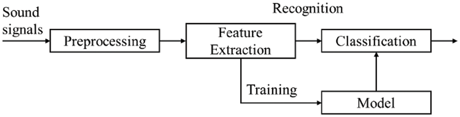
Figure 1: Sound data preprocessing

Sound signals that are digitally converted via sampling and quantization are high dimensional. Also, as a signal may exhibit several frequencies, it is difficult to extract features by applying deep learning to raw sounds. Therefore, the feature extraction process that generates the data in a form that the model can learn well is important, and through this, the most relevant information is obtained from the original sound signal data and the sound feature vector of the signal is formed [17]. The types of feature extraction techniques include The Fourier Transform (FT), Fast Fourier Transform (FFT), Short-time Fourier Transform (STFP), and Mel Frequency Cepstral Coefficient (MFCC). In this paper, we construct a training dataset to extract and classify features of recorded fan sound data by applying the FFT technique, one of the most common conversion techniques that perform DFT fast among several techniques and provide information on all frequency components of soundsignals [18].

4  System Design

This section discusses our system architecture and the methods used for data collection, preprocessing, and augmentation. The system development process for determining machine abnormality and type based on operation noise data by fan state was developed by experimental design, experimental setup, data collection, data preprocessing, data augmentation, model development, and model evaluation, as shown in Fig. 2.

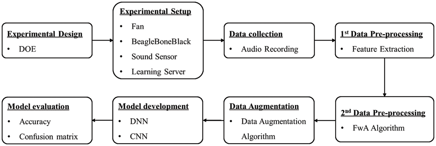
Figure 2: Development procedure of the proposed context awareness system

4.1 System Architecture

In this paper, we propose a system architecture as shown in Fig. 3. The proposed system consists of two modules, which show the role and progress of each module.

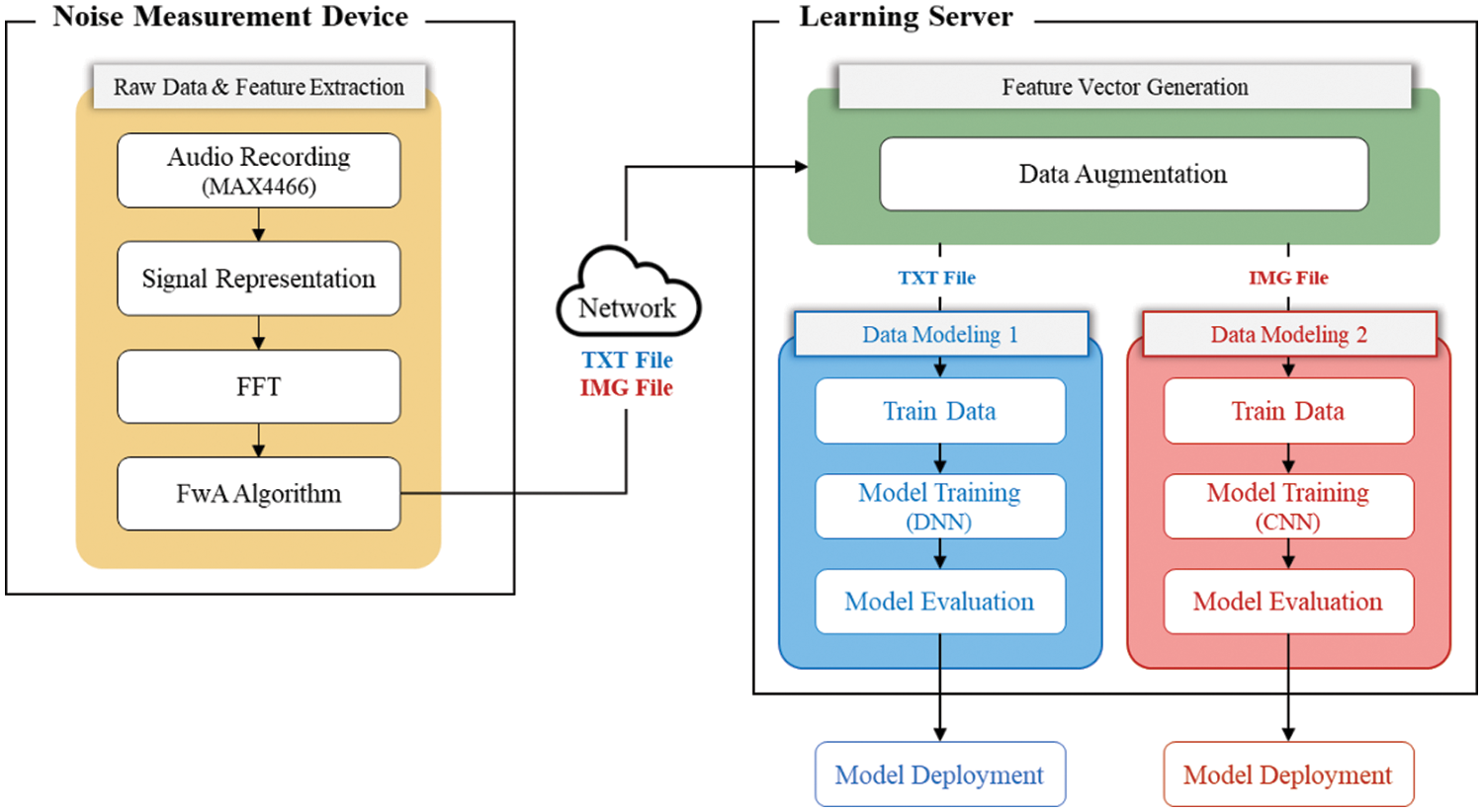
Figure 3: System architecture

First, in the noise-measurement device located on the left side of Fig. 3, fan noise is collected through the sound sensor, and two stages of data preprocessing are carried out. The initial process consists of analyzing sound-signal information and extracting features by applying FFT techniques, and the second is the process of preventing overfitting by filtering data through the FwA algorithm (in Section 4.3) proposed in this paper.

Next, in the Learning Server, the numerical data was first extracted through the noise-measuring device, and the image data was converted into a graph divided and the data-augmentation technique was applied to build the training dataset. Afterwards, to classify the fan status using the built-up training dataset, the numerical dataset is input to the designed Deep Neural Network (DNN) model, and the image dataset is input to the CNN model to proceed with training, evaluate the performance, and deploy the most suitable model.

The training dataset was divided into numerical and image data, and the time from data preprocessing to model deployment was compared between the two data types. Section 5 describes the experimental process proposed in this paper in detail through each module of the system architecture shown in Fig. 3.

4.2 Fan Noise Data Collection

To identify differences in frequency according to fan state, the frequency band was set to 0~7,500 Hz. The fan was connected to a Direct Current (DC) motor, power (6 V) was supplied and noise was recorded. Abnormal, normal, and pinch were collected and classified into three states, and the status of the fan in which the abnormal and normal states were collected can be checked through Fig. 4. Pinched data were collected using wooden chopsticks to simulate a foreign object caught in the fan.

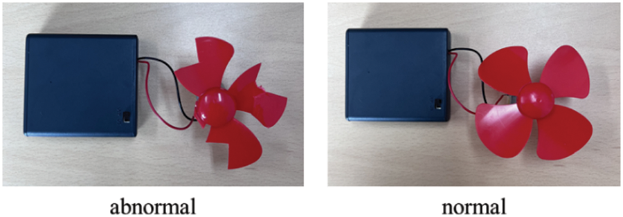
Figure 4: Fan status classifications

4.3 Data Preprocessing

The collected noise data are combinations of several different frequencies and are thus fairly large, which makes it difficult to extract features using a deep-learning model. Therefore, the data preprocessing that generates the data in a form that the model can read well and a form that the model can train well is important. In the method proposed in this paper, it is preprocessed through two steps.

The first preprocessing step consists of applying the FFT technique of the frequency domain among the methods of converting the digital signal to extract the features of the fan noise data. The sampling rate was 1.5 MHz (in line with the specifications of the noise-measuring device; see Section 5 [System Implementation and Results] for details). In the 0~7,500 Hz band, FFT is applied to 65,536 values per file. If these are used as a training dataset without additional preprocessing, overfitting occurs because the data volume is excessive. A second preprocessing step is required; therefore, we developed and tested a FwA algorithm. The pseudo-code is shown in Fig. 5; the algorithm filters the data to build a training dataset based on meaningful information. The data are filtered by rounding down the decimal point of the frequency data and averaging the amplitude data mapped to the corresponding frequency band. Fig. 9 shows that the 65,536 values were reduced to 7,500 in this manner.

Figure 5: The FwA algorithm

The FwA algorithm is applied after the FFT step in Fig. 3 (where i refers to frequency data and j to amplitude data by frequency). At this time, the two types of data are mapped one-to-one in the form of [Hz: amplitude] (lines 01~03). First, the decimal point is removed by applying a rounding down operation to the Hz data of the same band among the recorded data (lines 04~07). Create a variable to find amplitude data corresponding to the same frequency band (lines 08~09). If amplitude data corresponding to Hz data in the same band is listed, data are inserted into the declared variable, otherwise, the number of amplitude data previously contained is counted and averaged by dividing it by the sum of amplitude data. Through this process, the final dataset is constructed by filtering the data (lines 10~22).

To build an efficient training dataset as described above, two-step preprocessing was applied; the results are shown in Section 5.3.

4.4 Data Augmentation

Currently, we are relying on data-driven deep-learning approaches to achieve high performance in the area of sound-signal processing. However, the high performance achieved is highly dependent on the quantity and quality of the data. Depending on the specific task, such data can often be hard to obtain and costly to label particularly in the audio domain. A solution to this problem is posed by data augmentation, a process that artificially creates new input data from existing samples that are altered in a way that they differ from the original sample while still maintaining the information that is relevant for the respective task at hand [19].

Data augmentation is a technology that increases the amount of data through various algorithms based on a small amount of the original dataset. Insufficient data is a high risk of underfitting and overfitting in addition to not reflecting the characteristics of the dataset well when training the model [20]. We generated additional data by multiplying the amplitudes by a random value between 0.9000 and 1.0999, and adding the result to the original values. The results are shown in Section 5.4.

5  System Implementation and Results

5.1 Experiment Environment

In this paper, we implement a noise measurement device using BeagleBoneBlack (BBB), a single-board small computer that provides low price and low energy consumption. BBB provides sufficient computational power for various types of IoT applications, such as Raspberry Pi and Arduino, while also having digital and analog I/O and on-board persistent storage devices. Table 2 lists the BBB specifications [21,22].

Fig. 6 shows the system experimental architecture. We connected a MAX4466 sound sensor to the BBB (Table 2) to collect noise data for each fan state; a device of the type shown in Fig. 4 was used to collect noise data three times in each state. As we used time and accuracy as performance indicators, the data were divided into numerical (txt) and image (img) data. This was followed by two-step preprocessing, and the results were transmitted to the learning server via the network.

Figure 6: System experimental architecture

The training server was an NVIDIA Quadro RTX 5000 GPU (Ubuntu Server 20.04.2 LTS operating system). Numerical and image data-based training algorithms were implemented using the Keras (ver. 2.7.0) and TensorFlow (ver. 2.8.0) machine learning libraries, respectively. The preprocessed data received from the noise-measuring device were augmented to construct the final training dataset, and the training model was built to fit the final numerical and image datasets.

5.2 Fan Noise Data Collection Results

As shown in Section 4.2, the fan status was divided into three categories: abnormal, normal, and pinch, and recorded 3 times for each status. There are a total of 9 types of data, and the FFT technique is applied to the measured data according to the system architecture in Fig. 3 and saved as a txt extension file and an img extension file, respectively. The Noise Measuring Device consists of two CPU cores. One is an ARM core mainly used in embedded systems and the other is a Programmable Real-time Unit (PRU) core that is efficient for real-time processing. This PRU core had the capability to process commands with a maximum clock of 200 MHz [23]. However, since the language used in this study was written in high-level Python, many cycles were used to process commands, allowing data to be sampled at a rate of up to 1.5 MHz. In addition, to solve the Aliasing problem that occurs during noise collection, the sampling rate was set to a frequency band that used only 7,500 Hz, which is 1/2 of 1.5 MHz, for research. Therefore, as shown in Fig. 7, it can be confirmed that the change in amplitude according to the set frequency (Hz) band 0~7,500 Hz is expressed in a graph. Using this data as training data requires a complex deep-learning model with a large amount of data, and at the same time, the number of parameters increases, which takes a lot of training time, and furthermore, there are disadvantages that training is not performed properly because the performance of the training server is not supported. To solve this shortcoming, in this paper, the FwA algorithm shown in Fig. 5 was proposed and applied, and the applied result is shown in Fig. 8.

Figure 7: FFT Results according to fan state

Figure 8: FwA algorithm result: IMG file

5.3 Data Preprocessing Results

We built an efficient training dataset; the final results (after two-step preprocessing) for the image and text files are shown in Figs. 8 and 9, respectively. The FwA algorithm only changes the amplitudes in the fixed frequency band. The amount of training dataset should be augmented because deep-learning training performance deteriorates because these data are not sufficient to be used as a training dataset. However, it is not easy to secure sufficient training datasets due to time and cost. Therefore, one of the methods used to train a model, even with an insufficient dataset, is data augmentation. In this paper, the final training dataset was constructed by applying data augmentation based on the conditions as shown in Section 4.4.

Figure 9: FwA algorithm result: TXT file

5.4 Training Dataset

As a result of three experiments for each fan state, data-augmentation techniques were applied to the data and augmented by 200 pieces, and the corresponding data were combined to generate 600 pieces of data per fan state. Therefore, the total data for the total three fan states is 1,800, and since the sampled data per file has a size of 7,500, the shape of the input data (x_data) becomes (1,800, 7,500). When an input value is given, a label (y_data) for the input value must be given to proceed with the training. Therefore, labels were assigned with values of 0, 1, and 2 for abnormal, normal, and pinch states, respectively, and have shapes (1,800, 1) the same as input data. Image data also consists of 600 pieces of data per fan state, a total of 1,800 pieces. In general, according to studies that it is good to set the ratio of the training dataset and the validation dataset to about 8:2, the dataset was configured in the corresponding ratio and trained.

5.5 Numerical Data-Based Learning Model Structure

Our numerical data-based training model is a classification model employing a DNN with eight layers (including the input and output layers). The number of nodes in the input layer was determined to be the same as the size of the input vector. The output layer uses softmax [24] activation to distinguish between the abnormal, normal, and pinched states (depending on the input data). All input data were vectors of the amplitudes at each frequency band (≤15 kHz). There were six hidden layers with 100, 512, 128, 100, 64, and 24 nodes. The input of a node in the current layer is determined by the output of a node in the previous layer. Input attributes are obtained from noise data by fan state, and the input of the node becomes an input parameter of the activation function, and the result of the activation function is passed to the next layer and used for node input at the next layer. For state inference, the ReLU [25] activation function, which is a non-linear activation function for each layer, is used. In this paper, since the fan state must be divided into three categories as previously defined, softmax is used as the activation function of the output node. The number of nodes was set to three equals the number of categories. To measure the loss between the actual and predicted outputs, we used sparse_categorical_crossentropy, which is utilized in multiple classification problems. After repeating training and evaluation, hyperparameters such as epoch and batch size were adjusted, the final structure of the model was determined, and dropout 0.2 was applied to each layer to prevent overfitting. Fig. 10 shows the model based on numerical data.

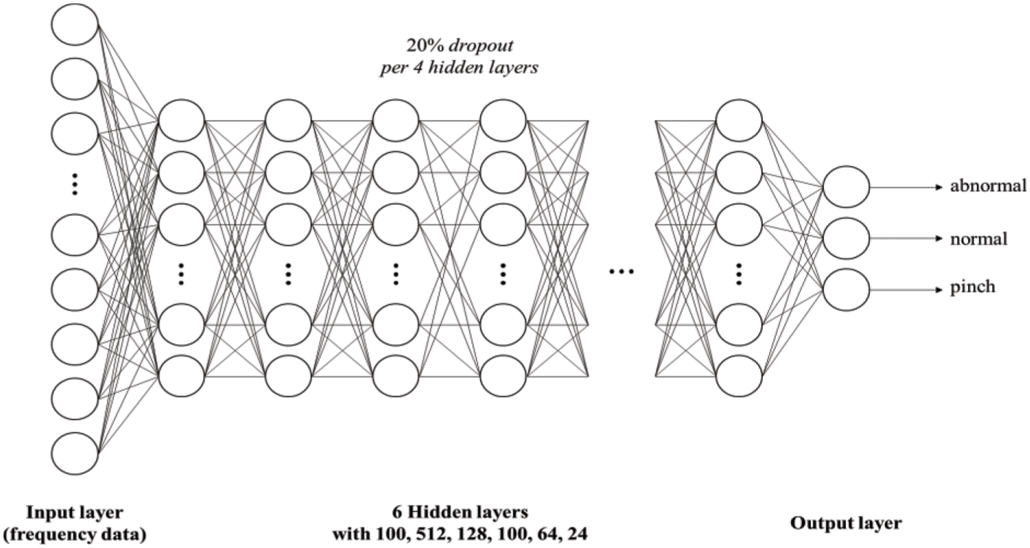
Figure 10: Deep neural network used to infer fan state

5.6 Image Data-Based Learning Model Structure

The image data–based learning model was a CNN model. The image data-based learning model used a CNN model. CNN is a type of feed-forward artificial neural network that can extract features from images and classify images using convolution operations, or detect objects (i.e., car, tree, man, dog) in images through features [26]. In addition, research on classifying sound using CNN is also being actively conducted. In this paper, as shown in Fig. 11, it consists of a total of 3 Convolution layers, 1 Flatten layer, and 4 Dense layers. Each Convolutional layer consists of 64 nodes consisting of a 3 × 3 convolutional filter, and ReLU is used as the activation function. For all Convolutional layers, a dropout of 20% to reduce overfitting and 2 × 2 max-pooling to reduce the size of feature maps were performed together. One Flatten layer serves to convert a two-dimensional feature map to one dimension, which is entered as a Dense layer. A Dense layer allows more efficient learning because only the reduced-dimensional Feature Map is input and connected to the output [27]. Except for the last Dense layer, the activation functions of the rest of the dense layers use ReLU, which is fast to learn and has a small amount of computation. The activation function of the last Dense layer uses softmax to configure the output as many as the number of classes to be classified. Adam (Adaptive Moment Estimation), a combination of Momentum and Root Mean Square Propagation (RMSProp), was used as the Optimizer, an optimization algorithm [28–31]. The total number of weights and biases in the model was 2,321,283.

Figure 11: Convolution neural network used to infer fan state

5.7 Training Results

Fig. 12 shows the training accuracies and losses when numerical and image data were used. During training, 1,800 data were employed (see Section 5.4). For the model structure, the numerical data has the same structure as Section 5.5, and the image data has the same structure as Section 5.6. To evaluate the performance of the model, 80% was divided into training data and 20% was divided into test data. In this paper, the performance is based on the time taken to distribute the training model, so the model training parameters of epoch 50 and batch size 64 are applied equally to both models. Trainset_acc and Trainset_loss are values that evaluate the performance of the model with the data used for training, and Testset_acc and Testset_loss are values that evaluate the performance of the model with new data not used for training. The training results showed that training was satisfactory; accuracy was high and loss was minimal. The training and test results did not differ significantly and there was no overfitting.

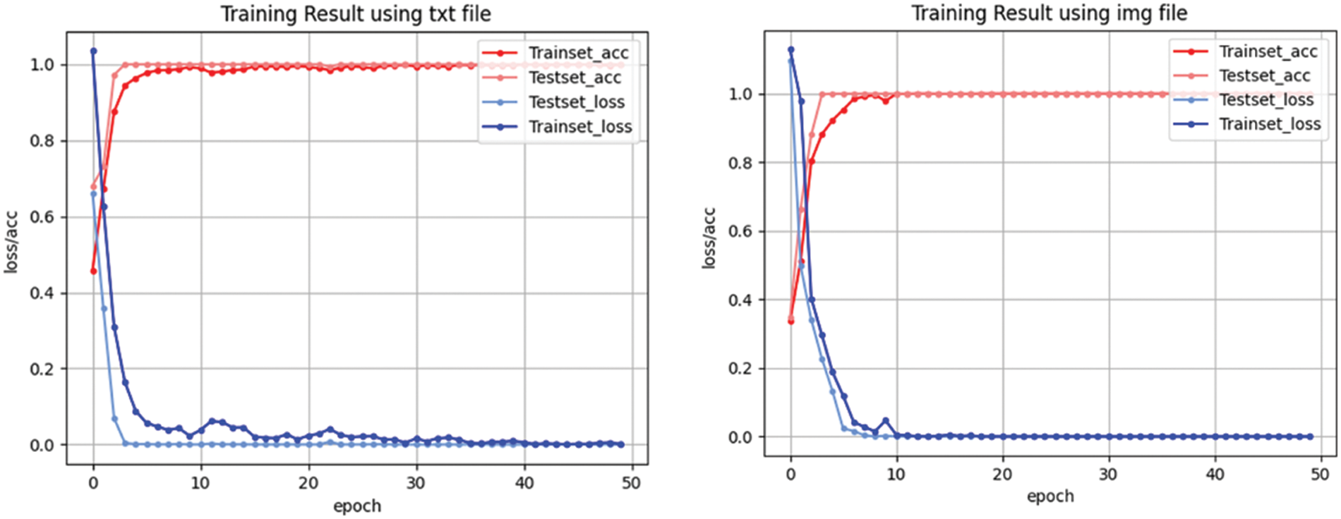
Figure 12: Training accuracy and loss graphs

We analyzed the learning results by deriving performance indicators for each class from the training and test data. We calculated a confusion matrix for the test data and checked all classification results. In ML or DL, the Confusion Matrix is a standard tool that visualizes how accurate a trained model can predict from a respective validation dataset [32]. Fig. 13 shows the training results (as a Confusion Matrix) based on the image data for all three classes. The rows are the actual class labels and the columns the predicted labels. As a result of the analysis, it can be confirmed that the predicted value and the actual value for each class coincide with a high probability because a mechanical sound with a small frequency change is input as data.

Figure 13: The CNN confusion matrix

5.8 Comparison of Time Spent in the Entire Experimental Process

To compare the performance of our method to that of previous ones, the data were separated into numerical values (txt) and images (img), and then used for learning. Fig. 14 is a graph showing the total time required for the experiment, from the process of collecting and preprocessing data, the process of augmenting the preprocessed data, and the process of evaluating the model through the training dataset. The x-axis means the progressed step, the y-axis means the time is taken, and the unit is seconds (sec). When the experiment was conducted using text file data with numerical data listed, it took 16 s in the preprocessing, 23 s to augment it into a training dataset, and 22 s until evaluation through the designed model after building the training dataset, which took a total of 61 s. In comparison, when an experiment was conducted using image data converted from numerical data into a graph, 20 s in the preprocessing, 183 s to augment it into a training dataset, and 24 s until evaluation through the designed model after building the training dataset, took a total of 227 s. Comparing the time required, we can confirm that it took about nine times longer than it took to augment the numerical data in the process of augmenting the data to build the image data as a training dataset. In this way, it should be seen that detection based on numerical data (txt) applied with the FwA algorithm, an algorithm proposed in this paper, acts as an important factor in detecting states at a faster rate compared to existing studies based on image learning. In addition, in this paper, we experimented with only 1,800 training datasets, but in deep-learning, the higher the training performance is as a training dataset is used with large amounts of good quality data. Therefore, the time required for the data augmentation process, which is a process for constructing numerical data and image data as a training dataset, was additionally compared, and the result is shown in Fig. 15. The x-axis means the number of constructed training datasets, the y-axis means the time taken, and the unit is seconds (sec). In this way, applying the algorithm proposed in this paper to a system for detecting the abnormal sound of a fan in a machine, it can be confirmed that the use of numerical raw data as a training dataset is faster than the previous study of the use of image data as a training dataset.

Figure 14: Experimental time comparison graph

Figure 15: Time spent on data augmentation graph

6  Conclusion

We developed a two-step data preprocessing method to reduce the time required to build a training dataset for image data-based detection of abnormal sounds. A system for determining machine abnormality and type based on operating sound data by fan status in the machine was implemented, and the time required for each data was compared and analyzed. First, fan noise is collected, and data preprocessing is performed in two steps. The data preprocessing method consists of applying the FFT technique to analyze the collected noise signal information and extracting features and filtering the data by applying the FwA algorithm to prevent overfitting. Next, a training dataset was constructed by applying the data-augmentation technique, and the numerical dataset was input as the input data of the DNN model, and the image dataset was input as the input data of the CNN model to proceed with learning and evaluating the performance. It can be seen that the two-stage data preprocessing process reduces the time required to build a learning dataset, and it can also be seen that it takes about 5.2 times more time to build a dataset using image data compared to numerical data.

Recently, deep-learning models have been widely used in machine defect detection and diagnosis systems, and with the continuous rapid development of computer technology, Massachusetts Institute of Technology (MIT) neuroscientists have developed an Artificial Intelligence (AI) model that can estimate the location of objects with a sound like humans through AI [33]. Applying this technology to a factory with many machines would be expected to effectively detect machine defects. Therefore, we will collect more data considering various state parameters in the future. In addition, we will continue to conduct research based on the achievement of smart factories in the future by strengthening the stability and robustness of the system in consideration of sounds that exist complexly in the actual environment.

Acknowledgement: None.

Funding Statement: This work was supported by the National Research Foundation of Korea (NRF) grant funded by the Korea Government (MSIT) (No. 2021R1C1C1013133), this work was funded by BK21 FOUR (Fostering Outstanding Universities for Research) (No. 5199990914048), and this work was supported by the Soonchunhyang University Research Fund.

Author Contributions: Conceptualization, Lee and Kim; methodology, Lee and Kim; software, Lee and Park; validation, Lee and Park; formal analysis, Lee and Kim; investigation, Lee; resources, Lee; writing––original draft preparation, Lee; writing––review and editing, Kim; All authors have read and agreed to the published version of the manuscript.

Availability of Data and Materials: The data used in this paper can be requested from the corresponding author upon request.

Conflicts of Interest: The authors declare that they have no conflicts of interest to report regarding the present study.

1Acc = Accuracy, Pre = Precision, Rec = Recall, CNN = Convolutional Neural Network, DBN = Deep Belief Network, SVM = Support Vector Machine, GRU = Grated Recurrent Unit.

References

1. H. S. Kim, J. H. Chung and W. K. Baek, “A study on a motor noise diagnosis method using voice recognition and machine learning techniques,” Transactions of the Korean Society for Noise and Vibration Engineering, vol. 31, no. 1, pp. 40–46, 2021. [Google Scholar]

2. E. H. Kim, K. H. Lee and W. K. Sung, “Recent trends in lightweight technology for deep neural networks,” Communications of KIISE, vol. 38, no. 8, pp. 18–29, 2020. [Google Scholar]

3. C. A. Gong, H. Lee, Y. Chuang, T. Li, C. S. Su et al., “Design and implementation of acoustic sensing system for online early fault detection in industrial fans,” Journal of Sensors, vol. 2018, no. 5, pp. 1–15, 2018. [Google Scholar]

4. D. K. Chaturvedi and D. Singh, “Development of Intelligent test bench for ceiling fan,” in 2013 5th Int. Conf. on Computational Intelligence and Communication Networks, Mathura, India, pp. 574–579, 2013. [Google Scholar]

5. Y. A. Ahmed, H. Othman and M. A. M. Salem, “Comparative study of different activation functions for anomalous sound detection,” in 2021 Int. Conf. on Microelectronics, New Cairo City, Egypt, pp. 207–211, 2021. [Google Scholar]

6. H. Wu, Y. Shen, X. Xiao, A. Hecker and F. H. P. Fitzek, “In-Network processing acoustic data for anomaly detection in smart factory,” in 2021 IEEE Global Communications Conf., Madrid, Spain, pp. 1–6, 2021. [Google Scholar]

7. S. Hatanaka and H. Nishi, “Efficient GAN-based unsupervised anomaly sound detection for refrigeration units,” in 2021 IEEE 30th Int. Symp. on Industrial Electronics, Kyoto, Japan, pp. 1–7, 2021. [Google Scholar]

8. B. Bayram, T. B. Duman and G. Ince, “Real time detection of acoustic anomalies in industrial processes using sequential autoencoders,” Expert Systems, vol. 38, no. 1, pp. e12564, 2021. [Google Scholar]

9. O. Janssens, V. Slavkovikj, B. Vervisch, K. Stockman, M. Loccufier et al., “Convolutional neural network based fault detection for rotating machinery,” Journal of Sound and Vibration, vol. 377, no. 6, pp. 331–345, 2016. [Google Scholar]

10. L. Wen, X. Li, L. Gao and Y. Zhang, “A new convolutional neural network-based data-driven fault diagnosis method,” IEEE Transactions on Industrial Electronics, vol. 65, no. 7, pp. 5990–5998, 2018. [Google Scholar]

11. C. Lee, J. Jwo, H. Hsieh and C. Lin, “An intelligent system for grinding wheel condition monitoring based on machining sound and deep learning,” IEEE Access, vol. 8, pp. 58279–58289, 2020. [Google Scholar]

12. T. Tran and J. Lundgren, “Drill fault diagnosis based on the Scalogram and Mel Spectrogram of sound signals using artificial intelligence,” IEEE Access, vol. 8, pp. 203655–203666, 2020. [Google Scholar]

13. K. W. Kang and K. M. Lee, “CNN-based automatic machine fault diagnosis method using spectrogram images,” Journal of the Institute of Convergence Signal Processing, vol. 21, no. 3, pp. 121–126, 2020. [Google Scholar]

14. W. Zhu, H. Liu, Y. Zhou, L. Gan and Y. Ma, “Wind turbine blade fault detection by acoustic analysis: Preliminary results,” in 2021 IEEE Int. Conf. on Signal Processing, Communications and Computing, Xi’an, China, pp. 1–5, 2021. [Google Scholar]

15. T. Tran, N. T. Pham and J. Lundgren, “A deep learning approach for detection drill bit failures from a small sound dataset,” Scientific Reports, vol. 12, no. 1, pp. 1–13, 2022. [Google Scholar]

16. C. Honggang, X. Mingyue, F. Chenzhao, S. Renjie and L. Zhe, “Mechanical fault diagnosis of GIS based on MFCCs of sound signals,” in 2020 5th Asia Conf. on Power and Electrical Engineering, Chengdu, China, pp. 1487–1491, 2020. [Google Scholar]

17. Y. He, I. Ahmad, L. Shi and K. H. Chang, “SVM-based drone sound recognition using the combination of HLA and WPT techniques in practical noisy environment,” KSII Transactions on Internet and Information Systems, vol. 13, no. 10, pp. 5078–5094, 2019. [Google Scholar]

18. G. Allwood, X. Du, K. M. Webberley, A. Osseiran and B. J. Marshall, “Advances in acoustic signal processing techniques for enhanced bowel sound analysis,” IEEE Reviews in Biomedical Engineering, vol. 12, pp. 240–253, 2019. [Google Scholar] [PubMed]

19. S. Mertes, A. Baird, D. Schiller, B. W. Schuller and E. André, “An evolutionary-based generative approach for audio data augmentation,” in 2020 IEEE 22nd Int. Workshop on Multimedia Signal Processing, Tanpere, Finland, pp. 1–6, 2020. [Google Scholar]

20. H. C. Cho and J. S. Moon, “A layered-wise data augmenting algorithm for small sampling data,” Journal of Internet Computing and Services, vol. 20, no. 6, pp. 65–72, 2019. [Google Scholar]

21. J. Patoliya, S. B. Patel, M. Desai and K. Patel, “Embedded linux based smart secure IoT intruder alarm system implemented on BeagleBone Black,” Soft Computing and its Engineering Applications, vol. 1374, pp. 343–355, 2020. [Google Scholar]

22. D. G. Costa and C. Duran-Faundez, “Open-source electronics platforms as enabling technologies for smart cities: Recent developments and perspectives,” Electronics, vol. 7, no. 12, pp. 404, 2018. [Google Scholar]

23. G. Cloey, “Beaglebone black system reference manual,” Texas Instruments Dallas, vol. 5, pp. 108, 2013. [Google Scholar]

24. S. Sharma, S. Sharma and A. Athaiya, “Activation functions in neural networks,” International Journal of Engineering Applied Sciences and Technology, vol. 4, no. 12, pp. 310–316, 2020. [Google Scholar]

25. V. Spoorthy, M. Mulimani and S. G. Koolagudi, “Acoustic scene classification using deep learning architectures,” in 2021 6th Int. Conf. for Convergence in Technology, Maharashtra, India, pp. 1–6, 2021. [Google Scholar]

26. J. Lee, D. Jang and K. Yoon, “Automatic melody extraction algorithm using a convolutional neural network,” KSII Transactions on Internet and Information Systems, vol. 11, no. 12, pp. 6038–6053, 2017. [Google Scholar]

27. P. Dileep, D. Das and P. K. Bora, “Dense layer dropout based CNN architecture for automatic modulation classification,” in 2020 National Conf. on Communications, Kharagpur, India, pp. 1–5, 2020. [Google Scholar]

28. I. Sutskever, J. Martens, G. Dahl and G. Hinton, “On the importance of initialization and momentum in deep learning,” Proceedings of the 30th Int. Conf. on Machine Learning, Atlanta GA, USA, vol. 28, no. 3, pp. 1139–1147, 2013. [Google Scholar]

29. R. V. Kumar Reddy, B. Srinivasa Rao and K. P. Raju, “Handwritten Hindi digits recognition using convolutional neural network with RMSprop optimization,” in 2018 Second Int. Conf. on Intelligent Computing and Control Systems, Madurai, India, pp. 45–51, 2018. [Google Scholar]

30. R. Zaheer and H. Shaziya, “A study of the optimization algorithms in deep learning,” in 2019 Third Int. Conf. on Inventive Systems and Control, Coimbatore, India, pp. 536–539, 2019. [Google Scholar]

31. D. P. Kingma and J. Ba, “Adam: A method for stochastic optimization,” in Int. Conf. on Learning Representations, San Diego, USA, 2015. [Google Scholar]

32. F. J. P. Montalbo and A. S. Alon, “Empirical analysis of a fine-tuned deep convolutional model in classifying and detecting malaria parasites from blood smears,” KSII Transactions on Internet and Information Systems, vol. 15, no. 1, pp. 147–165, 2021. [Google Scholar]

33. A. Francl and J. H. McDermott, “Deep neural network models of sound localization reveal how perception is adapted to real-world environments,” Nature Human Behaviour, vol. 6, no. 1, pp. 111–133, 2022. [Google Scholar] [PubMed]