Research on Optimization of Dual-Resource Batch Scheduling in Flexible Job Shop

1  Introduction

With the rapid development and application of automated production workshops and intelligent manufacturing models, automated production has been realized gradually in traditional flexible workshops. In the actual production process of flexible automated production workshops, in addition to some large or special product parts, the processing and transfer process of most parts is carried out according to a certain batch, and the task of workpiece transfer is mainly undertaken by AGV, so the quality of a batch division of workpieces and the transfer efficiency of AGV will have a huge impact on the production efficiency of workshops [1]. For the traditional flexible job shop scheduling problem (FJSP), only machine and process constraints were considered, and only machine allocation and process sequencing were needed to optimize without involving workpiece batching, workpiece transfer time, and AGV paths planning, which can no longer meet the actual production needs [2]. Therefore, based on traditional FJSP, the dual-resource batch scheduling in the flexible job shop studied in this paper comprehensively considers workpiece batching and workpiece transfer time and integrates the two resources of machine and AGV for scheduling, which has important theoretical significance and practical application value.

Scholars have carried out a lot of research on the dual resource scheduling problem of the flexible job shop. He et al. [3] considered the huge impact of AGV and machine resource scheduling on the production cycle, established a dual-resource scheduling mathematical model, and used a hybrid genetic algorithm to solve it. To solve the FJSP problem of integrated AGV, Xu et al. [4] proposed a cooperative hybrid evolutionary algorithm, which is more competitive than other algorithms in solving the FJSP problem with AGV. Li et al. [5] established an integrated optimization model of the flexible job shop machine and AGV designed the whale optimization algorithm and verified the feasibility of the optimization scheme through test cases. Aiming at the flexible job shop scheduling problem of segmented AGV, Liu et al. [6] established a dual-resource scheduling mathematical model of machine tool and AGV with the minimum completion time as the optimization objective, designed an improved genetic algorithm to solve it, and then verified the superiority of the algorithm through a standard case. Chen et al. [7] established a mathematical optimization model for the automated flexible workshop scheduling problem with AGV as the main means of transportation and improved the efficiency of problem-solving by improving the discrete particle swarm algorithm. By solving the cases on the benchmark data set, it was found that the efficiency improvement of the production system by the number of AGVs conformed to the law of diminishing marginal effects. When Paksi et al. [8] analyzed the workshop production process, they believed that the task configuration of the two production resources, the machine, and the worker, would affect the processing cycle. They solved the problem by using an improved genetic algorithm and achieved better results. Scholars such as Li et al. [9] believed that workers in flexible workshops, as flexible production resources like machines, would have a huge impact on the production environment, so they proposed a water wave optimization decision-making method with the lowest total energy consumption as the optimization goal, which was verified by a large number of simulation experiments. Zhang et al. [10] considered the different loading and unloading times of workers due to individual factors and improved the quantum genetic algorithm through strategies such as niche, adaptive rotation angle, and quantum mutation, which improved the computational efficiency of the algorithm.

Although there are some achievements in the dual resource scheduling problem, the huge impact of the batch division of the workpiece on the overall production cycle is ignored. Xu et al. [11] believed that the randomness of batch division resulted in a too large search space of the optimization scheme, so they proposed a tentative strategy to guide the search direction of the batch scheme and then proposed a parallel process for different batches, which effectively improved the production management capability of the workshop. Xu et al. [12] comprehensively considered factors such as workpiece batching, machine failure, and preprocessing time, established a robust model for batch scheduling optimization of multi-objective flexible job shops, and solved the problem through an improved Non-dominated Ranked Genetic Algorithm (NRGA) algorithm. And the superiority of this algorithm was verified by calculation. Liu et al. [13] established a scheduling model and a corresponding disjunctive graph model for the variable batch scheduling and used the improved migratory bird algorithm to solve the model. Tan et al. [14] established an integrated optimization model for batching and scheduling of flexible job shops and used an improved genetic algorithm to numerically solve problems of different scales, proving the superiority of the algorithm, and analyzing the effect of different batching strategies on scheduling results. The research results have certain guiding significance for factories to improve their production management level. Bozek et al. [15] proposed a two-stage optimization algorithm to solve the flexible workshop batch scheduling optimization problem with variable batching and verified the effectiveness of the two-stage optimization algorithm. Huang et al. [16] proposed an improved hybrid ant colony algorithm to solve the multi-objective batch scheduling problem of batch division, batch cost, and completion time. Wu et al. [17] proposed an improved multi-objective optimization algorithm, combined with the idea of reverse scheduling, for the variable batch scheduling problem of the flexible job shop, and finally verified the effectiveness of the algorithm through a set of experiments. Jia et al. [18] proposed a dual-objective ant colony optimization algorithm, in which the user’s preference is incorporated into the solution construction. Numerical experiments show that the algorithm is more excellent at solving large-scale problems. Zeng et al. [19] and other scholars used refined scheduling technology and combined it with the NSGA-II algorithm to solve the dual-resource batch scheduling problem with manufacturing cost and production cycle as optimization goals, and verified the effectiveness of the algorithm through cases.

To sum up, scholars have carried out many studies on the flexible job shop scheduling problem with AGV. The research methods are mainly divided into two categories. One is to assume that the path planning of AGV is known in the scheduling process, without considering the AGV path conflict and collision. Such problems are usually solved by intelligent optimization algorithms. The other is to allocate tasks and plan paths for AGV when the optimal scheduling order of tasks is known. This kind of problem mainly adopts a dynamic programming method. The above two methods do not achieve real dual resource integrated scheduling, because job scheduling and AGV path planning are not completely independent parts, they will affect each other, and it is not realistic to solve them separately. In addition, for the batch scheduling optimization problem of the flexible job shop, most scholars use intelligent optimization algorithms to solve the batch partitioning problem and the sequencing problem of processes on the machine. This problem has become an NP-hard problem, and few scholars can solve the AGV path planning and collision problem together. This is because the flexible job shop dual resource batch scheduling optimization problem has the characteristics of complex constraints, very difficult modeling, and exponentially increasing difficulty in solving problems as the production batch increases. Most scholars have separated the relationship between the batch demand of products in the production process and the dual resource constraints. However, the research on machine and AGV dual resource integrated scheduling considering workpiece batching is more in line with the actual production, and the solution to this complex problem is more universal.

Therefore, according to the coupling relationship and sequence relationship among batch optimization, dual-resource scheduling, and path planning, this paper designs an improved nested optimization algorithm to solve the dual-resource batch scheduling optimization problem of the flexible job shop. The algorithm consists of the outer batch optimization algorithm and the inner dual resource scheduling algorithm. The batch optimization scheme solved by the outer batch optimization algorithm is used as the construction basis of the inner dual-resource scheduling algorithm, and the optimization result of the dual-resource scheduling scheme is also used as the evaluation index of the outer batch optimization algorithm. In addition, the batch optimization scheme and the dual-resource scheduling scheme are used as the decision-making basis for path planning, and the path planning algorithm is also used as the evaluation index of the batch optimization algorithm and the dual-resource scheduling algorithm. Finally, the effectiveness of the algorithm in this paper is verified through the actual case, and the influence of different configurations of AGVs on the scheduling results is analyzed. The specific flow of the improved nested optimization algorithm is shown in Fig. 1.

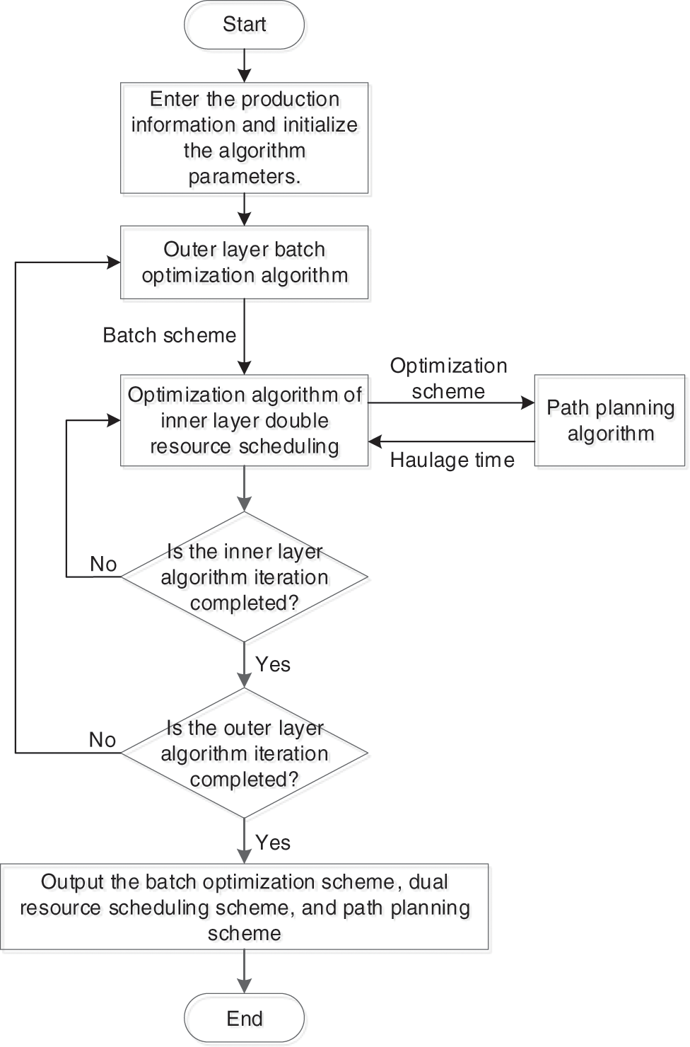
Figure 1: Flow chart of dual-resource batch scheduling optimization in flexible job shop

2  Problem Description and Modeling

The dual-resource batch scheduling problem of the flexible job shop can be described as follows: a flexible workshop has m processing machines, k AGVs and n types of workpieces to be processed, and each type of workpiece Ji has a certain production batch Bi Different machines can be selected for processing, and the processing time will be different depending on the selected processing machine. Each type of workpiece is divided into several sub-batches according to the production batch during processing, and each sub-batch is processed as a whole.

Assumptions:

1.    A single machine can only process one sub-batch at any time. Similarly, a single sub-batch can only be processed by one machine at any time;

2.    The workpiece processed by the machine tool takes a single sub-batch as the processing unit, and cannot be interrupted after starting processing, and the processing time includes the preparation time;

3.    The buffer capacity of each machine tool is infinite, and only one AGV is allowed to be parked at the same time;

4.    There is no process sequence constraint between different sub-batches;

5.    Any batch can only be processed when all batches being processed on the selected machine have been processed;

6.    AGV transfers workpieces in one batch as the transfer unit, and cannot be interrupted after the transfer begins;

7.    The AGV path system is a bidirectional single channel.

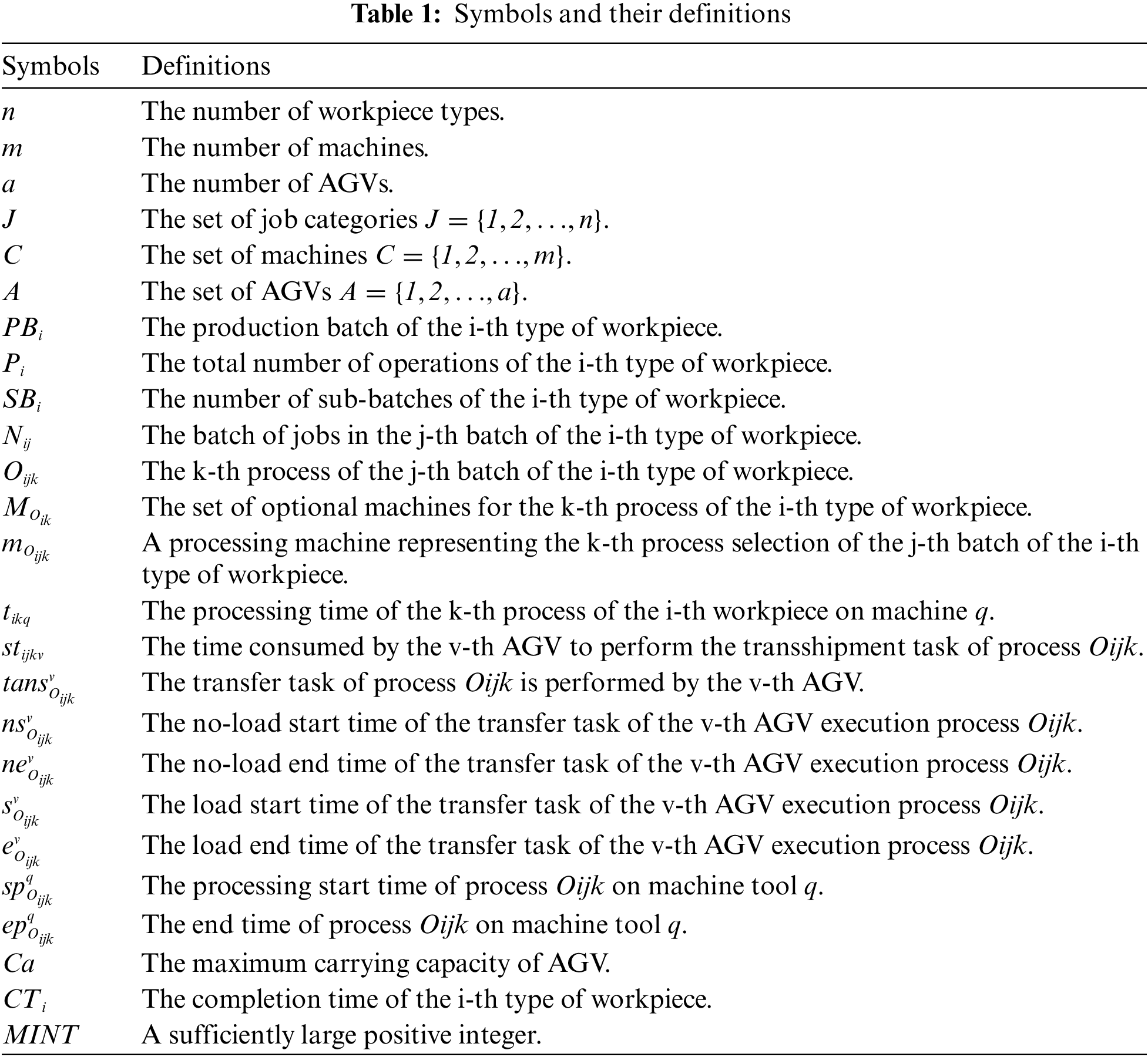
To facilitate the establishment of mathematical models, the symbols introduced are defined in Table 1 according to the above assumptions.

Decision variables:

αijkq={1,Oijkis processed on Cq0,other cases(1)

θijkv={1,Oijkis transported by Av0,other cases(2)

βijkwzxq={1,Oijkis processed on Cq before Owzx0,other cases(3)

γijkwzxv={1,Oijkis transported by Av before Owzx0,other cases(4)

where, i,w∈J={1,2,…,n}; j=SBi; z=SBw; k=Pi; x=Pw; q∈C={1,2,…,m}; v∈A={1,2,…,a}.

Aiming at the optimization of dual-resource batch scheduling in the flexible job shop, the following mathematical model is established with the minimum production cycle as the optimization objective.

Objective function:

f=min{max(CT1,CT2,…,CTn)}(5)

Constraint conditions:

∑j=1SBiNij=PBi(6)

1<Nij<min(Ca,PBi)(7)

spOwzxq+MINT(1−βijkwzxq)≥epOijkq(8)

nsOwzxv+MINT(1−γijkwzxv)≥eOijkv(9)

∑q=1mαijkq=1(10)

∑v=1mβijkv=1(11)

epOijkq=spOijkq+tijq×Nij(12)

eOijkv=sOijkv+stijkv(13)

spOwzxq≥max(epOijkq×(1−βijkwzxq),eOwzxv)(14)

sOijkv≥max(neOijkv,epOi(j−1)kq)(15)

epOi(j−1)kq<spOijkq(16)

mOijk∈MOik(17)

where, i,w∈J={1,2,…,n}; j=SBi; z=SBw; x=Pw; k=Pi; q∈C={1,2,…,m}; v∈A={1,2,…,a}; Eq. (5) is the optimization objective of the mathematical model, namely the minimum production cycle min(Makespan); Eq. (6) indicates that the sum of the batches of each sub-batch of each type of workpiece is equal to the production batch of the workpiece; Eq. (7) stipulates the batch division range of sub-batches; Eq. (8) indicates that the machine tool can only process a batch of workpieces at the same time; Eq. (9) indicates that AGV can only transport a batch of workpieces at the same time; Eq. (10) indicates that a process of each sub-batch can only be processed by one machine tool; Eq. (11) indicates that a process of each sub-batch can only be transported by one AGV; Eq. (12) indicates that the process of a batch of workpieces is not allowed to be interrupted once processing begins; Eq. (13) indicates that the process of a batch of workpieces is not allowed to be interrupted once it begins to be transported; Eq. (14) indicates that the earliest start processing time of the process is the maximum completion time of the current processing process on the machine tool q and the end time of the AGV load; Eq. (15) represents the constraint condition of the load start time of the task; Eq. (16) indicates that each process between each batch of each type of workpiece needs to comply with the process flow; Eq. (17) represents the machining machine selection constraint of the process.

3  Design of Improved Nested Optimization Algorithm

3.1 Design of Outer Layer Batch Optimization Algorithm

The outer batch optimization algorithm is an improved design based on the simulated annealing algorithm (SA), using the improved SA to solve the batch scheme. The concept of the Boltzmann selection function of the genetic algorithm is introduced into the design of the traditional SA acceptance function, which establishes a Boltzmann acceptance function. At the same time, the concept of perturbation operator in variable neighborhood search algorithm is introduced. When the improved SA iterates to a certain threshold m, if the optimal solution has not changed, a new neighborhood solution will be generated by perturbing the current solution, and then the optimal solution is further searched from the neighborhood solution.

The batch of jobs is equally divided, and the batch scheme of each division is expressed in the form of an array {int1,int2,…,intn}. The length of the array is consistent with the number of job types, and the job number corresponds to the subscript of the array one by one. The value in the array represents the number of sub-batches corresponding to the job division, that is, the inti in the array represents the number of specific batches divided by the i-th job according to the equal batching method.

In the search process of the improved SA algorithm, the candidate batch scheme Bcur is generated in each iteration of the algorithm as follows: an element inti is randomly selected in the current batch scheme Bcur, and is replaced by a new number of batch partitions which is randomly selected in the neighborhood set of the element, while other elements in the current batch scheme Bcur remain unchanged. Like the generation of the candidate solution, the perturbation action of the optimal solution randomly selects two elements from the current batch scheme Bcur, and replaces these two elements with a neighborhood solution, with the other elements in the current batch scheme Bcur unchanged. This results in the perturbation action of the current batch scheme.

The solution process of the outer layer batch optimization algorithm is shown in Fig. 2, and the specific steps are as follows:

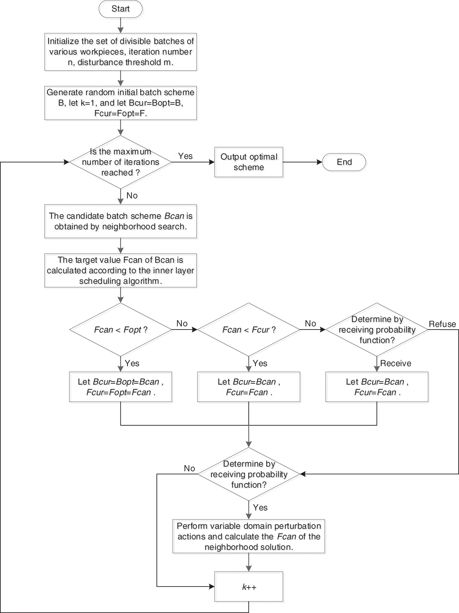
Figure 2: Flow chart of the outer batch optimization algorithm

Step 1: Initialize the iteration number n and the disturbance threshold m of the improved simulated annealing algorithm, and calculate the divisible batch set of various workpieces.

Step 2: Let k=1, the initial batching scheme B is randomly generated according to the divisible batch set of various workpieces, and let Bcur=Bopt=B.

Step 3: Calculate the target value of the initial batching scheme through the inner dual resource scheduling algorithm, and let Fcur=Fopt=F.

Step 4: Determine whether k is equal to the total number of iterations. If k=n, the iteration ends, and the optimal batching scheme and the scheduling scheme under the batching scheme are output. Otherwise, jump to Step 5.

Step 5: The candidate batching scheme Bcan is generated according to Bcur, and the target value Fcan of Bcan is calculated by using the inner dual resource scheduling algorithm.

Step 6: Determine the size of Fcan and Fopt. If Fcan<Fopt, let Bcur=Bcan, Bopt=Bcan, Fcur=Fcan, Fopt=Fcan, and jump to Step 9. Otherwise, jump to Step 7.

Step 7: Determine the size of Fcan and Fcur, if Fcan<Fcur, let Bcur=Bcan, Fcur=Fcan, Bopt remain unchanged, and jump to Step 9; otherwise, jump to Step 8.

Step 8: Generate a random number p between 0 and 1, calculate the receiving probability function Paccp of the candidate batching scheme Bcan, and determine the size relationship between p and Paccp; if p<Paccp, then receive Bcan, let Bcur=Bcan, Fcur=Fcan, and jump to Step 9; otherwise, reject Bcan and jump to Step 9.

Step 9: Determine whether the threshold m is reached. If the disturbance threshold is reached, the variable neighborhood perturbation action is performed on the current solution, and the Fcur of the new current solution is calculated. Otherwise, directly execute Step 10.

Step 10: k++, execute Step 4.

3.2 Design of Inner Dual Resource Scheduling Optimization Algorithm

The inner dual resource scheduling optimization algorithm is an improved design based on an adaptive genetic algorithm. The details are as follows.

3.2.1 Coding

Each chromosome is coded in two layers: Order Select (OS) and Machine Select (MS). Among them, the process layer coding adopts the decimal coding method. The elements of the process layer represent the workpiece number and the workpiece batch, and the order of the same elements represents the order of the process. The machine layer adopts the real number coding method, and each element of the machine layer represents the machine selected according to the total process sequence. Fig. 3 shows a complete coding scheme example.

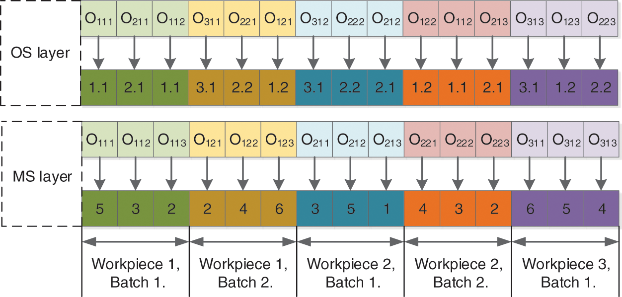
Figure 3: Example of the coding scheme

3.2.2 Decoding

According to the above coding scheme, the activity of the chromosome is decoded, and the AGV is scheduled based on the first-come-first-served rule and the AGV workload balancing rule during the decoding process. The specific decoding steps designed in this paper are as follows:

Step 1: Initialize the processing time record table Mα of each machine, the processing time record table Jt of each process, the driving position record vector Apos of each AGV, the no-load driving time record table AKα of each AGV, the load driving time record table AFα of each AGV, the working time record vector At of each AGV, the idle AGV set Akx, and the time window record table WindowTimepath of each road section;

Step 2: According to the order from left to right, take out the OS layer in the chromosome gene, get the workpiece, batch, and process information, namely Oijk. The completion time of the previous process Oij(k−1) is obtained by comparing it with Jt;

Step 3: Compare the completion time of the immediate process Oij(k−1) with the AKα and AFα of each AGV, and add the AGV with no transportation task after the completion of the immediate process Oij(k−1) to the idle AGV set Akx;

Step 4: Determine if Akx is empty; if Akx is empty, the AGV with the shortest AGV cumulative working time is selected from all AGV sets A for transportation tasks; otherwise, select the AGV with the shortest cumulative working hours from AKα for the transportation task; clear Akx;

Step 5: Determine whether the k of the process Oijk is equal to 1, that is, whether it is the first process of batch j of workpiece i; if k=1, the starting node knodes of the no-load path of AGV is the node at the current position of AGV recorded in Apos, the target node knodet is the node at the location of the warehouse, the starting node fnodes of the load path is the node at the location of the warehouse, and the target node fnodet is the node at the location of the processing machine q of the process. Otherwise, the starting node knodes of the no-load path of AGV is the node of the current position of the AGV recorded in Apos, the target node knodet is the node of the position of the processing machine of the immediately preceding process Oij(k−1), the starting node fnodes of the load path is the node of the position of the processing machine of the immediately preceding process Oij(k−1), and the target node fnodet is the node of the position of the processing machine q of the process;

Step 6: The no-load start time of AGV is the end time of the last transportation task of AGV. The information of AGV no-load start node, target node, no-load start time and WindowTimepath is taken as the input of the Dijkstra algorithm based on the time window. The no-load driving path and no-load driving time of AGV without collision are calculated. The no-load end time of AGV is the sum of the no-load start time and no-load driving time, and Apos is updated;

Step 7: Comparing the AGV no-load end time with the completion time of the immediate pre-process Oij(k−1), the AGV’s load start time is the larger of the two. The starting node, target node, load start time and WindowTimepath of the AGV load are used as the input of the Dijkstra algorithm based on the time window. The load travel path and load travel time of the collision-free AGV are calculated. The load end time of the AGV is the sum of the load start time and the load travel time. Update Apos;

Step 8: Update At, AKα and AFα to complete a complete transportation task of AGV;

Step 9: Decode the activity of the machine, take out the processing machine q of the gene position corresponding to the MS layer process Oijk in the chromosome, and calculate the processing time tijkq of Oijk according to the single processing time and sub-batch;

Step 10: Determine whether the process Oijk is the first process on machine q; if it is the first process of machine processing, perform Step 11; otherwise, perform Step 12;

Step 11: Process Oijk is the first process of machine q processing, then the process Oijk start processing time is AGV load end time;

Step 12: According to the load end time and processing time of the process, find the idle time period that allows the process to insert the job in the machine q job cycle in Mα. If the idle time period is obtained, Step 13 is performed; otherwise, perform Step 14;

Step 13: Compare the AGV load end time with the start time of the idle time period, the start processing time of the process Oijk is the larger value of the two;

Step 14: Comparing the completion time with the load end time of the current process of the machine tool, the starting processing time of the process Oijk is the larger of the two;

Step 15: According to the start processing time and processing time of the process Oijk, calculate the completion time of the process, and update Mα;

Step 16: Determine whether the process Oijk is the last gene on the chromosome, not the last gene transferred to Step 2; otherwise, the calculation is terminated and the maximum completion time and the decoding result are output.

3.2.3 Initialize the Population

For the OS layer of the chromosome in the initial population, a completely random generation strategy is first used, and then the hill-climbing algorithm is used to further select the OS layer of the initial population. For the MS layer of the chromosome, random selection (RS), local selection (LS), and world selection (WS) are combined to select the processing machine for each process.

3.2.4 Selection, Mutation, and Crossover Operation

For the selection of the population, this paper adopts the binary tournament selection method. Two individuals are randomly selected from the population each time and the fitness value is calculated, and then the individual with the best fitness value is selected to enter the next generation population. Repeat the above operation until the new population size reaches the original population size.

The precedence Operation Crossover (POX) operator and Multi-point crossover (MPX) operator are used for the OS layer and MS layer of chromosome respectively. The crossover process of POX and MPX is shown in Figs. 4 and 5. In the figure, P1 and P2 represent the parent chromosome, and C1 and C2 represent the offspring chromosome.

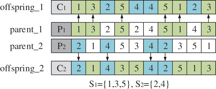
Figure 4: POX crossover process

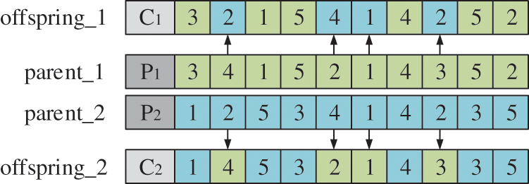
Figure 5: MPX crossover process

The specific steps of POX crossover are as follows:

Step1: The job set is randomly divided into two non-empty subsets S1 and S2;

Step2: Copy the genes contained in S1 in P1 to C1, copy the genes contained in S2 in P2 to C2, and keep their gene positions unchanged;

Step 3: Replicate the genes contained in S1 in P1 to C2, and the genes contained in S2 in P2 to C1, and keep their gene order unchanged.

When performing MPX crossover, multiple crossover points are randomly selected on the parent chromosome, and then the genes on the corresponding crossover points are exchanged.

For the OS layer and MS layer of chromosomes, interchange mutation operation and multipoint mutation operation are used respectively. The interchange mutation operation is shown in Fig. 6, that is, two gene loci are randomly selected from the OS layer of the chromosome for gene exchange. The multi-point mutation operation is shown in Fig. 7, that is, multiple gene loci are randomly selected in the MS layer of the chromosome, and then one other machine tool is randomly selected from the set of optional machine tools on each gene locus to replace the current machine tool.

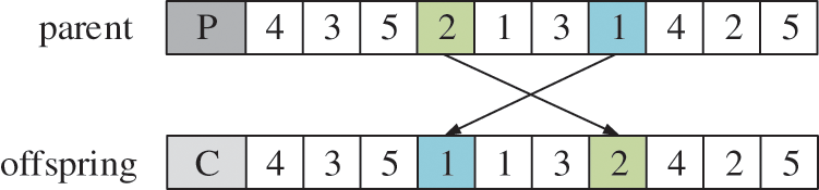
Figure 6: Interchange mutation operation

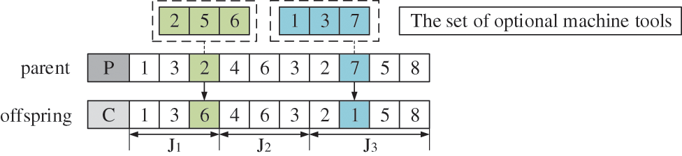
Figure 7: Multi-point mutation operation

3.2.5 Adaptive Crossover and Mutation Probability

Eqs. (18) and (19) are respectively used to solve the adaptive crossover probability and mutation probability:

Pc=k1+(k2−k1)×(1+cos(π×niters)/2(18)

Pm=k3+(k4−k3)×(1+sin(π×niters−π/2))/2(19)

where n represents the number of iterations of the algorithm; iters represents the total number of iterations of the algorithm; k1, k2, k3, k4 represent custom parameters, generally based on experience: k1=k3=0.5, k2=k4=1.

3.3 Design of Path Planning Algorithm

The path planning algorithm in this paper is an improved design of the Dijkstra algorithm based on the time window. The specific contents are as follows:

AGV may have the following conflicts when driving in the workshop: intersection conflict, node occupancy conflict, and opposite conflict. As shown in Figs. 8, 9, and 10.

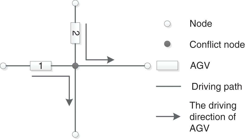
Figure 8: Intersection conflict

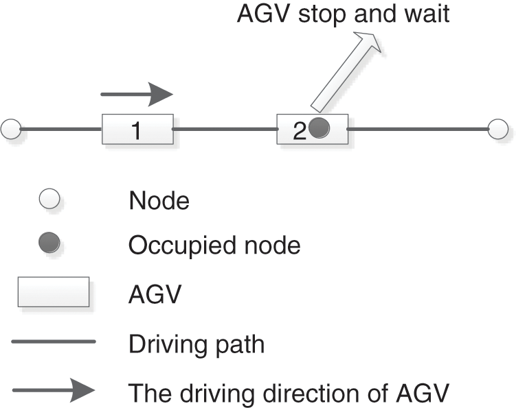
Figure 9: Node occupancy conflict

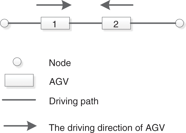
Figure 10: Opposite conflict

For the above three types of conflicts, the conflict resolution strategies adopted are speed control adjustment strategy and re-planning strategy. Determine which strategy to choose, according to Eq. (20). If Eq. (20) is satisfied, choose the speed control and regulation strategy; otherwise, choose the re-planning strategy.

T1+Δt<T2(20)

When there is an extreme situation in the opposite conflict, that is, the re-planning strategy fails. First, all the drivable sections are obtained according to the re-planning strategy, and then the time consumed by each driving section is obtained according to the speed control adjustment strategy. Determine the section selection, according to Eq. (21).

Ti+Δti<Tj+Δtj(21)

where, NewRode is the set of all new road segments generated by the replanning strategy and i,j∈NewRode≠∅; Ti and Tj in Eq. (21) are respectively the travel time of AGVs on road segment i and road segment j, and Δti and Δtj are the time consumed by AGVs respectively on road segment i and road segment j when the speed control regulation strategy is adopted. If Eq. (21) is satisfied, section i is selected, otherwise, section j is selected.

The model for the time window of the road segment can be represented by Eq. (22).

WindowTimei{nodein,nodeout,timein,timeout,AGVid}(22)

where, i∈Road≠∅. WindowTimei denotes the time window of section i, nodein denotes the node number when driving into the section, nodeout denotes the node number when driving out of the section, timein denotes the time node when driving into the section, timeout denotes the time node when driving out of the section, and AGVid denotes the AGV driving on the section during this period. Road represents the set of all sections of the workshop path system.

According to the above time window model and conflict resolution strategy, the conflict resolution process designed in this paper is shown in Fig. 11.

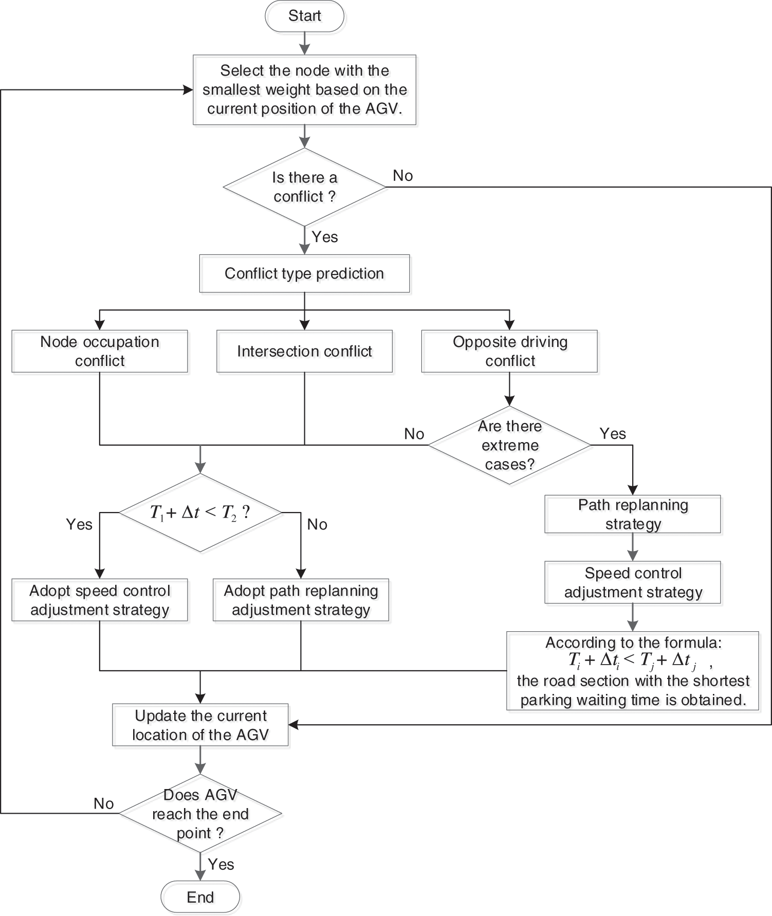
Figure 11: AGV conflict resolution process

4  Case Studies

4.1 Algorithm Verification

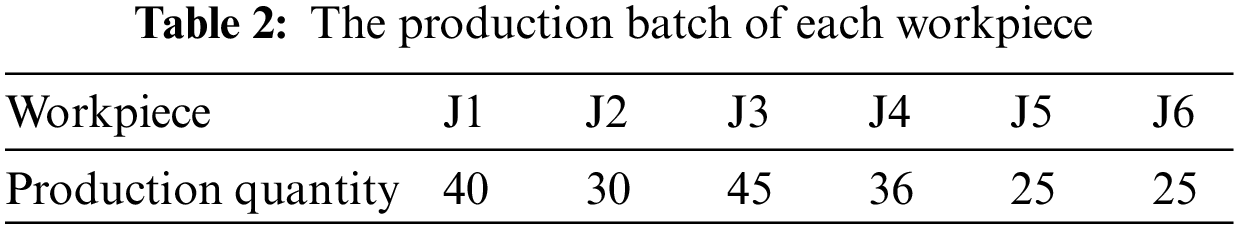
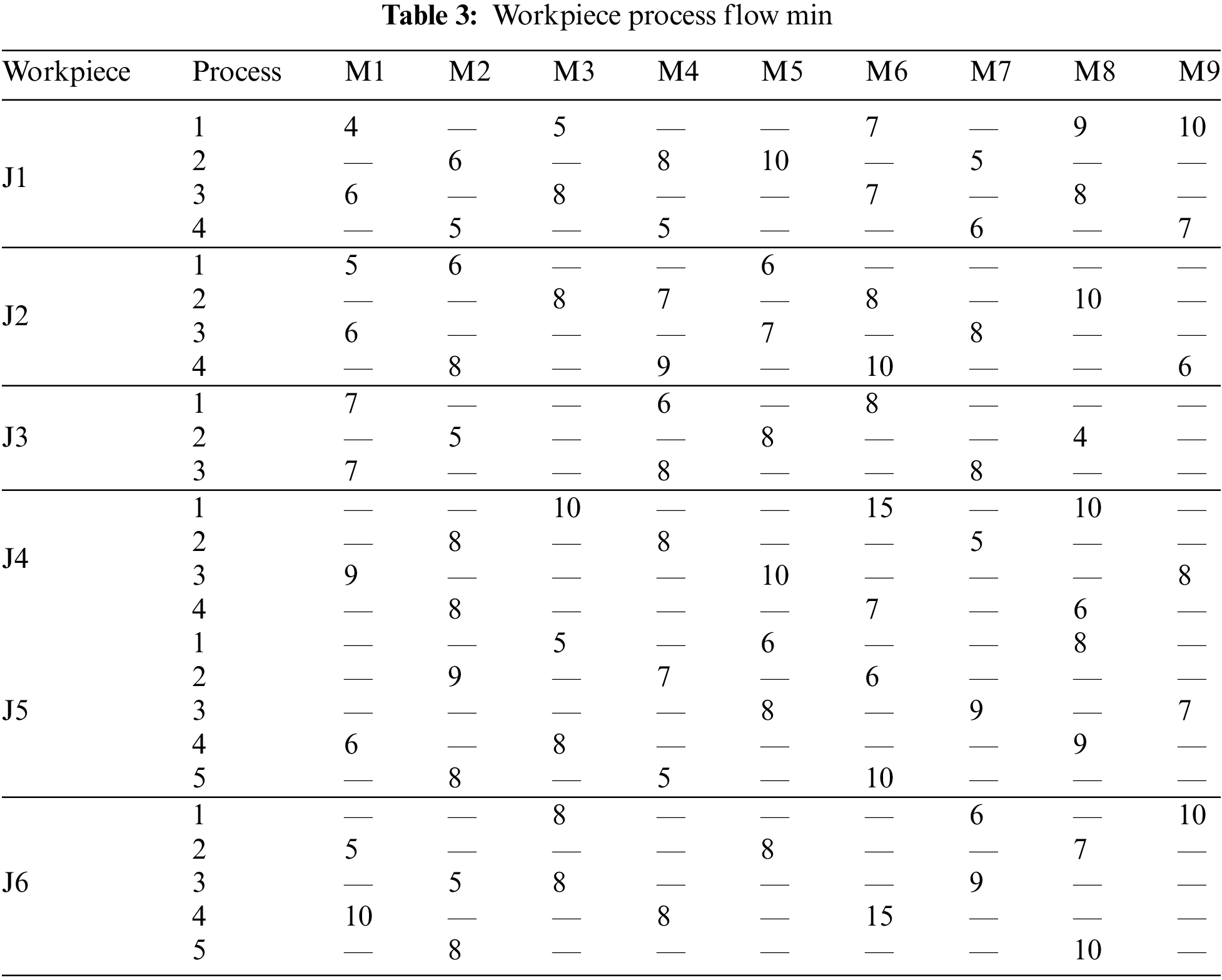
To verify the solution effect of the algorithm designed in this paper, the algorithm is tested with the actual production case 1: A machine shop has 9 machine tools and 2 AGVs which are responsible for the processing and transfer of production tasks, in which the driving speed of the AGV is 20m/min and the carrying capacity is 20 pieces. The layout of the shop and the nodes on the guide path is shown in Fig. 12. The shop needs to produce 6 kinds of workpieces and the production batch of each workpiece is shown in Table 2. The process flow of each workpiece is shown in Table 3, and “—” in the table means that this process cannot be processed on the corresponding machine.

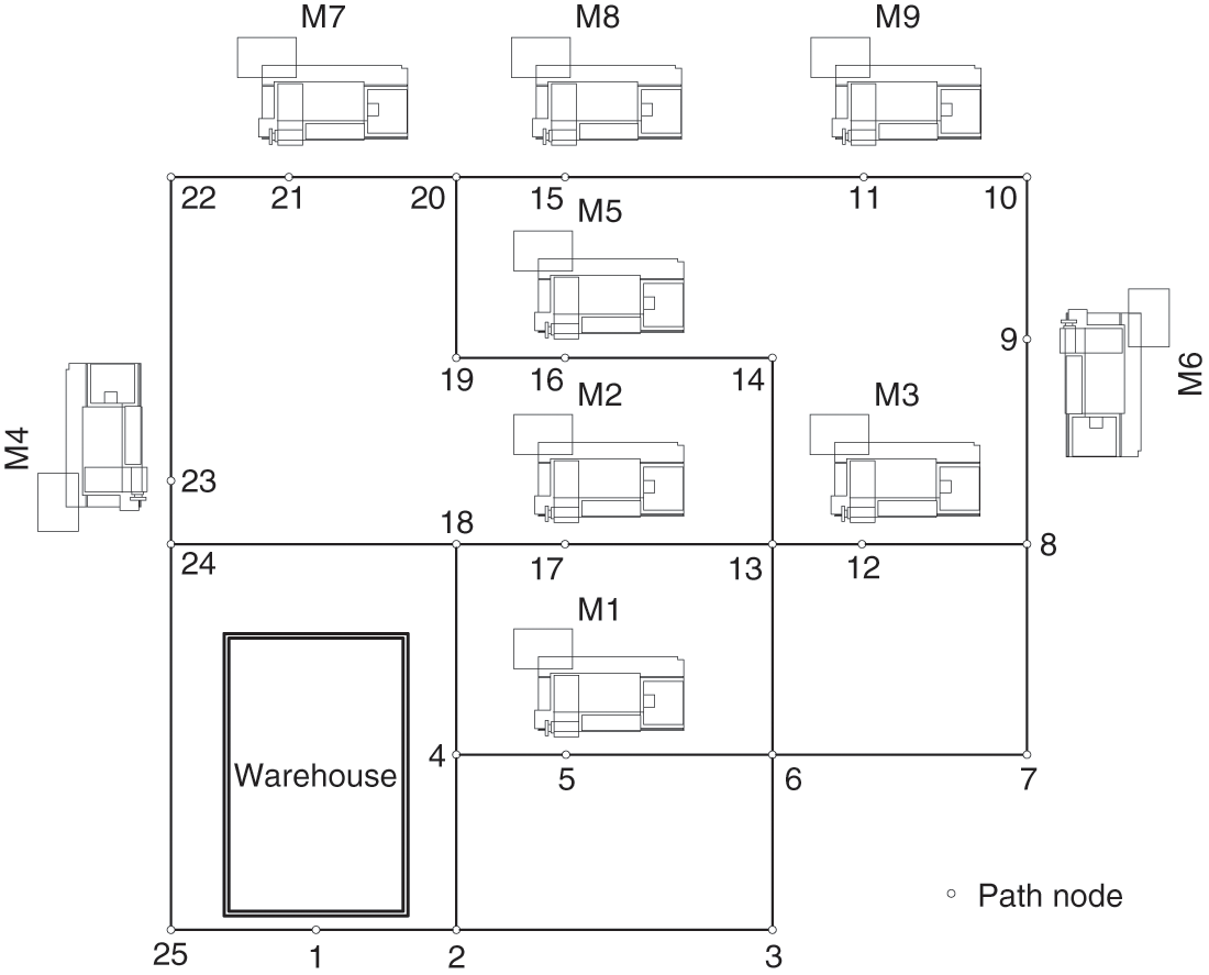
Figure 12: Workshop layout and guidance path diagram

(1) Parameter Sensitivity Analysis

To obtain the best performance of the multi-layer optimization algorithm, it is necessary to analyze the sensitivity of the disturbance threshold m of the algorithm and test the effectiveness of the optimization algorithm. The initial parameters of the algorithm are set below. The number of iterations of the outer algorithm of the improved nested optimization algorithm is 60, and the disturbance threshold m is 3. The number of iterations of the inner layer algorithm is 80, and the population size is 40. Different disturbance thresholds m are set under the initial parameter conditions, 10 consecutive calculations are set each time, and the best results of 10 times are taken to complete the sensitivity analysis of the parameters. Fig. 13 is the iterative curve when the disturbance threshold m is 2, 3, 4, 5, respectively.

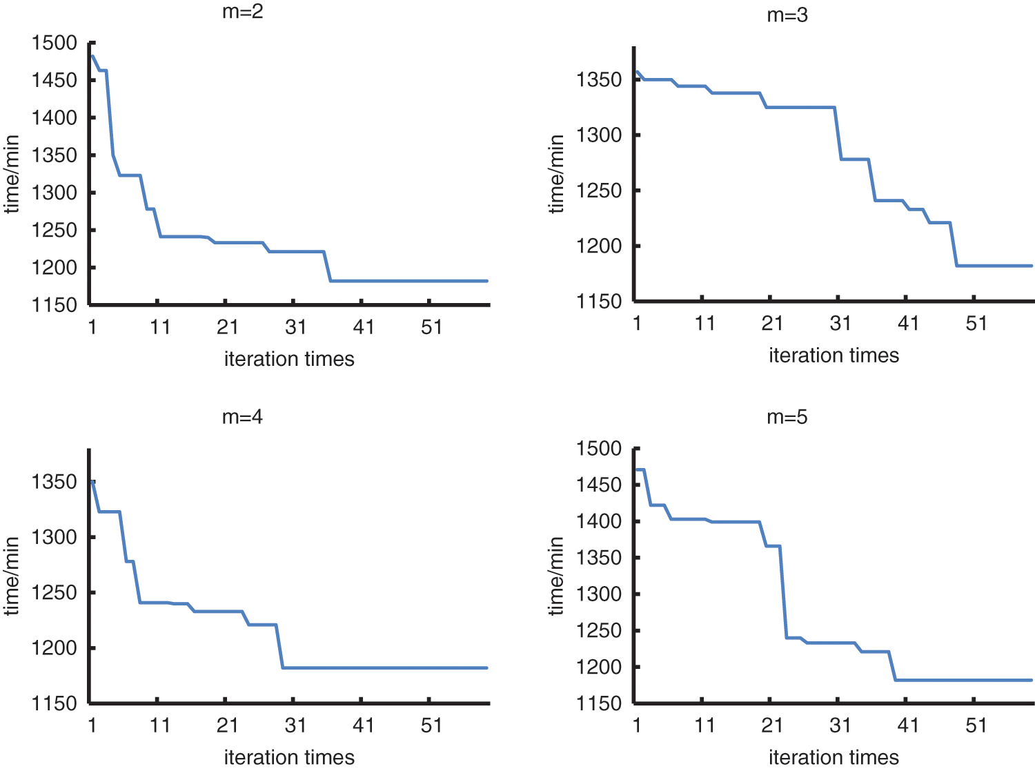
Figure 13: Iteration curves of different disturbance threshold m

It can be seen from the iterative curves of different disturbance thresholds m that when m takes different values, it has little effect on the results of the optimal scheme, but has a great influence on the convergence speed of the optimization algorithm. It can be seen from the figure that when m=2, the algorithm completes convergence in about 36 generations; when m=3, the algorithm completes convergence in about 48 generations; when m=4, the algorithm completes convergence in about 29 generations, and when m=5, the algorithm completes convergence in about 39 generations. It can be seen that when m=4, the optimization effect of the algorithm is better, so when solving the optimization scheme for subsequent production cases, the disturbance threshold m of the optimization algorithm is set to 4.

In addition, to obtain better solution results, the following sensitivity analysis is performed on the size of the population size. The above cases are solved by setting different population sizes. The experimental results are shown in Fig. 14. The experimental results show that with the increase in population size, the global search ability of the algorithm is enhanced, and the possibility of finding the global optimal solution is increased. However, when the population size exceeds 50, as the population size continues to increase, the global optimal solution searched remains stable, but the evolutionary algebra of the algorithm is reduced, which indicates that when the population size is set to 50, the algorithm has been able to find the global optimal solution in the solution space. Therefore, the optimal population size of this paper is set to 50.

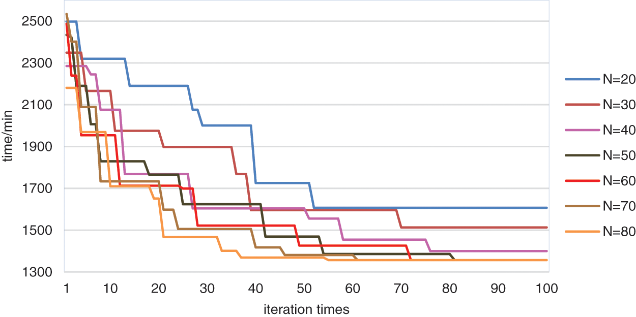
Figure 14: The influence of population size on algorithm performance

(2) Algorithm effectiveness test

The system solves the above case batching, scheduling, and path planning schemes with the minimum production cycle as the optimization objective. The number of iterations of the outer batch optimization algorithm is set to 80, and the perturbation threshold is set to 4; the number of iterations of the inner dual-resource scheduling algorithm is set to 100, and the population size is set to 50. The system solves the optimization results as follows: The completion time of the optimal solution is 1329 min. Table 4 shows the iteration results of the batch optimization solution; Table 5 is the optimal batching scheme; Table 6 shows the processing sequence of the three sub-batches of workpiece 2 in the optimal solution. Fig. 15 shows the iterative curve of the algorithm’s optimization target, and Fig. 16 shows the load time of the two production resources, machine tool, and AGV, in the optimal solution.

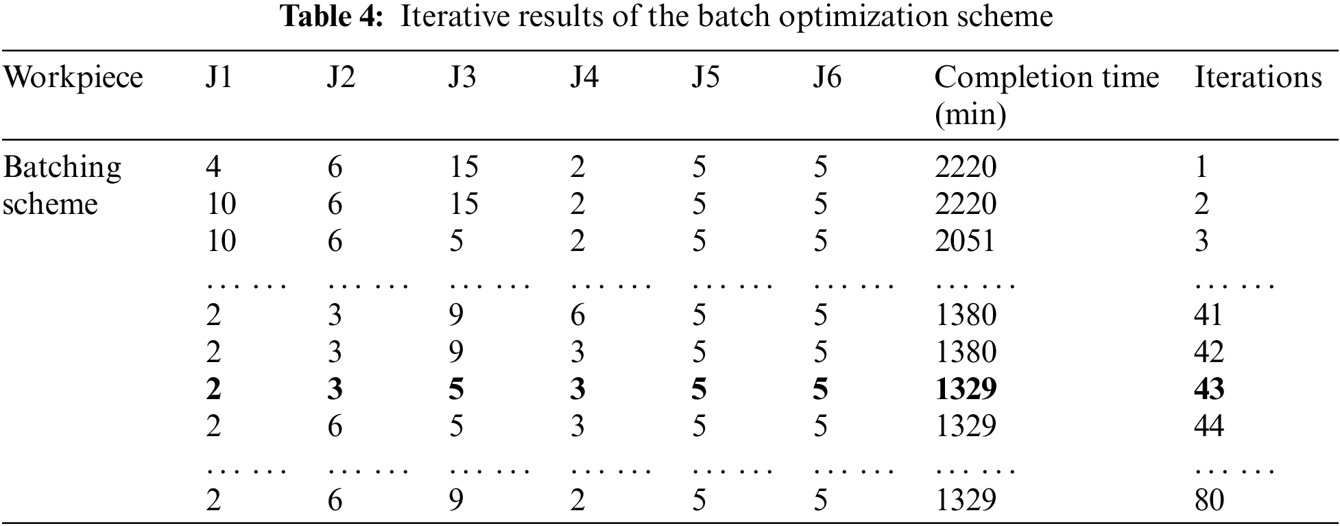
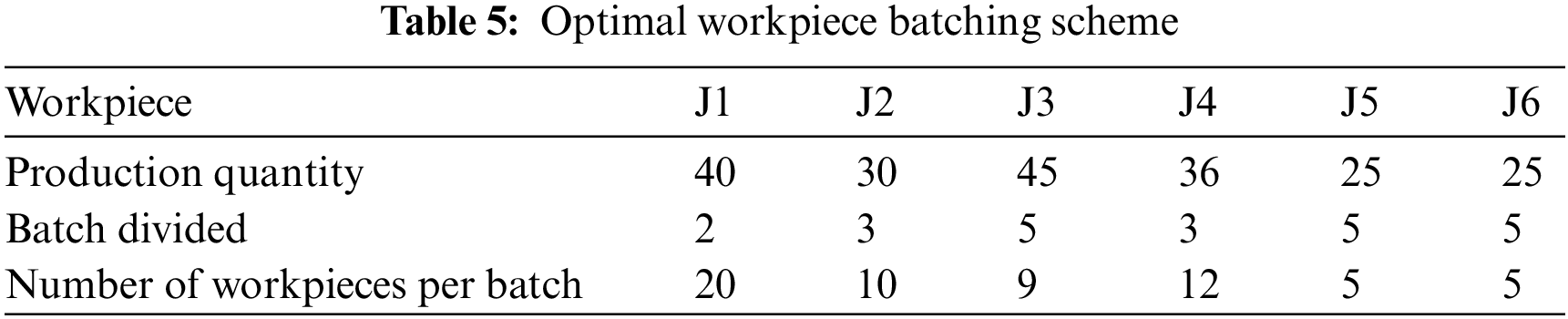
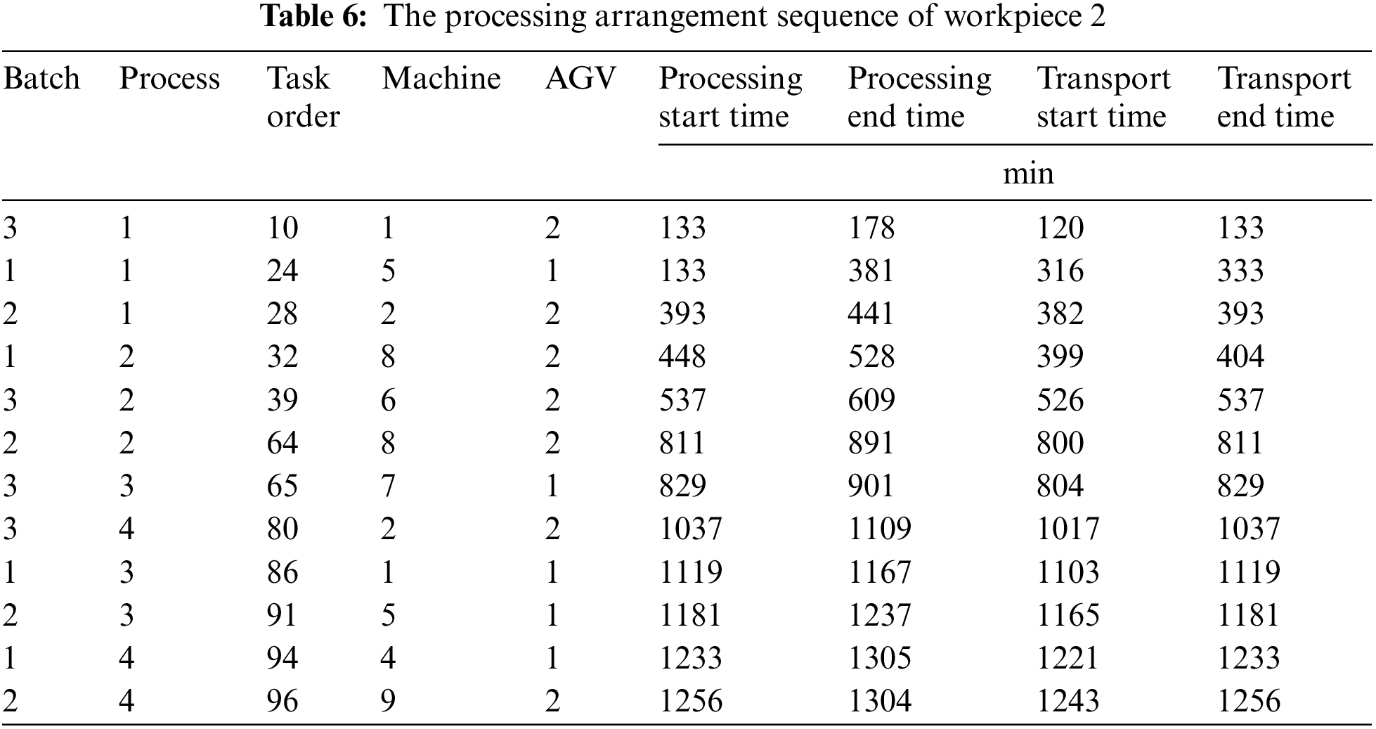
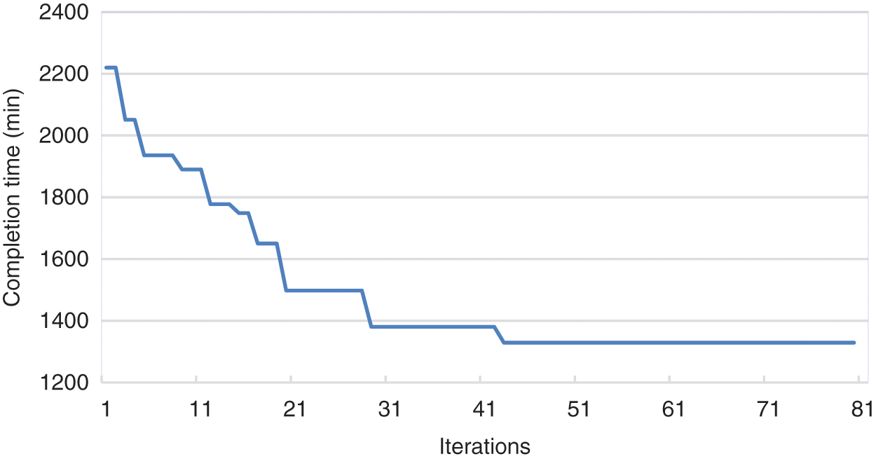
Figure 15: Iteration curve

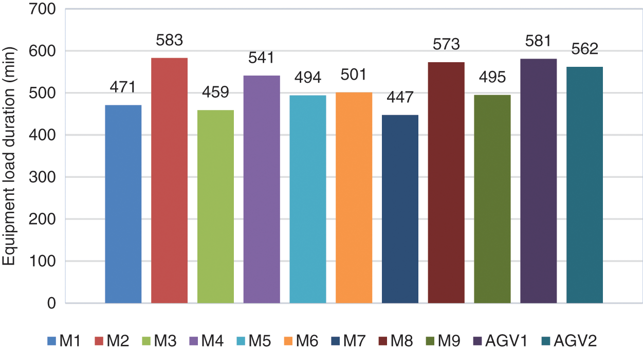
Figure 16: Equipment load duration

From the test results of the above example, it can be seen that the improved nested optimization algorithm designed in this paper can effectively solve the flexible workshop dual resource batch scheduling optimization problem. And the batch optimization scheme, dual resource scheduling scheme, and path scheme obtained from the solution can well guide the workshop production activities.

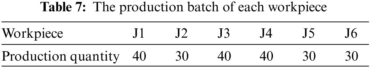
To verify the superiority of the improved nested optimization algorithm, the experimental analysis is carried out through the actual production case 2. Case 2 contains 5 kinds of workpieces. The production batch of each workpiece is shown in Table 7. The process flow of the workpiece is still shown in Table 3. The layout of the workshop is still shown in Fig. 12. There are 9 machine tools and 3 AGVs in the workshop to perform production tasks. The driving speed of AGV is 20 m/min, and the maximum single carrying capacity is 20 pieces.

The improved nested optimization algorithm (INOA) and the unimproved basic nested optimization algorithm (BNOA) were used to solve case 2 for 10 times respectively. The parameter settings of IBOA are the same as those of case 1. The crossover probability and mutation probability of BNOA are set at 0.95 and 0.05, and other basic parameters are consistent with INOA. The experimental results are shown in Table 8, and the result statistics of the two algorithms running 10 times are shown in Table 9 and Fig. 17. The optimal batching scheme of INOA and BNOA running 10 times each is shown in Table 10, and the optimal dual resource scheduling scheme is shown in Figs. 18 and 19, respectively.

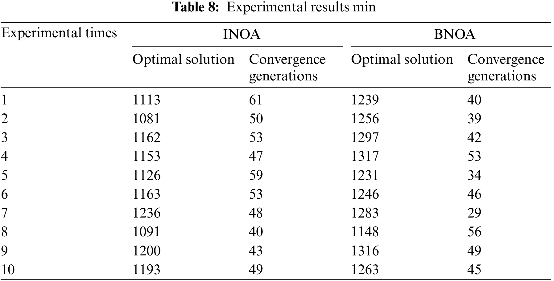
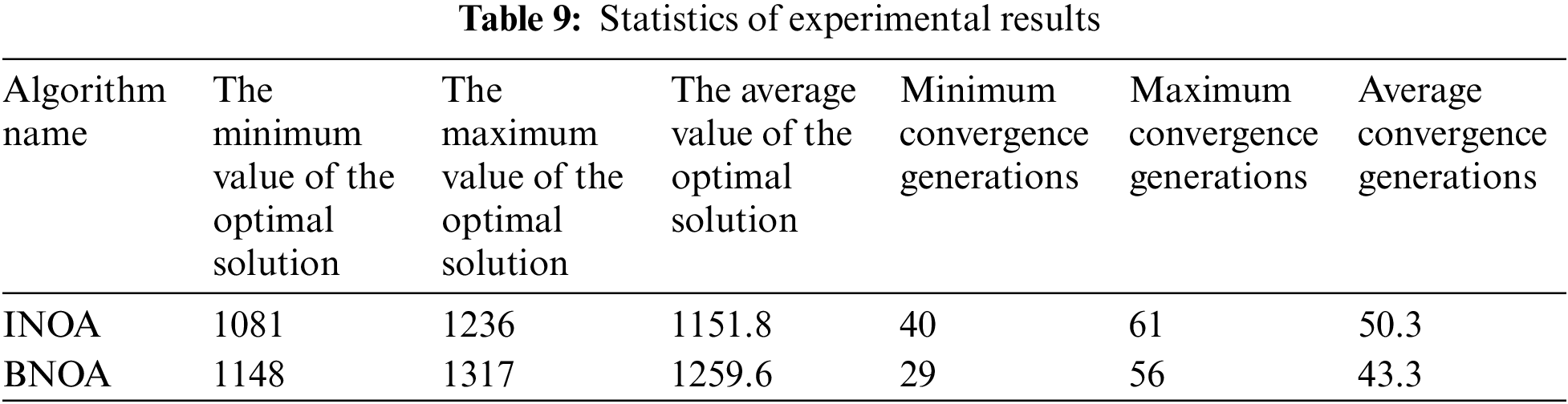
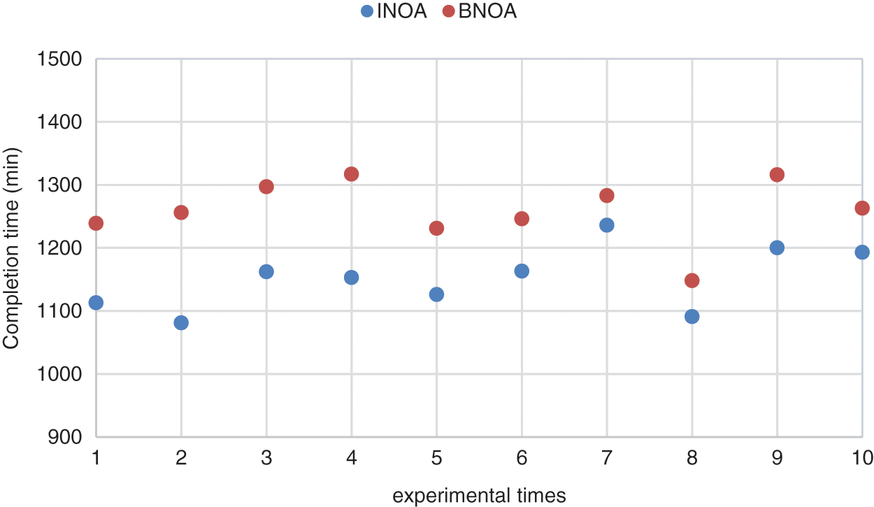
Figure 17: Optimal solution distribution scatter plot

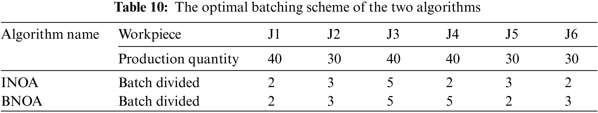
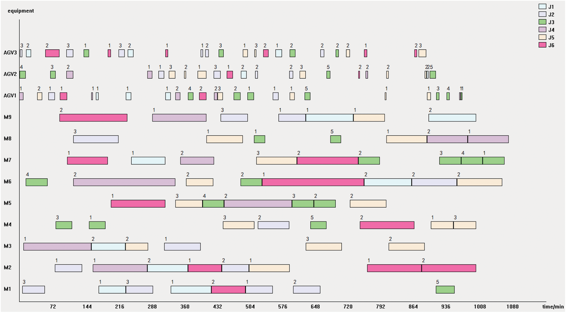
Figure 18: Gantt chart of the optimal dual resource scheduling scheme obtained by the INOA algorithm

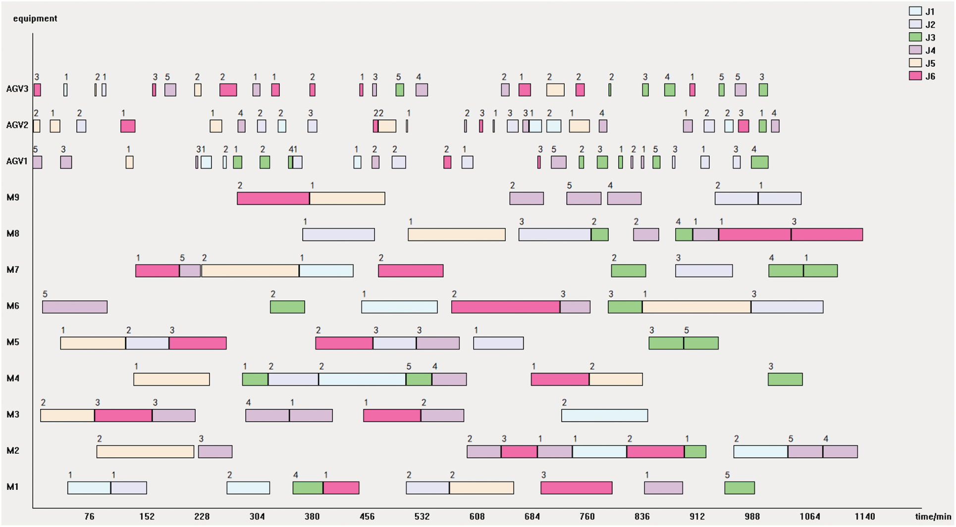
Figure 19: Gantt chart of the optimal dual resource scheduling scheme obtained by the BNOA algorithm

It can be seen from the above experimental results that the minimum value of the optimal solution of the INOA running 10 times is 1081 min, and the average value of the optimal solution is 1151.8 min. The minimum value of the optimal solution of the BNOA is 1148 min, and the average value of the optimal solution is 1259.6 min. The average value of the optimal solution of the INOA decreased by 8.6% compared to the BNOA, indicating that the solution effect of the INOA is significantly better than that of the unimproved BNOA. The convergence speed of the BNOA is faster than that of the INOA. This is because the BNOA is easy to fall into the local optimal solution in the iterative process, resulting in a relatively poor solving effect.

4.2 Analysis of AGV Configuration Quantity

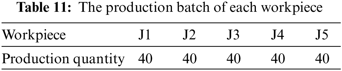
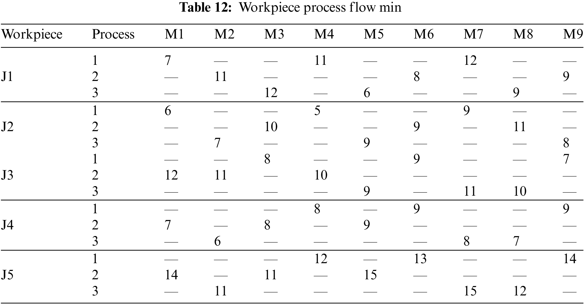
The actual production case 3 is used to analyze the influence of the number of AGV configurations on production efficiency. Case 3 contains 5 kinds of workpieces. The production batch of each workpiece is shown in Table 11; the process flow of the workpieces is shown in Table 12; the layout of the workshop is still shown in Fig. 12. The logistics solution of this workshop adopts a self-unloading backpacking roller-type AGV with a driving speed of 20 m/min and a carrying capacity of 20 pieces. By changing the configuration number of AGVs in case 3, the influence of different configuration numbers of AGVs on the workshop production cycle and equipment utilization rate is analyzed.

Figs. 20–22 respectively show the Gantt charts of the optimal dual-resource scheduling scheme for the cases with the number of AGV configurations of 2, 4, and 8, and the corresponding production cycles of 1340, 1107, and 916 min. It can be seen from the figures, as the number of AGVs increases, the Gantt chart of the transfer task of AGVs is gradually sparse throughout the production cycle, while the Gantt chart of the machine tool processing task is gradually compact throughout the production cycle, which indicates that with the increase of the number of AGVs, the machine tool utilization is significantly improved and the production cycle is significantly shortened.

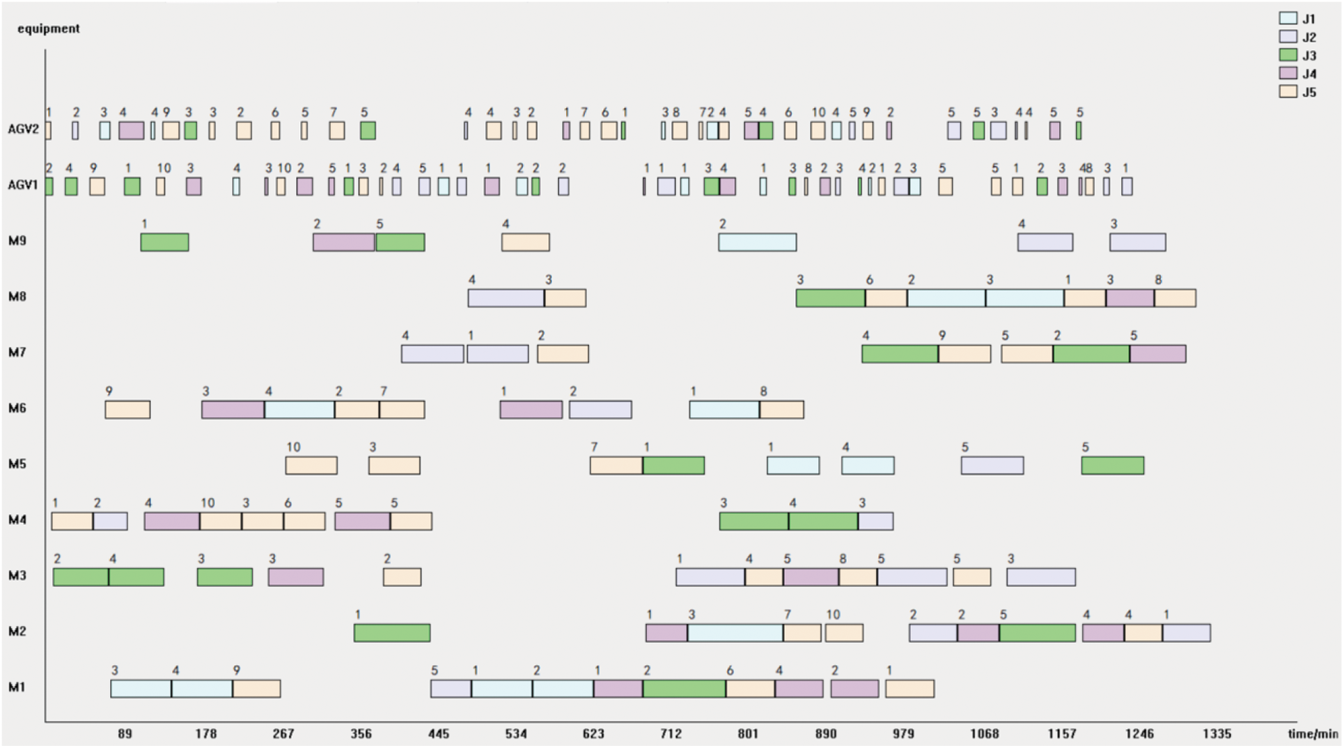
Figure 20: Scheduling scheme with 2 AGVs

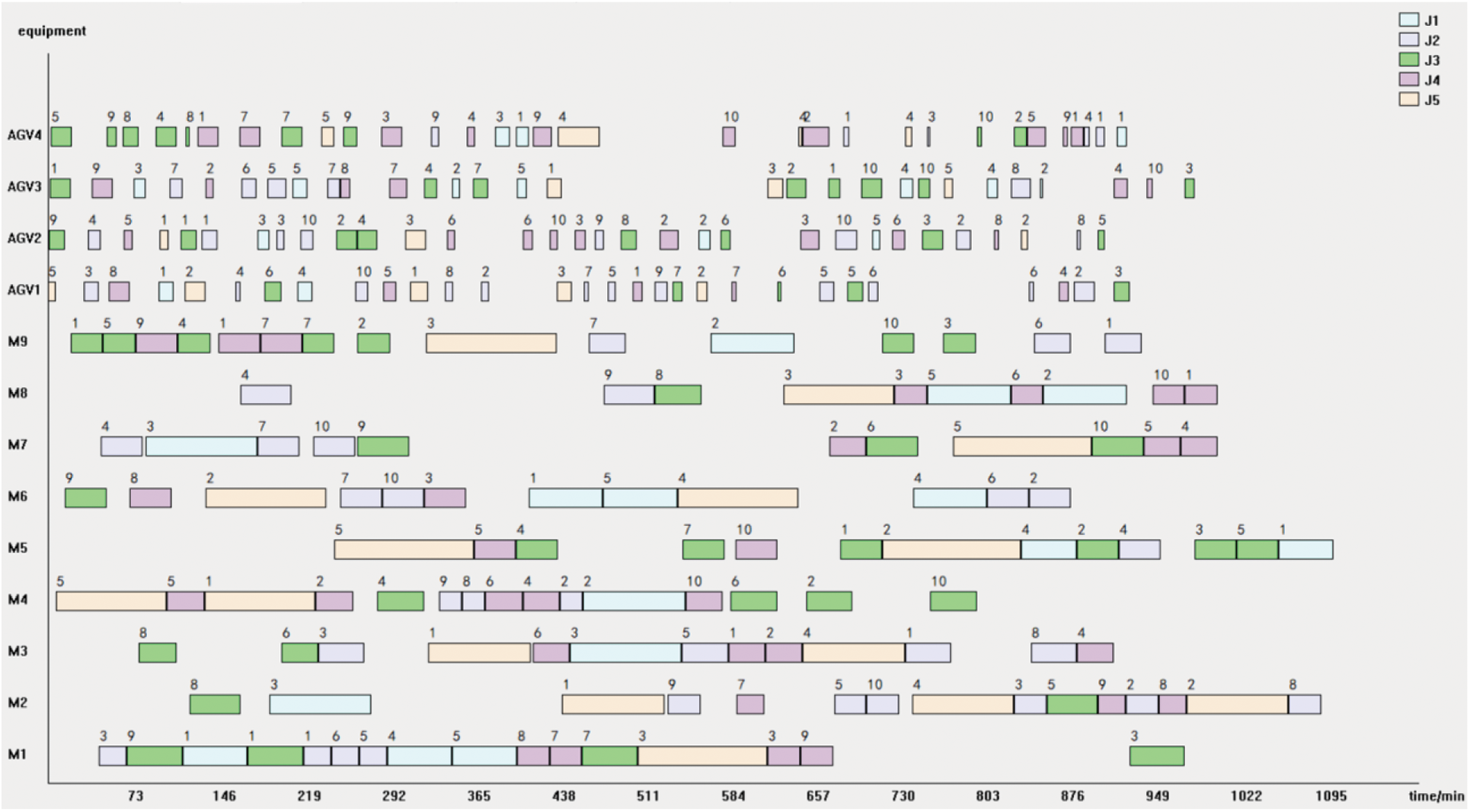
Figure 21: Scheduling scheme with 4 AGVs

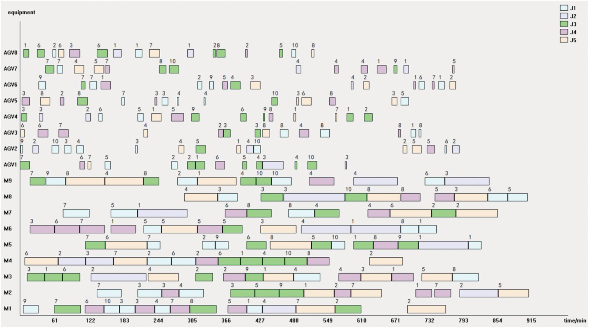
Figure 22: Scheduling scheme with 8 AGVs

Tables 13 and 14 show the statistical results of various types of data in the workshop with different numbers of AGV configurations. Five simulations are performed for each AGV configuration. The completion time is taken as the result of the optimal solution; the average machine load is the average load of the 9 machines of the optimal solution in the 5 simulations; the utilization rate is the percentage of the average load and the completion time. The average load and the utilization rate of AGVs are the same as the machine statistics method.

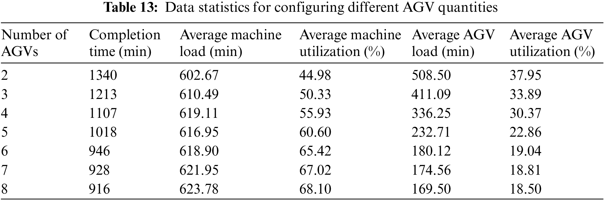
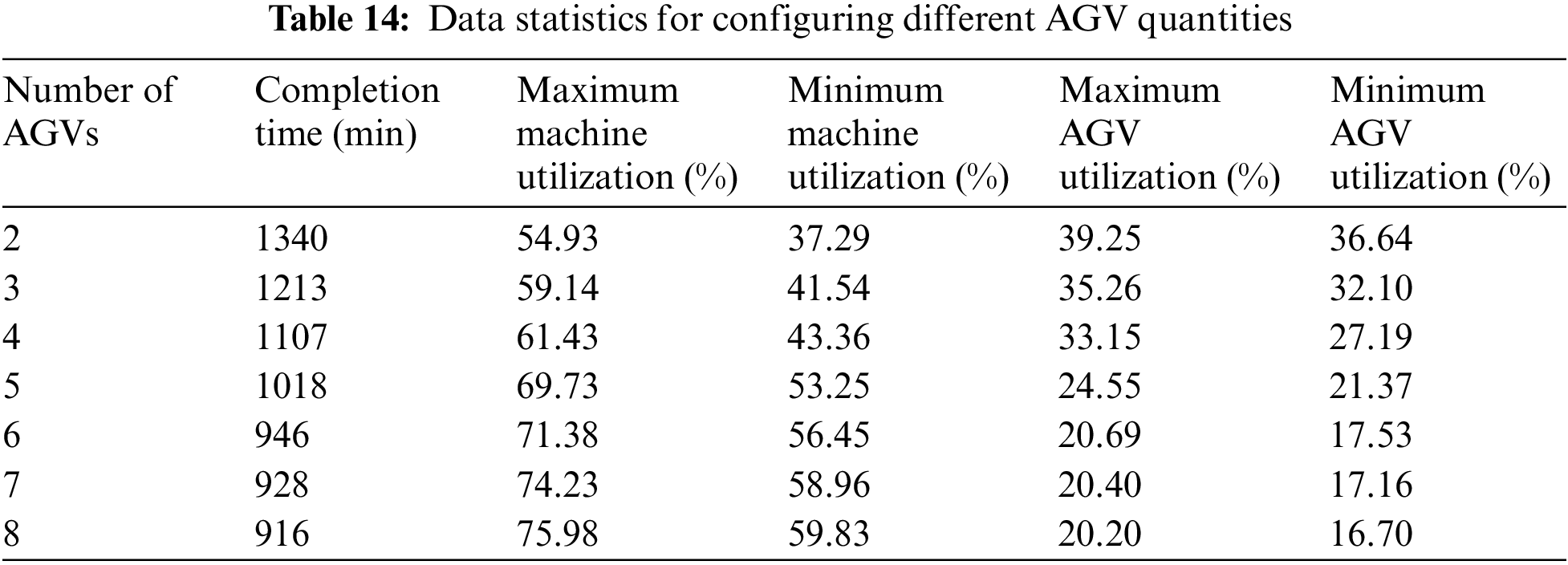
Fig. 23 shows the influence of AGV configuration quantity on completion time and equipment utilization.

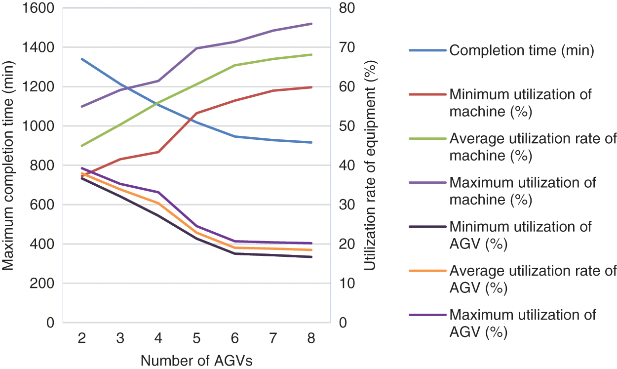
Figure 23: Influence diagram of AGV configuration quantity

From Tables 13, 14, and Fig. 23, it can be seen that as the number of AGVs increases, the production cycle of the workshop is gradually shortened; the utilization rate of machine tools gradually increases, but the utilization rate of AGVs gradually decreases; and after the number of AGVs reaches 6, the increasing the number of AGVs has negligible effects on the completion time, machine tools and utilization rate of AGVs. The relationship between the number of AGVs and the production efficiency of the workshop is consistent with the law of diminishing border effect. Therefore, the workshop needs to consider the impact of maintenance cost and completion time of the different numbers of AGVs on the workshop efficiency when facing the different scales of production.

5  Conclusion

In this paper, the batch optimization of workshop products, dual resource scheduling optimization, and collision-free path planning problem of AGVs are studied; a mathematical model is established with the minimum production cycle as the optimization objective; and an improved nested optimization algorithm is designed based on a variety of improved optimization algorithms. The algorithm is tested through actual cases, and the impact of different AGV configuration quantities on production efficiency is analyzed through case simulation, and the number of AGV configurations and the workshop production efficiency are in line with the boundary decreasing law. The test results show that the improved nested optimization algorithm designed in this paper can effectively achieve the solution of integrated optimization problems of batch optimization, dual resource scheduling optimization, and AGV collision-free path optimization for the flexible workshop, and can provide intellectual support for the decision-making service of the intelligent workshop.

Although this paper has completed the solution of the dual-resource batch scheduling optimization problem for the flexible job shop and the iterative optimization of the designed improved nested optimization algorithm that can solve the optimized scheduling scheme, several aspects are simplified in building the model. Further optimization can be solved according to the actual workshop production process in the future by considering various optimization objectives such as equipment utilization, production energy consumption, processing cost, etc. Moreover, emergency order insertion, equipment failure, and other unexpected disturbance events may occur in the workshop during processing, and it is necessary to study rescheduling or dynamic scheduling to solve the disturbance events occurring in the production process.

Funding Statement: The authors received no specific funding for this study.

Conflicts of Interest: The authors declare that they have no conflicts of interest to report regarding the present study.

References

1. T. Zhang, Q. Li, C. S. Zhang, H. W. Liang, P. Li et al., “Current trends in the development of intelligent unmanned autonomous systems,” Frontiers of Information Technology & Electronic Engineering, vol. 18, no. 1, pp. 68–85, 2017. [Google Scholar]

2. Y. Li, Z. M. Wu and Q. Gan, “Integrated scheduling of machines and AGVs in flexible manufacturing environment,” China Mechanical Engineering, vol. 12, no. 4, pp. 447–450, 2001. [Google Scholar]

3. C. Z. He, Y. C. Song, Q. Lei, X. F. Lyu, R. X. Liu et al., “Integrated scheduling of multiple AGVs and machines in flexible job shops,” China Mechanical Engineering, vol. 30, no. 4, pp. 438–447, 2019. [Google Scholar]

4. Y. Q. Xu, C. M. Ye and L. Cao, “Research on flexible job-shop scheduling problem with AGV constraints,” Application Research of Computers, vol. 35, no. 11, pp. 3271–3275, 2018. [Google Scholar]

5. X. X. Li, D. M. Yang, X. Li and R. Wu, “Flexible job shop AGV fusion scheduling method based on HGWOA,” China Mechanical Engineering, vol. 32, no. 8, pp. 938–950+986, 2021. [Google Scholar]

6. Q. H. Liu, N. J. Wang, J. Li, T. T. Ma, F. P. Li et al., “Research on flexible job shop scheduling optimization based on segmented AGV,” Computer Modeling in Engineering & Sciences, vol. 134, no. 3, pp. 2073–2091, 2023. [Google Scholar]

7. K. Chen, L. Bi and W. Y. Wang, “Research on integrated scheduling of AGV and machine in flexible job shop,” Journal of System Simulation, vol. 34, no. 3, pp. 461–469, 2022. [Google Scholar]

8. A. B. N. Paksi and A. Ma’Ruf, “Flexible job-shop scheduling with dual-resource constraints to minimize tardiness using genetic algorithm,” IOP Conference Series Materials Science and Engineering, vol. 114, no. 1, pp. 012060, 2016. [Google Scholar]

9. H. C. Li and H. D. Zhu, “Modified water wave optimization for energy-conscious dual-resource constrained flexible job shop scheduling,” International Journal of Performability Engineering, vol. 16, no. 6, pp. 916–929, 2020. [Google Scholar]

10. S. Zhang, H. T. Du, S. Borucki, S. F. Jin, T. T. Hou et al., “Dual resource constrained flexible job shop scheduling based on improved quantum genetic algorithm,” Machines, vol. 9, no. 6, pp. 108, 2021. [Google Scholar]

11. B. Z. Xu, X. L. Fei and X. L. Zhang, “Batch division and parallel scheduling optimization of flexible job shop,” Computer Integrated Manufacturing Systems, vol. 22, no. 8, pp. 1953–1964, 2016. [Google Scholar]

12. J. P. Xu, G. M. Lu, P. Yu and Q. R. He, “Robust multi-objective flexible job shop scheduling with batch startup time,” Modern Manufacturing Engineering, vol. 10, pp. 28–34, 2019. [Google Scholar]

13. X. H. Liu, C. Duan and L. Wang, “Flexible job shop scheduling with lot streaming based on improved migrating birds optimization algorithm,” Computer Integrated Manufacturing Systems, vol. 27, no. 11, pp. 3185–3195, 2021. [Google Scholar]

14. C. Tan, J. H. Zhang and T. Guo, “Multi-objective flexible job shop scheduling considering lot-splitting,” Modern Manufacturing Engineering, vol. 12, pp. 25–35, 2020. [Google Scholar]

15. A. Bozek and F. Werner, “Flexible job shop scheduling with lot streaming and sublot size optimization,” International Journal of Production Research, vol. 56, no. 19, pp. 6391–6411, 2018. [Google Scholar]

16. R. H. Huang and T. H. Yu, “An effective ant colony optimization algorithm for multi-objective job-shop scheduling with equal-size lot-splitting,” Applied Soft Computing Journal, vol. 57, pp. 642–656, 2017. [Google Scholar]

17. X. L. Wu, J. J. Peng, Z. R. Xie, N. Zhao and S. M. Wu, “An improved multi-objective optimization algorithm for solving flexible job shop scheduling problem with variable batches,” Journal of Systems Engineering and Electronics, vol. 32, no. 2, pp. 272–285, 2021. [Google Scholar]

18. Z. H. Jia, Y. Wang, C. Wu, Y. Yang, X. Y. Zhang et al., “Multi-objective energy-aware batch scheduling using ant colony optimization algorithm,” Computers and Industrial Engineering, vol. 131, no. 4, pp. 41–56, 2019. [Google Scholar]

19. Q. Zeng, L. Shen, H. Ren and L. Y. Wu, “Multi-objective scheduling method for batch production FJSP with dual-resource,” Computer Engineering and Applications, vol. 51, no. 1, pp. 250–256, 2015. [Google Scholar]