
 Submit a Paper
 Propose a Special lssue
 Open Access
ARTICLE

Deep-Net: Fine-Tuned Deep Neural Network Multi-Features Fusion for Brain Tumor Recognition
1 Department of Computer Science, HITEC University, Taxila, 47080, Pakistan
2 Department of Informatics, University of Leicester, Leicester, UK
3 Information Systems Department, Faculty of Computers and Information Sciences, Mansoura University, Mansoura, Egypt
4 Department of Computer Engineering, College of Computer Science, King Khalid University, Abha, 61413, Saudi Arabia
5 Computer Sciences Department, College of Computer and Information Sciences, Princess Nourah bint Abdulrahman University, Riyadh, 11671, Saudi Arabia
6 Management Information System Department, College of Business Administration, Prince Sattam Bin Abdulaziz University, Al-Kharj, 16278, Saudi Arabia
7 Department of Computer Science, Hanyang University, Seoul, 04763, Korea
* Corresponding Author: Jaehyuk Cha. Email:
Computers, Materials & Continua 2023, 76(3), 3029-3047. https://doi.org/10.32604/cmc.2023.038838
Received 30 December 2022; Accepted 23 May 2023; Issue published 08 October 2023
 View Full Text
 Download PDF
Abstract
Manual diagnosis of brain tumors using magnetic resonance images (MRI) is a hectic process and time-consuming. Also, it always requires an expert person for the diagnosis. Therefore, many computer-controlled methods for diagnosing and classifying brain tumors have been introduced in the literature. This paper proposes a novel multimodal brain tumor classification framework based on two-way deep learning feature extraction and a hybrid feature optimization algorithm. NasNet-Mobile, a pre-trained deep learning model, has been fine-tuned and two-way trained on original and enhanced MRI images. The haze-convolutional neural network (haze-CNN) approach is developed and employed on the original images for contrast enhancement. Next, transfer learning (TL) is utilized for training two-way fine-tuned models and extracting feature vectors from the global average pooling layer. Then, using a multiset canonical correlation analysis (CCA) method, features of both deep learning models are fused into a single feature matrix—this technique aims to enhance the information in terms of features for better classification. Although the information was increased, computational time also jumped. This issue is resolved using a hybrid feature optimization algorithm that chooses the best classification features. The experiments were done on two publicly available datasets—BraTs2018 and BraTs2019—and yielded accuracy rates of 94.8% and 95.7%, respectively. The proposed method is compared with several recent studies and outperformed in accuracy. In addition, we analyze the performance of each middle step of the proposed approach and find the selection technique strengthens the proposed framework.Keywords
Cancer is rapidly becoming a major public health concern worldwide [1]. It is the second leading cause of death after cardiovascular disease, accounting for one out of every six deaths worldwide [2]. Brain cancer is one of the deadliest diseases due to its violent nature, low survival rate, and diverse features. Tumor shape, texture, and location are some of the different features that can be used to classify brain tumors [3]. Meningiomas are the most common benign intracranial tumors that inflame the thin membranes surrounding the brain and spinal cord. Astrocytomas, ependymomas, glioblastomas, oligoastrocytomas, and oligodendrogliomas are all types of brain tumors known as gliomas [4]. Pituitary tumors, which develop at the pituitary gland’s base in the brain, are frequently benign. However, these lesions may prevent the generation of pituitary hormones, which would have a systemic impact [5].
In medical care, the incidence rates of meningiomas, gliomas, and pituitary tumors are about 15%, 45%, and 15%, respectively [6]. Physicians may diagnose and predict a patient’s survival rate based on the type of tumor. At the same time, the best treatment method, from surgery, chemotherapy, or radiotherapy to the “wait and see” strategy that ignores invasive procedures, can also be agreed upon. Classification of the tumor is vital for planning and monitoring the course of treatment [7]. MRI is a non-invasive, painless medical imaging technique. It is one of the most accurate detection and classification techniques for cancer. A radiologist’s knowledge is required for the highly technical, error-prone, and time-consuming task of identifying the type of malignancy from MRI scans. In the artificial intelligence (AI) area, a new and creative computer assistant diagnostic (CAD) system is urgently required to enable doctors and radiologists to ease the workload of diagnosing and classifying tumors.
A CAD system typically consists of three steps denoted (1) tumor segmentation, (2) extraction of the segmented tumor’s characteristics based on statistical or mathematical parameters evaluated throughout the learning process using a collection of MRI images that are labeled, and (3) implementing an accurate machine learning classifier to estimate an anomaly class [8]. Before the classification stage, many conventional machine learning (ML) approaches are required for lesion identification [9]. The segmentation process is a computationally intensive phase, which might be unpredictable according to image contrast and intensity normalization variance and can influence classification performance. Feature extraction is a critical method of producing interesting features to identify a raw image’s contents. However, this phase has few adverse effects of being a time-consuming assignment requiring prior knowledge of the problem domain. The extracted features are then utilized as ML inputs and assigned an image class label according to these crucial features [10]. Alternatively, deep learning (DL) is a subfield of artificial intelligence (AI) that automatically learns data representation and makes predictions and conclusions [11]. DL is independent of hand-crafted feature extraction methods and can learn features directly from the sample data through several hidden layers. Convolutional, ReLu activation, and pooling layers to avoid overfitting normalization, fully connected, and softmax layers are among the hidden layers in a straightforward convolutional neural network (CNN) model. The completely linked layer is the most crucial layer in which characteristics are obtained in 1D for classification purposes.
Deep learning models already pre-trained include Alexnet, VGG16, ResNet, and NasNet-Mobile. Compared to previous models, the NasNet-Mobile is lighter and performs better while analyzing medical images. Transfer learning (TL) is used to fine-tune and train the pre-trained deep models on the target dataset. The TL is a method of recycling a model with the least memory and computation required [12]. Later, some activation functions are employed on the newly trained feature extraction models, such as sigmoid or tanh. Generally, these deep learning models are trained using raw images without any region of interest (ROI) detection; therefore, there is a high chance of irrelevant and redundant feature extraction. The researchers try to resolve this issue by introducing some feature selection techniques. The feature selection is the optimal subset selection method from the original feature set. A few famous feature selection techniques employed in medical imaging are mouth flame, the t-distribution stochastic neighborhood approach (t-SNE) approach, correlation, etc. Sometimes, the feature extraction from one type of data does not give better results; therefore, researchers introduced several feature fusion techniques. As a result, they have improved the accuracy through feature fusion techniques but faced a limitation of high computational time [13].
Deepak et al. [14] suggested a CNN via transfer learning framework for classifying brain tumors. They utilized a pre-trained GoogleNet model and extracted features through TL. The extracted features were subsequently classified utilizing machine learning classifiers that improved classification accuracy. The main observation of this work was the ability of TL for fewer training images. Mohsen et al. [15] designed a classifier based on CNN for brain tumor classification. They used discrete wavelet transform and principal component analysis (PCA) to combine the features of CNN in the designed classifier. Sharif et al. [16] presented an end-to-end system for brain tumor classification. They used the Densenet201 pre-trained model to extract features that were later refined through two feature selection techniques called entropy-Kurtosis and modified GA. The selected features are merged utilizing the non-redundant serial-based approach and then employed as input to the classifiers for final classification. The observation of this study was the selection of the best features to reduce the computational time of the classifiers and enhance the classification accuracy. An automatic brain tumor segmentation method in 3D medical images was proposed by Kamnitsas et al. [17]. The two main parts mainly describe this method for the 3D CNN’s extremely accurate soft segmentation and, more importantly, for the 3D CRF’s post-processing of the created soft segmentation labels, which successfully produces the hard segmentation labels and eliminates false positives. The model offers more effective performance and has been tested on the BraTs2015 and ISLES 2015 datasets. An entirely automatic model for segmenting 3D tumor photos was proposed by Alqazzaz et al. [18]. They trained four SegNet models for analysis, and post-processing combined the data from those models. The original images’ maximum intensity information is encrypted to deep features for improved representation. This work categorizes the extracted features using the decision tree as a classifier.
On BraTs2017, experiments are conducted to arrive at an average F1 score of 0.80. A multimodal automatic brain tumor classification technique utilizing deep learning was presented by Khan et al. [19]. The model was based on performing the following task sequentially as follows: Linear contrast stretching; transfer learning-based features extraction utilizing pre-trained CNN models (VGG16 & VGG19); features selection based on correntropy; and finally, the classification of brain cancers using a fused matrix sent to the extreme learning machine (ELM). A deep learning model for brain tumor segmentation by merging short-term memory (LSTM) and co-evolutionary neural networks (ConvNet) concepts was introduced by Iqbal et al. [20]. Following pre-processing, the class-weighting concept is presented to solve the problems with class inequality. ConvNet produced a single score (exactitude) of 75% using the BraTS 2018 benchmark dataset, while an LSTM-based network generated 80% of the results with an overall fusion accuracy of 82.29 percent. Few other recent techniques are also introduced for brain tumor classification such as DarkNet-Color Map Superpixels [21], Exemplar Deep Features [22], and named a few more [23] (summary is seen in Table 1).

The techniques mentioned above focused on the fusion of deep learning features and selecting the optimal or best features from multimodal brain tumor classification. However, in the fusion process, they mainly focused on the accuracy of a classification and computational time. Moreover, the major challenge is accurately classifying tumor categories such as T1, T1CE, T2, and Flair. Each class has a high similarity in shape and texture; therefore, it is not easy to classify correctly. Another challenge is the high computational time that can be resolved using feature optimization techniques. In this work, we proposed a two-way deep learning features extraction and hybrid feature optimization algorithm-based best feature selection framework for brain tumor classification. Our major efforts and contributions to this work are listed as follows:
• A two-way deep learning framework is introduced and trained using transfer learning. Then, the trained deep learning framework’s average pooling layers are used to extract features.
• A multiset canonical correlation analysis (MCCA)-based features fusion technique is employed to get better information for accurate classification.
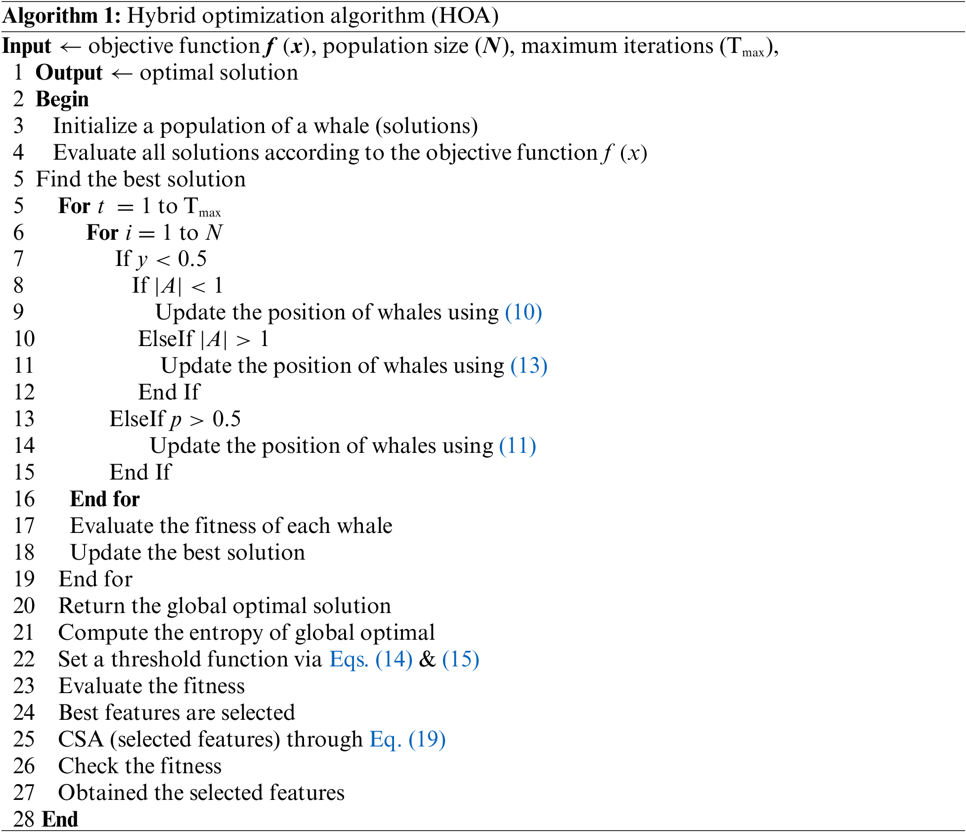
• We proposed a hybrid enhanced whale optimization algorithm with crow search (HWOA-CSA) to select the best feature and reduce the computational time.
• A comparison is conducted among the middle steps of the proposed framework. Also, we evaluated by comparing the proposed framework’s accuracy with recent state-of-the-art (SOTA) techniques.
The proposed methodology of this work, which includes a two-way deep learning framework for a hybrid feature optimization algorithm, is mentioned in Section 2. At the same time, detailed experimental results are shown in Section 3. Finally, we conclude the proposed framework in Section 4.
The proposed two-way deep learning model and optimal feature selection framework consist of a few important steps, as illustrated in Fig. 1. In the first step, a deep two-way learning fine-tuned model is trained on original and enhanced images. The main purpose is to obtain the most important features for accurate classification results. In the second step, fine-tuned networks are trained through TL and extracted features from average pooling layers. The extracted average pooling layer features are fused using a multiset CCA-based approach in the third step. In the next step, a hybrid HWOA-CSA feature selection algorithm is proposed and applied to a fused feature vector that is finally classified using an ELM classifier. The description of each step is given below.
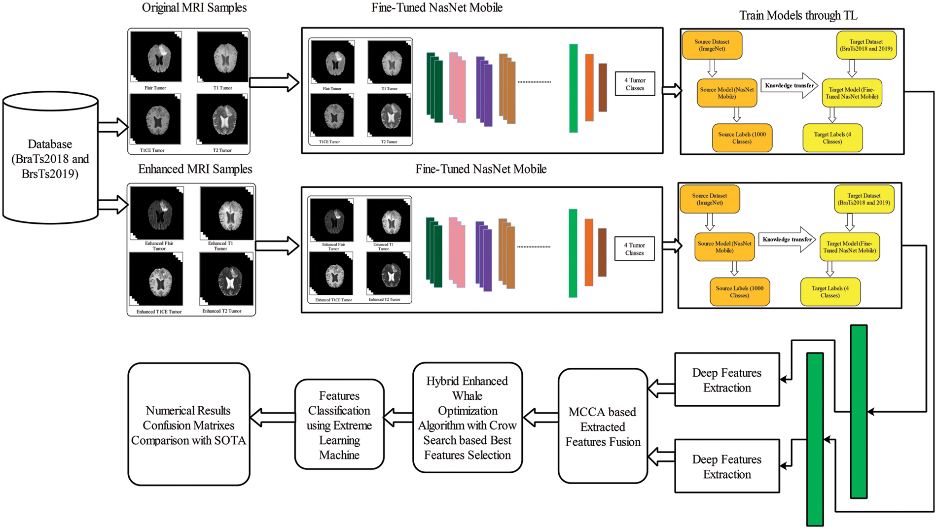
Figure 1: Architecture of proposed framework of multimodal brain tumor classification
2.1 Dataset Preparation and Contrast Enhancement
In this work, two datasets–BraTs2018 and BraTs2019, are employed for the experimental process. Both datasets consist of four types of tumor classes such as T1, T1W, T2, and FLAIR.
BraTs2018 [31]: This dataset consists of 385 scans for training and 66 scans for its validation. All the MRI scans of this dataset have a volume of
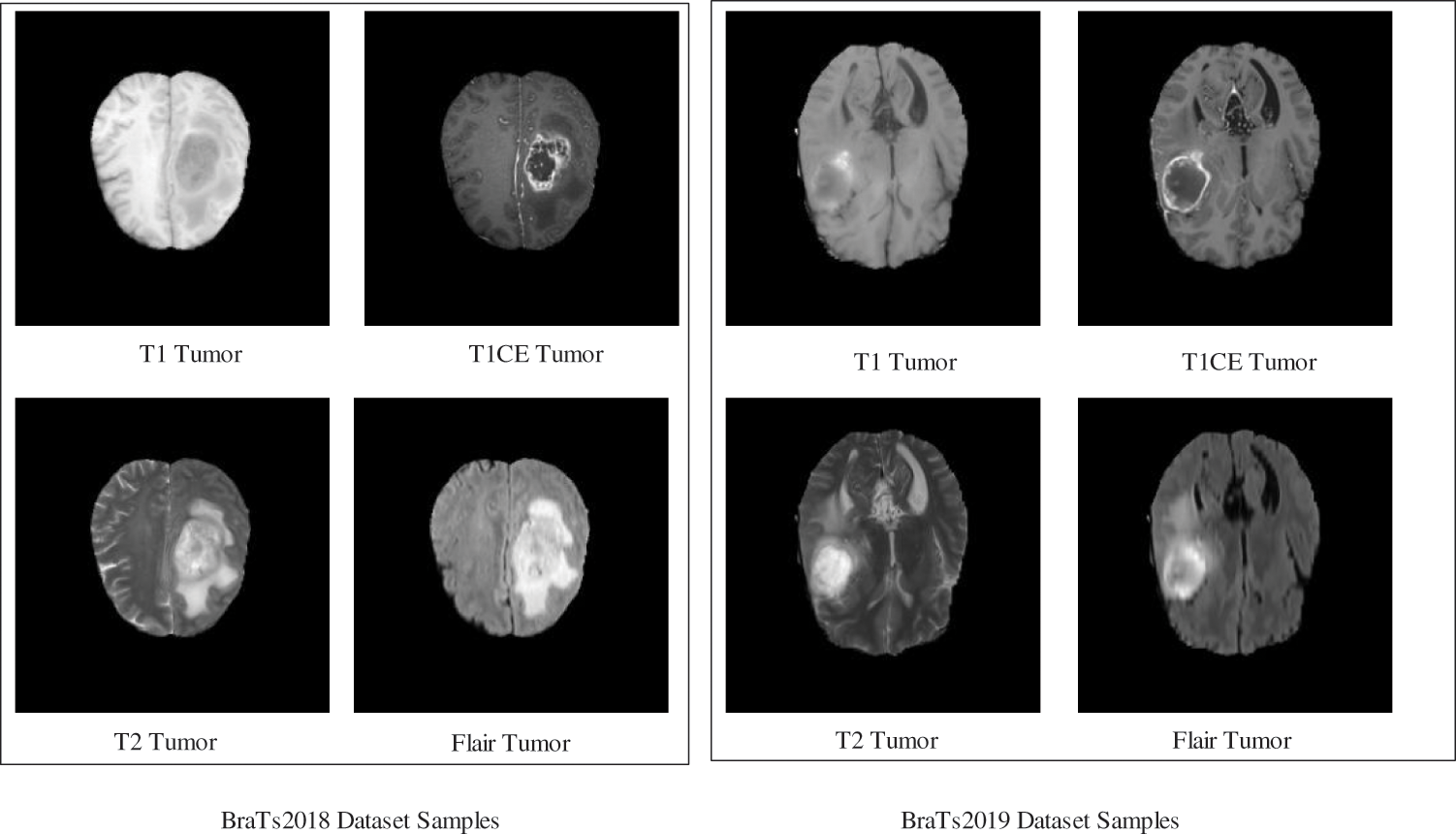
Figure 2: Sample brain tumor images
BraTs2019 [32]: This dataset consists of 335 scans for training, and validation scans are the same as Brats2018. Four sequences-T1, T1CE, T2, and FLAIR tumors are contained for each volume. Similar to the BraTs2018 dataset, the ground truths are generated manually with the help of expert neuroradiologists. All the MRI scans of this dataset have a volume of
In this work, we utilized 48,000 MRI samples from the BraTs2018 dataset (12,000 in each class), whereas for BraTs2019, the total extracted samples tally 56,000 (14,000 in each class). Initially, the extracted MRI samples had a dimension of
Consider
where,
Here, the value of
Here, i represents the number of extracted channels, and
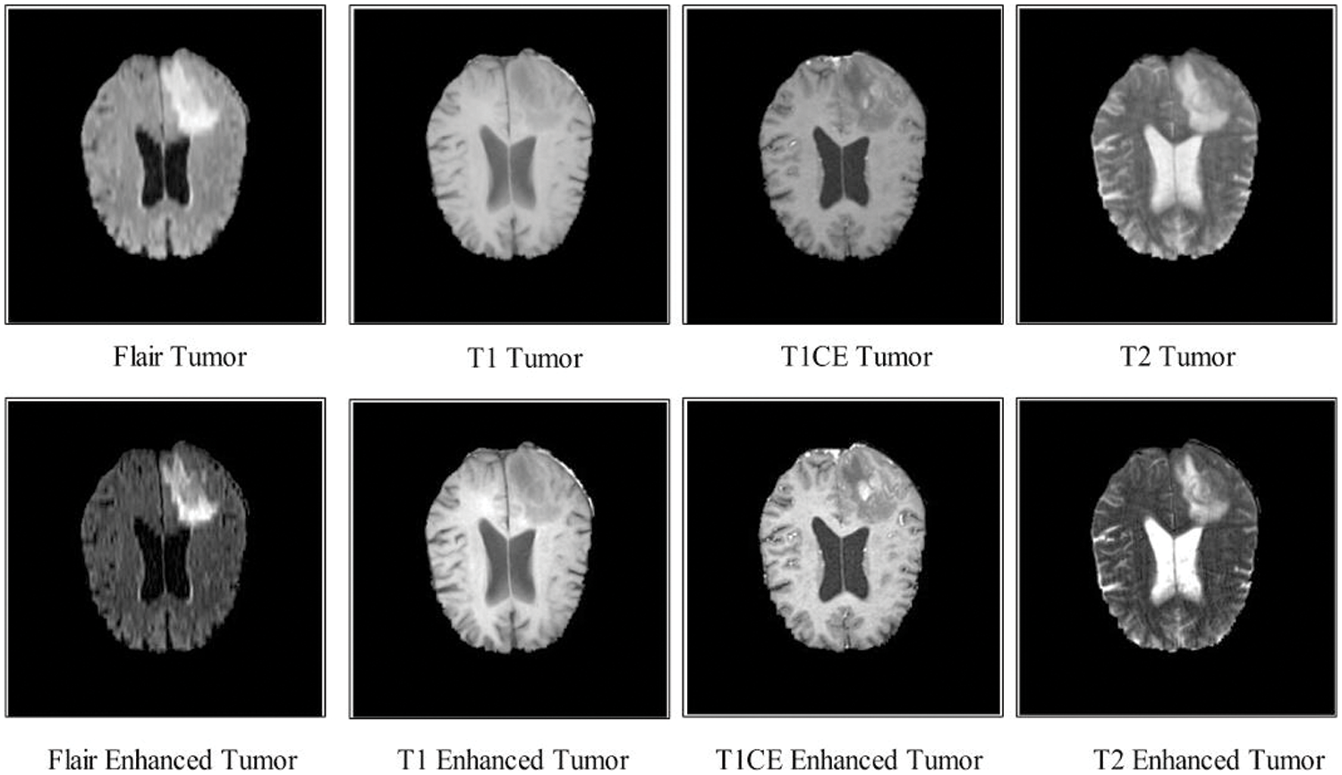
Figure 3: Enhanced MRI samples using a haze-CNN approach
Nasnet CNN architecture is a scalable network with building blocks optimized through reinforcement learning. Each building block consists of several layers (convolutional & pooling) and the recurrent time according to the network capacity. This network consists of 12 building blocks and a total of 913 layers. The total number of parameters is 5.3 million, less than the VGG and Alexnet [34]. In the fine-tuning process, the last classification layer is removed and added by a new FC layer. The main purpose of replacing this layer is that this network was previously trained on the Imagenet dataset, and the number of labels tallied at 1000. However, the selected datasets BraTs2018 and BraTs2019 include four classes; therefore, it is essential to modify this deep network.
After fine-tuning, deep transfer learning is employed to train this model; the TL’s main purpose is to reuse a pre-trained model for another task with less time and memory. Moreover, the TL is useful when the training data is fewer (target) than the source data.
Transfer learning: Given a source domain
In the training of the deep learning model, several hyperparameters are employed as specified–the learning rate is 0.0001, mini-batch size is 64, max epochs are 100, an optimization method is Adam, and the loss function is cross-entropy. The activation function for feature extraction is sigmoid. Visually, this process is shown in Fig. 4. This figure illustrates that the ImageNet dataset is used as source data for the pre-trained network. After fine-tuning, the model is trained on BraTs2018 and BraTs2019 datasets. As shown in Fig. 1, the fine-tuned NasNet-Mobile is trained separately on original and enhanced samples; therefore, two deep-learning models are obtained. On both trained models, features are extracted from the GAP layers and obtained a feature vector of dimensions
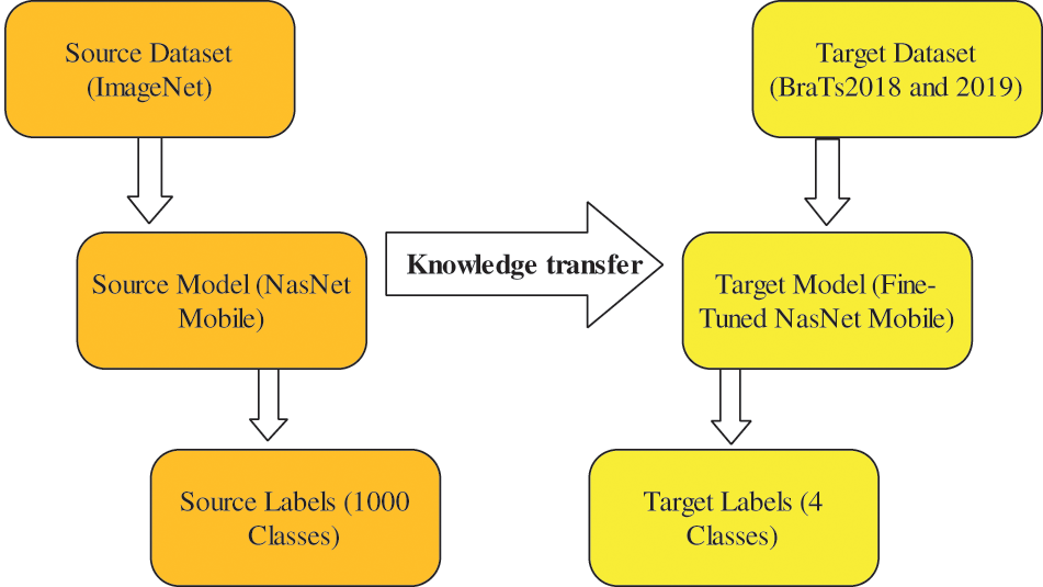
Figure 4: Features extraction using transfer learning
2.3 MCCA-Based Deep Features Fusion
Given
The
Based on this formula, both deep feature vectors are fused and obtain a new fused feature vector of dimension
2.4 Hybrid Feature Selection Algorithm
This work utilized a hybrid optimization algorithm for best feature selection. In the selection process, initially, a fused feature vector of dimension
The hybrid method is based on the enhanced WOA and Crow search algorithm (CSA). In addition, Mirjalili introduced a swarm intelligence algorithm known as WOA [35]. This algorithm is established on the predatory approach of humpback whales. Humpback whales catch a school of small fishes or krill close to the surface. This procedure generates specific bubbles with a ring path, and the operator is divided into three components. In the first phase of the algorithm, a prey is surrounded and attacked by a spiral bubble net (exploitation phase); in the second phase, whales randomly search for food (exploration phase). Mathematically, the WOA process is described as follows:
Encircling prey: Initially, the optimal position is not recognized; therefore, it is supposed that the current optimal solution is the objective prey or near to the optimal solution. After defining the best search space, the other search spaces try to set their location regarding the best search space.
where h denotes the current iteration,
Bubble-net attacking: The local search process is described as each humpback whale relocates to get near a prey within a dense ring while following a spiral-shaped path. Then, following the compact ring or spiral mechanism, a probability of 0.5 is set to renew the location of the humpback whale. The mathematical formula is defined as follows:
where
Searching for prey: The location of the current humpback whale is revised based on the random walk approach, defined as follows:
Based on the entropy value, the threshold function is defined to enhance the selection performance of the whale optimization algorithm, and it is defined as follows:
The best-selected features are passed to the Crow search algorithm to reduce some redundant features. This metaheuristic’s purpose is for a given crow i to be able to follow another crow j to identify its concealed food location. Therefore, it is important that the crow i position is constantly updated during this process. Furthermore, when food is stolen, crow i must move it to a new location. Accordingly, based on a swarm of crows (N), a CSA algorithm begins by initializing two metrics.
Location matrix: All the possible solutions for the problem in this study are represented by the location of crow e in the search space. The crow’s position at iteration
where N is the population size, d is the problem’s dimension,
Memory matrix: this matrix represents the memory of crows to store the location where their food is kept. Crows have an exact recollection of where their food is hidden, and it is also believed to be the best position for that particular crow. Therefore, at each iteration, there are two scenarios of crows’ movement in the search space:
In the first scenario, crow g is completely unaware that crow e follows him. Consequently, this means that the next position of crow e in the direction of the crow g’s hidden food site is denoted as follows:
where
The second scenario occurs when crow g realizes it’s followed by crow e. Consequently, to fool crow e, crow g will move to an entirely random location in the search region. Randomness determines Crow
where
where
Two publically available datasets, such as BraTS2018 [31] and BraTs2019 [32], are employed for the experimental process. In the validation process, 50 percent of the dataset images are utilized for the training, and the remaining 50 percent are utilized to test the proposed deep learning framework. In the deep learning model training, several hyperparameters are employed: learning rate is 0.0001, mini-batch size is 64, max epochs are 100, an optimization method is Adam, the loss function is cross-entropy, and the activation function for feature extraction is sigmoid. Furthermore, five different classifiers, such as multiclass support vector machine (MCSVM), weighted K-nearest neighbor (WKNN), Gaussian Naïve Bayes (GNB), ensemble baggage tree (EBT), and extreme learning machine (ELM), have been implemented for the classification performance. Finally, the testing results are computed through 10-fold cross-validation. The entire framework is implemented on MATLAB2021b using a desktop PC with 16 GB of RAM, 256 SSD, and a 16 GB graphics card.
Experimental process: The proposed deep learning framework is validated through several experiments: i) deep learning feature extraction from an average pooling layer of a fine-tuned NasNet-Mobile CNN trained on original dataset images and performed classification; ii) deep learning feature extraction from an average pooling layer of a fine-tuned NasNet-Mobile CNN trained on enhanced MRI images and performed classification; iii) fused deep features of both fine-tuned CNN models using the MCCA approach; and iv) the proposed hybrid feature optimization algorithm is applied on fused feature vector and obtains the best feature for final classification.
Results of BraTs2018 dataset: Table 2 presents the classification results for the middle steps of the proposed deep learning framework. This table calculates the results for NasNet-Org, NasNet-Enh, and fusion. NasNet-Org represents deep learning extracted features through NasNet-Mobile original sample images of the selected dataset, while NasNet-Enh represents feature extraction using enhanced MRI images. The ELM classifier gives better results, with 88.9%, 90.6%, and 91.8% accuracy than the other classifiers. According to the results given in this table, it is shown that classification performance is improved for the enhanced images that are further boosted after the fusion of both deep feature vectors. The computational time is also mentioned in this table, and it is observed that the time of NasNet-Enh and fusion steps is increased more than NasNet-Org. To resolve the challenge of high computational time and improve the classification accuracy, a hybrid feature optimization algorithm is applied to the fused feature vector, with the results presented in Table 3. The ELM classifier achieved the best accuracy of 94.8 percent, whereas the sensitivity rate was 94.62 percent. The computational time of ELM is 13.660 (sec), which was previously 66.3264 (sec) for NasNet-Org.


Fig. 5 illustrates the confusion matrix of the ELM classifier after the best feature selection. In this figure, it is noted that each tumor class prediction rate is above 90 percent. A time-based comparison among each middle step is also conducted, as plotted in Fig. 6. This figure describes that the fusion process consumed more time than the rest.
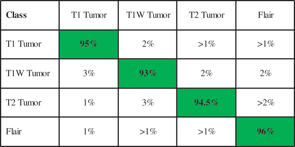
Figure 5: Confusion matrix of ELM classifier for BraTs2018 dataset
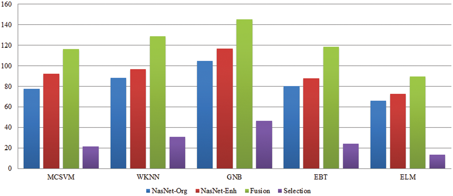
Figure 6: Time-based comparison of each middle step on selected classifiers using the BraTs2018 dataset
Results of BraTs2019 dataset: Table 4 presents the classification results for the middle steps of the proposed deep learning framework using the BraTs2019 dataset. The results given in this table are computed for NasNet-Org, NasNet-Enh, and deep features fusion. ELM classifier gives better results for the first three middle steps than the other classifiers, achieving accuracies of 88.0%, 89.3%, and 90.6%. According to the results given in this table, it is shown that classification performance is improved for the enhanced images that are further boosted after the fusion features. The computational time of each step for all classifiers is also mentioned in this table, while it is observed that the time of NasNet-Enh and fusion steps is increased more than NasNet-Org. This challenge is resolved through a hybrid feature optimization algorithm applied to the fused feature vector, with the results presented in Table 5. The ELM classifier achieved the best accuracy of 94.8 percent, whereas the sensitivity rate was 94.62 percent. These values showed that the selection of the best features not only reduced the computational time but also increased classification accuracy. The computational time of ELM is 23.100 (sec) after the feature selection process. The previous minimum time was 77.3484 (sec) for NasNet-Org features.


Fig. 7 illustrates the confusion matrix of the ELM classifier after the best feature selection. Time-based comparison among each middle step is also conducted, as plotted in Fig. 8. The time plotted in this figure shows the importance of the feature selection step. This figure also describes that the fusion of a deep learning process consumes more time than the other steps, such as NasNet-Org and NasNet-Enh.
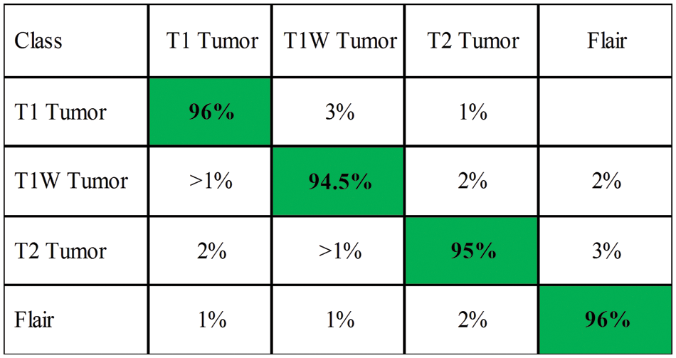
Figure 7: Confusion matrix of elm for BraTs2019 dataset

Figure 8: Time-based comparison of each middle step of the selected classifiers using the BraTs2019 dataset
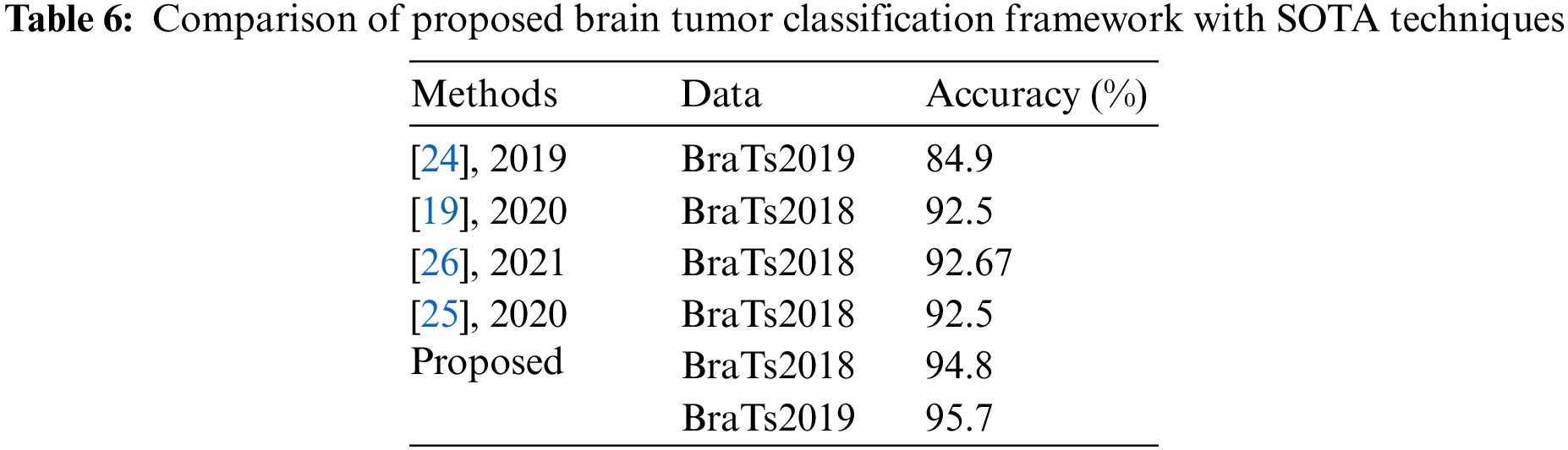
In Figs. 9 and 10, a comparison of middle stages is also performed and plotted. The precision is improved following the fusion procedure, as shown in these figures. The fusion accuracy is further tuned while the optimization approach enhances each classifier’s accuracy by over 4%. Furthermore, the computational time shown in Tables 2–5 indicates that the fusion process consumes more time than that saved by the proposed hybrid feature selection technique. Finally, the correctness of the proposed framework is compared to several previous approaches, as given in Table 6. Khan et al. [19] obtained an accuracy of 92.5 percent using the BraTs2018 dataset. Rehman et al. [26] used the BraTs2018 dataset and achieved an accuracy of 92.67 percent. Sharif et al. [25] presented a deep learning model and achieved an accuracy of 92.5% using the BraTs2018 dataset. In this article, the proposed framework obtained an accuracy of 94.8 percent on the BraTs2018 dataset and 95.7 percent on the BraTs2019 dataset. Overall, the proposed accuracy is improved as opposed to the existing techniques [19,25,26].
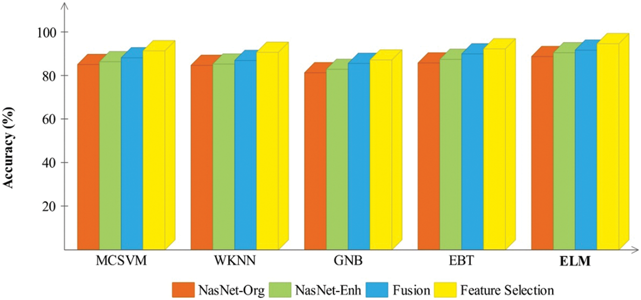
Figure 9: Comparison of each middle step of the proposed framework based on the accuracy for the BraTs2018 dataset
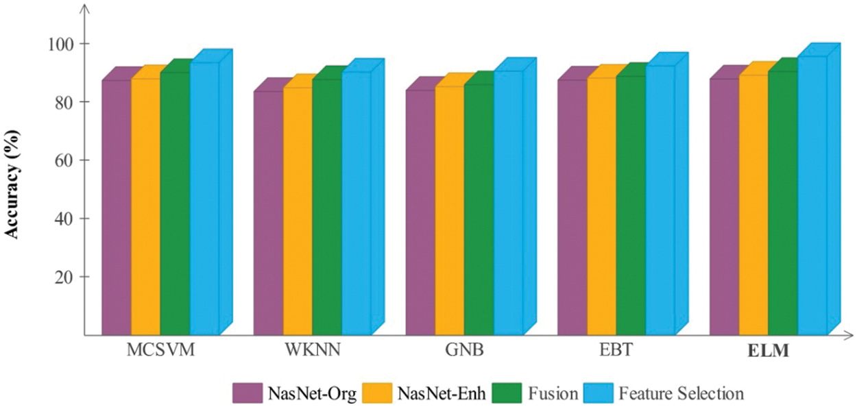
Figure 10: Comparison of each middle step of the proposed framework based on the accuracy for the BraTs2019 dataset
This research proposes a multimodal brain tumor classification framework based on two-way deep learning and hybrid feature optimization algorithms. The framework’s first stage was to train a fine-tuned two-way deep learning model on original and augmented images, which were then trained using TL. A multiset CCA-based system is employed to extract and fuse the features of the average pooling layers. Before being classified using an ELM classifier, the fused feature vector is enhanced using a hybrid HWOA-CSA feature optimization approach. The experiment used two publicly available datasets called BraTs2018 and BraTs2019, with 94.8 and 95.7 percent accuracy rates, respectively. In terms of accuracy, the proposed strategy outperforms recent SOTA techniques. According to the data, combining two-way CNN features improves classification accuracy. However, it increases the time consumed, but the proposed hybrid feature optimization approach overcame the long processing time. Tumor segmentation and CNN model training will be done in the future. In addition, the BraTs2020 dataset will be used in the testing process.
Acknowledgement: The authors extend their appreciation to the Deanship of Scientific Research at King Khalid University for funding this work through large group Research Project.
Funding Statement: This work was supported by “Human Resources Program in Energy Technology” of the Korea Institute of Energy Technology Evaluation and Planning (KETEP), Granted Financial Resources from the Ministry of Trade, Industry & Energy, Republic of Korea (No. 20204010600090). The authors extend their appreciation to the Deanship of Scientific Research at King Khalid University for funding this work through large group research project under Grant Number RGP.2/139/44.
Author Contributions: Conceptualization, Methodology, Software, Original Writing Draft: Muhammad Attique Khan, Reham R. Mostafa, Yu-Dong Zhang, and Jamel Baili; Validation, Formal Analysis, Visualization, Project Adminstration: Majed Alhaisoni, Usman Tariq, Junaid Ali Khan; Data Curation, Supervision, Funding, Resources: Ye Jin Kim and Jaehyuk Cha.
Availability of Data and Materials: Datasets used in this work are publicly available for the research purpose.
Conflicts of Interest: The authors declare that they have no conflicts of interest to report regarding the present study.
References
1. A. J. Tybjerg, S. Friis, K. Brown and B. Køster, “Updated fraction of cancer attributable to lifestyle and environmental factors in Denmark in 2018,” Scientific Reports, vol. 12, no. 5, pp. 1–11, 2022. [Google Scholar]
2. R. L. Siegel, K. D. Miller and A. Jemal, “Cancer statistics, 2015,” CA: A Cancer Journal for Clinicians, vol. 65, pp. 5–29, 2015. [Google Scholar] [PubMed]
3. D. N. Louis, A. Perry, G. Reifenberger and W. K. Cavenee, “The 2016 world health organization classification of tumors of the central nervous system: A summary,” Acta Neuropathologica, vol. 131, no. 5, pp. 803–820, 2016. [Google Scholar] [PubMed]
4. T. A. Abir, J. A. Siraji, E. Ahmed and B. Khulna, “Analysis of a novel MRI based brain tumour classification using probabilistic neural network (PNN),” Science and Engineering, vol. 4, no. 2, pp. 65–79, 2018. [Google Scholar]
5. S. L. Asa, O. Mete, A. Perry and R. Y. Osamura, “Overview of the 2022 WHO classification of pituitary tumors,” Endocrine Pathology, vol. 2, no. 5, pp. 1–21, 2022. [Google Scholar]
6. Z. N. K. Swati, Q. Zhao, M. Kabir and S. Ahmed, “Content-based brain tumor retrieval for MR images using transfer learning,” IEEE Access, vol. 7, no. 5, pp. 17809–17822, 2019. [Google Scholar]
7. S. Pereira, R. Meier, V. Alves and C. A. Silva, “Automatic brain tumor grading from MRI data using convolutional neural networks and quality assessment,” Understanding and Interpreting Machine Learning, vol. 2, no. 5, pp. 106–114, 2018. [Google Scholar]
8. B. Badjie and E. D. Ülker, “A deep transfer learning based architecture for brain tumor classification using MR images,” Information Technology and Control, vol. 51, no. 3, pp. 332–344, 2022. [Google Scholar]
9. V. Rajinikanth, S. Kadry and Y. Nam, “Convolutional-neural-network assisted segmentation and SVM classification of brain tumor in clinical MRI slices,” Information Technology and Control, vol. 50, no. 7, pp. 342–356, 2021. [Google Scholar]
10. S. Maqsood, R. Damaševičius and R. Maskeliūnas, “Multimodal brain tumor detection using deep neural network and multiclass SVM,” Medicina, vol. 58, no. 5, pp. 1090, 2022. [Google Scholar]
11. V. Rajinikanth, S. Kadry, R. Damaševičius and R. A. Sujitha, “Glioma/Glioblastoma detection in brain MRI using pre-trained deep-learning scheme,” in 2022 Third Int. Conf. on Intelligent Computing Instrumentation and Control Technologies (ICICICT), NY, USA, pp. 987–990, 2022. [Google Scholar]
12. T. M. Nguyen, N. Kim, D. H. Kim, H. L. Kim and S. J. Um, “Deep learning for human disease detection, subtype classification, and treatment response prediction using epigenomic data,” Biomedicines, vol. 9, no. 4, pp. 1733, 2021. [Google Scholar] [PubMed]
13. B. V. Isunuri and J. Kakarla, “Three-class brain tumor classification from magnetic resonance images using separable convolution based neural network,” Concurrency and Computation: Practice and Experience, vol. 34, no. 6, pp. e6541, 2022. [Google Scholar]
14. S. Deepak and P. Ameer, “Brain tumor classification using deep CNN features via transfer learning,” Computers in Biology and Medicine, vol. 111, no. 3, pp. 103345, 2019. [Google Scholar] [PubMed]
15. H. Mohsen, E. S. A. El-Dahshan, E. S. M. El-Horbaty and A. B. M. Salem, “Classification using deep learning neural networks for brain tumors,” Future Computing and Informatics Journal, vol. 3, no. 4, pp. 68–71, 2018. [Google Scholar]
16. M. I. Sharif, K. Aurangzeb and M. Raza, “A decision support system for multimodal brain tumor classification using deep learning,” Complex & Intelligent Systems, vol. 2, no. 1, pp. 1–14, 2021. [Google Scholar]
17. K. Kamnitsas, C. Ledig, V. F. Newcombe and D. K. Menon, “Efficient multi-scale 3D CNN with fully connected CRF for accurate brain lesion segmentation,” Medical Image Analysis, vol. 36, no. 2, pp. 61–78, 2017. [Google Scholar] [PubMed]
18. S. Alqazzaz, X. Sun, X. Yang and L. Nokes, “Automated brain tumor segmentation on multimodal MR image using SegNet,” Computational Visual Media, vol. 5, no. 1, pp. 209–219, 2019. [Google Scholar]
19. M. A. Khan, I. Ashraf, M. Alhaisoni and A. Rehman, “Multimodal brain tumor classification using deep learning and robust feature selection: A machine learning application for radiologists,” Diagnostics, vol. 10, no. 7, pp. 565, 2020. [Google Scholar] [PubMed]
20. S. Iqbal, M. U. Ghani Khan, T. Saba and A. Rehman, “Deep learning model integrating features and novel classifiers fusion for brain tumor segmentation,” Microscopy Research and Technique, vol. 82, pp. 1302–1315, 2019. [Google Scholar] [PubMed]
21. S. Ahuja, B. K. Panigrahi and T. K. Gandhi, “Enhanced performance of dark-nets for brain tumor classification and segmentation using colormap-based superpixel techniques,” Machine Learning with Applications, vol. 7, no. 5, pp. 100212, 2022. [Google Scholar]
22. A. K. Poyraz, S. Dogan, E. Akbal and T. Tuncer, “Automated brain disease classification using exemplar deep features,” Biomedical Signal Processing and Control, vol. 73, no. 14, pp. 103448, 2022. [Google Scholar]
23. V. Isunuri and J. Kakarla, “Three-class brain tumor classification from magnetic resonance images using separable convolution based neural network,” Concurrency and Computation: Practice and Experience, vol. 2, no. 4, pp. e6541, 2022. [Google Scholar]
24. Y. Xue, Y. Yang, F. G. Farhat and A. Barrett, “Brain tumor classification with tumor segmentations and a dual path residual convolutional neural network from MRI and pathology images,” in Int. MICCAI Brainlesion Workshop, NY, USA, pp. 360–367, 2019. [Google Scholar]
25. M. I. Sharif, J. P. Li, M. A. Khan and M. A. Saleem, “Active deep neural network features selection for segmentation and recognition of brain tumors using MRI images,” Pattern Recognition Letters, vol. 129, no. 4, pp. 181–189, 2020. [Google Scholar]
26. A. Rehman, M. A. Khan, T. Saba and N. Ayesha, “Microscopic brain tumor detection and classification using 3D CNN and feature selection architecture,” Microscopy Research and Technique, vol. 84, no. 2, pp. 133–149, 2021. [Google Scholar] [PubMed]
27. B. Ahmad, J. Sun, Q. You, V. Palade and Z. Mao, “Brain tumor classification using a combination of variational autoencoders and generative adversarial networks,” Biomedicines, vol. 10, no. 2, pp. 223, 2022. [Google Scholar] [PubMed]
28. J. Cheng, W. Huang, W. Yang and Z. Yun, “Enhanced performance of brain tumor classification via tumor region augmentation and partition,” PLoS One, vol. 10, no. 3, pp. e0140381, 2015. [Google Scholar] [PubMed]
29. C. Öksüz, O. Urhan and M. K. Güllü, “Brain tumor classification using the fused features extracted from expanded tumor region,” Biomedical Signal Processing and Control, vol. 72, no. 3, pp. 103356, 2022. [Google Scholar]
30. B. Erickson, Z. Akkus, J. Sedlar and P. Kofiatis, “Data from LGG-1p19qDeletion,” The Cancer Imaging Archive, vol. 76, no. 6, pp. 1–21, 2017. [Google Scholar]
31. L. Weninger, O. Rippel, S. Koppers and D. Merhof, “Segmentation of brain tumors and patient survival prediction: Methods for the brats 2018 challenge,” in Int. MICCAI Brainlesion Workshop, NY, USA, pp. 3–12, 2018. [Google Scholar]
32. Z. Jiang, C. Ding, M. Liu and D. Tao, “Two-stage cascaded u-net: 1st place solution to brats challenge 2019 segmentation task,” in Int. MICCAI Brainlesion Workshop, NY, USA, pp. 231–241, 2019. [Google Scholar]
33. K. Zhang, W. Zuo, Y. Chen and L. Zhang, “Beyond a Gaussian denoiser: Residual learning of deep cnn for image denoising,” IEEE Transactions on Image Processing, vol. 26, no. 3, pp. 3142–3155, 2017. [Google Scholar] [PubMed]
34. B. Zoph, V. Vasudevan, J. Shlens and Q. V. Le, “Learning transferable architectures for scalable image recognition,” in Proc. of the IEEE Conf. on Computer Vision and Pattern Recognition, NY, USA, pp. 8697–8710, 2018. [Google Scholar]
35. Q. V. Pham, S. Mirjalili, N. Kumar and W. J. Hwang, “Whale optimization algorithm with applications to resource allocation in wireless networks,” IEEE Transactions on Vehicular Technology, vol. 69, no. 14, pp. 4285–4297, 2020. [Google Scholar]
Cite This Article
 Copyright © 2023 The Author(s). Published by Tech Science Press.
This work is licensed under a Creative Commons Attribution 4.0 International License , which permits unrestricted use, distribution, and reproduction in any medium, provided the original work is properly cited.
 Downloads
 Citation Tools