Deep Learning-Based Model for Detection of Brinjal Weed in the Era of Precision Agriculture

1  Introduction

According to research statistics from the Food and Agriculture Organization Corporate Statistical (FAOSTAT) Database [1], India is the second-largest producer of brinjal in the world after China. In 2022, India produced over 12.98 million metric tons of brinjal crop across the nation [2,3], which signifies the importance and popularity of the crop. It is a vegetable crop grown all over India except in higher-altitude areas [4]. In many developing countries like India (as per the World Bank), as shown in Fig. 1a, the GDP contribution of agriculture, forestry, and fishing is decreasing due to the high and fast growth rates of services in the industries sector [5,6]. In addition to the fact that India’s agriculture sector is crucial to the country’s economy, it also faces a few challenges like unpredictable climate, poor supply chain, and low productivity [7–9]. India today has almost 315 million rural population using smartphones and the Internet. Technology brought improvisations to irrigation systems, crop management, and equipment harvesting tools, predicting the ideal weather for sowing and harvesting. As shown in Fig. 1b, India positions itself as second in the production of brinjal [10,11] across the globe. As shown in Fig. 1c, brinjal is India’s third most vegetation filled.

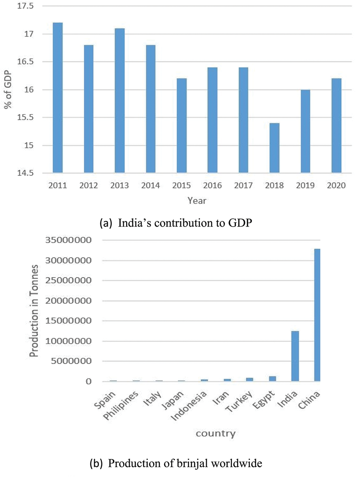
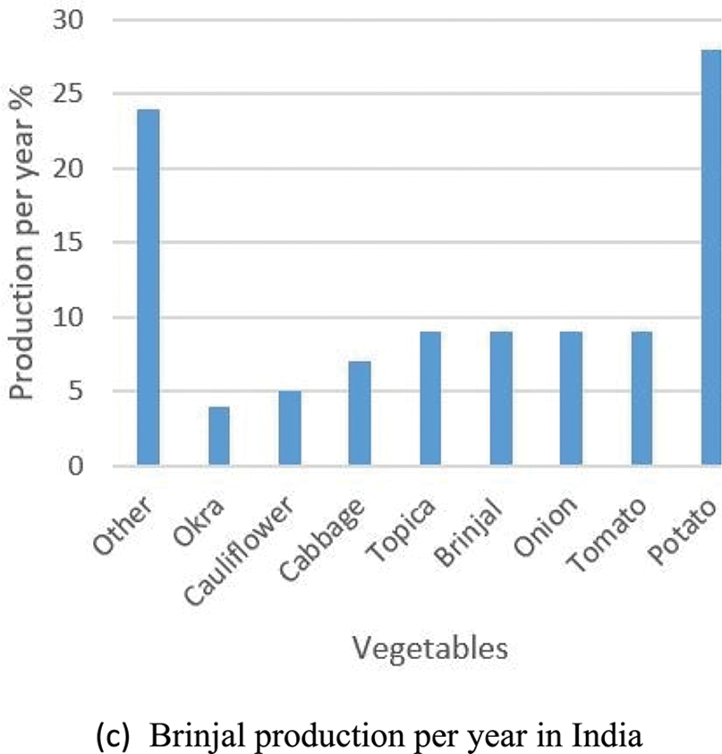
Figure 1: Statistic for the need for weed detection

Given the importance of the brinjal crop in the economic context, it is necessary to use techniques that maximize its productivity and yield quality. To enhance the productivity of the vegetable crop, various factors such as proper water and nutrition for the crop should be considered as control over weeds [12,13]. Therefore, it is crucial to reduce the losses imposed by weeds. According to estimates, Fig. 2a illustrates how crops typically lose 20–80 percent of their productivity to weeds, diseases, and pests. Herbicide application is a standard solution to avoid weeds in vegetable crops, including brinjal [14,15]. Statistics shown in Fig. 2b reflect that agricultural tech startups have raised over 800 million USD in the last six years across the globe [10].

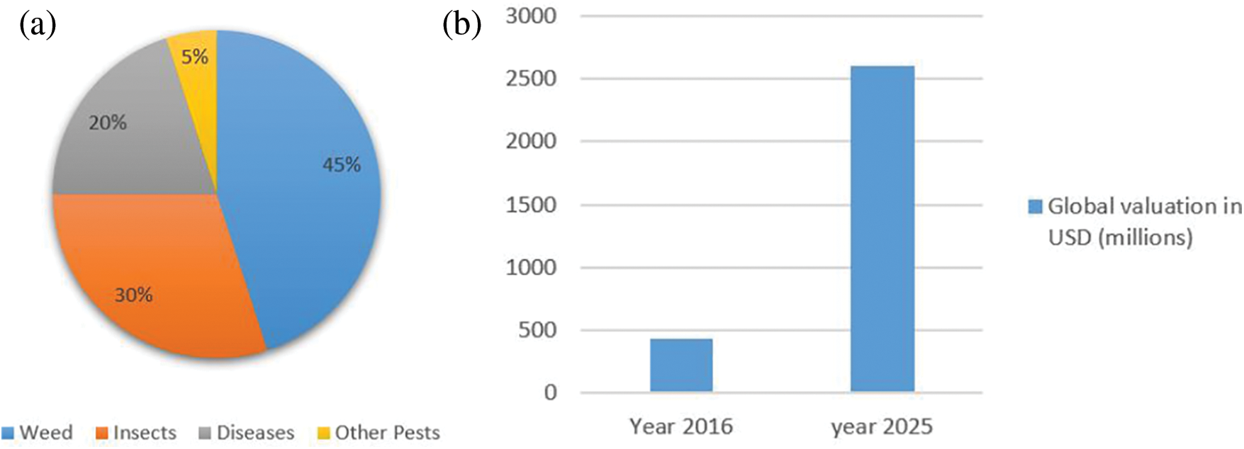
Figure 2: (a) Losses due to weed (b) AI techniques in smart agriculture

Crops treated with chemical application lead to a number of health, environmental, and biological issues [16]. Moreover, the high costs of herbicides and their adverse effects on human health are also a few concerns [17]. The excessive usage of herbicides can make the weeds resist the chemicals. Few studies have shown that a common herbicide (Glyphosate) has toxic elements that are harmful to human beings [18–20]. This must be considered part of the technological revolution and treated as a priority issue. Therefore, Artificial Intelligence (AI) can contribute to the issue by efficiently delivering solutions that cater to the purpose. Continuous research is underway to control weeds using biological methods like deploying natural microbes or insects that rely on and feed upon weeds [21], reducing negative impacts on herbicide chemicals. Growing technology in PA follows the practice of site-specific weed management (SSWM) [22–24]. Developing computer vision and Deep Learning (DL) technologies would simplify the object detection task. These technologies are extensively studied to identify weeds [25,26]. Conventional techniques such as image preprocessing, feature extraction, classification, and segmentation are explored for weed detection [27,28]. It works well when images are captured under perfect conditions and at specific plant growth stages [23,29]. Hence, the potential of DL has been utilized in PA, especially for weed detection [30,31]. Compared to conventional techniques discussed above, DL can learn the hidden feature expression and hierarchical insights from the images, which helps avoid the tedious process of extracting and optimizing the hand-crafted features [32]. Furthermore, semantic segmentation is one of the most effective approaches for alleviating the effect of occlusion and overlapping since pixel-wise segmentation can be achieved [33]. The main objective of this paper is to do the classification of images and object detection of weeds from the crop images of brinjal, which can further need to estimate the weed densities for successfully achieving SSWM for herbicide application expending a few segmentation models, such as Convolutional Neural Network (CNN), U-Net, LinkNet, and SegNet.

1.1 Research Contributions

Following are the research contributions of the proposed work:

•   We generated a real-time dataset by collecting images of brinjal crop variants from a farm field of brinjal vegetable crops near one village named Kudasan, Gandhinagar, Gujarat, India.

•   We utilized a DL-based model for weed identification from brinjal crop fields. Implementation of the proposed model, including object classification and object detection, is performed using CNN and DL Models (ResNet18, YOLOv3, CenterNet, Faster RCNN).

•   The performance of the proposed model is evaluated on Intersection over Union (IoU) and memory usage along with various standard metrics such as F1-score, precision, and recall.

1.2 Novelty

The classification and object detection of weeds has been the subject of substantial agricultural research. Despite brinjal being the most widely grown plant in the world, weeds have only ever been researched for potatoes and soybeans. The leaf images of weeds like Acalypha Indica and Amaranthus Viridis are similar to those of brinjal leaves, making it difficult to train an accurate model. According to a study, deep pre-trained models followed by classification can give effective identification outcomes.

1.3 Organization of the Paper

The rest of the paper is organized as follows. First, Section 2 covers the literature review with a relative comparison of the DL-based model to detect brinjal weed. Next, Section 3 addresses the proposed model, and Section 4 shows the results analysis and discussion of the proposed model. Finally, the paper is concluded in Section 5.

2  Literature Review

This section describes related work on weed detection using various methodologies (as shown in Fig. 3). We have considered the research articles published in the past ten years on a variety of crop and vegetable datasets, applications, and methodology for weed detection studied to satisfy the following objectives:

Figure 3: Task flow for literature survey carried out in the proposed work

1. Herbicide-Use Optimization-saves farmers’ money on herbicides and aids organic farming.

2. Effective Site-Specific Weed Management-Only spraying herbicides to parts of plants affected by weed instead of spraying their entire fields with herbicide.

3. Reduce manual intervention and decrease laborious process: Hand weeding is tedious and time-consuming.

4. For cost-effectiveness in farm labor expenses, labor shortages have increased the cost of hand weeding.

5. Utilize the potential of PA-Technologies such as DL has been helpful in these tasks.

6. Improve the output metrics by the proposed architecture of the model-Different researchers have applied various methods to help accomplish the task.

Fig. 3 shows the task flow for the literature survey in the proposed work, which helped identify the correct reference research more aligned with the proposed study. For example, Wang et al. [34] developed a real-time embedded device for weed detection using sensors, a control module, and a global-positioning system using classification algorithms. The system was tested in two wheat fields [35], where the classification part was majorly dependent on the sensors, which could not perform well when the positions of the sensors were changed. Late on, Torres-Sospedra et al. [36] applied two stages procedure on smooth ensembles of the neural networks for weed detection in orange groves. In the first stage, the main features of an image, like trees, trunk, soil, and sky, are determined, and in the second stage, weeds are detected from those areas, which are determined to be the soil in the first stage. Algorithms used for color detection are not used in the diversified environment, and even the dataset size was very small (10 training and 130 tests). Hameed et al. [37] extended research towards detecting weed, wheat, and barren land in a wheat crop field using background subtraction and image classification. The dataset was self-developed using a drone with 4000 × 3000 pixels resolution in a format of JPEG. The classification part is carried out using computer vision and image processing techniques. The results achieved (99%) are good enough, but it is only reasonable to detect weeds, barren land, and wheat. Weed detection involves crop and weed shape, size, and color techniques.

Dos Santos Ferreira et al. [38] have shown the performance of detection in soybean crops to classify among grasses and broadleaf using CNN and Support Vector Machines. In contrast, Bakhshipour et al. [4] applied weed detection in sugar beet crops with four types of weed Principal Component Analysis (PCA) and Artificial Neural Networks (ANN). Furthermore, Bakhshipour et al. [39] identified weeds from sugar beets with shape features ANN and Support Vector Machine (SVM) with comparative analytics for shape features, including other features on DL models. Asad et al. [8] applied semantic segmentation on the canola field for weed detection using U-Net and SegNet models for segmentation. Ashraf et al. [40] classified the rice crop images based on their weed density classes, such as no, low and high weeds using SVM and Random Forest. Duncan et al. [41] used object-wise semantic segmentation of images into the crop, soil, and weed. The encoder decoder network model was applied to achieve a mean IoU of 9.6. Raja et al. [33] achieved higher accuracy in weed detection in Unmanned Aerial System (UAS) imagery by field robot and Unmanned Aerial Vehicle (UAV) with the use of deep learning architectures U-Net, SegNet Fully Convolution Network (FCN), and DepLabV3+. Subeesh et al. [42] found the bell papers crop and weed identification with effective model Deep CNN models AlexNet, GoogLeNet, Inception V3, and Xception Inception V3 with an accuracy of 97.7%. Researchers worked on these techniques; for example, Perez-Ortiz et al. [43] worked on a semi-supervised system for mapping weeds in sunflower crops. However, the framework highly focuses on the row plant images taken from a distance. In contrast, our dataset is at the plant level and zoomed to plant leaves and weeds. Then, Partel et al. [44] developed a low-cost technology for precision weed management, which aligns with our objective of effective herbicide application. Still, after classifying the plants and weeds using DL algorithms, the research lacks comparison with the traditional broadcast sprayers that are usually employed to treat the entire field to control the pest. Various researchers also use graph-based DL methods for weed detection. For example, Hu et al. [45] developed a convolutional graph network to identify multiple types of weeds from RGB (Red, Green, and Blue) images taken in complex environments with multiple overlapping weed and plant species in highly variable lighting conditions. Classification (here recognition) is done using the ResNet-50 backbone and the DenseNet-202 backbone with five cross-fold-validation, and the Res-Net50 backbone achieved state-of-the-art performance as Graph Weeds Nets. The limitation of this research is that it is done for many different types of weeds and does not explicitly target any vegetation, crop, or plant. Though, the main essence of the paper achieved is the use of convolutional networks for better classification. Along with the latest DL technologies used for image datasets, some researchers show the use of various image descriptors for feature extraction.

Prolonging the research, Bosilj et al. [46] emphasized pixel-based crop vs. weed classification methodologies, particularly in challenging circumstances with overlapping plants and illumination variation. The study compares the benefits of content-driven morphology-based descriptors and multiscale profiles to state-of-the-art feature descriptors with a fixed neighborhood, such as histograms of gradients and native binary patterns previously used in PA. The study used two datasets, the first of which is the Sugar Beets dataset 2016 (280 images), and the second is the Carrots dataset 2017. Classification is done using a Random Forest Classifier. More extensive AP descriptors based on numerous hierarchies are among the drawbacks. Nevertheless, it can potentially improve pixel-based classification and make it more accurate. Furthermore, combining region-based classification and morphological segmentation with hierarchical image representation could improve by adding the benefit of reusing the hierarchical picture representation.

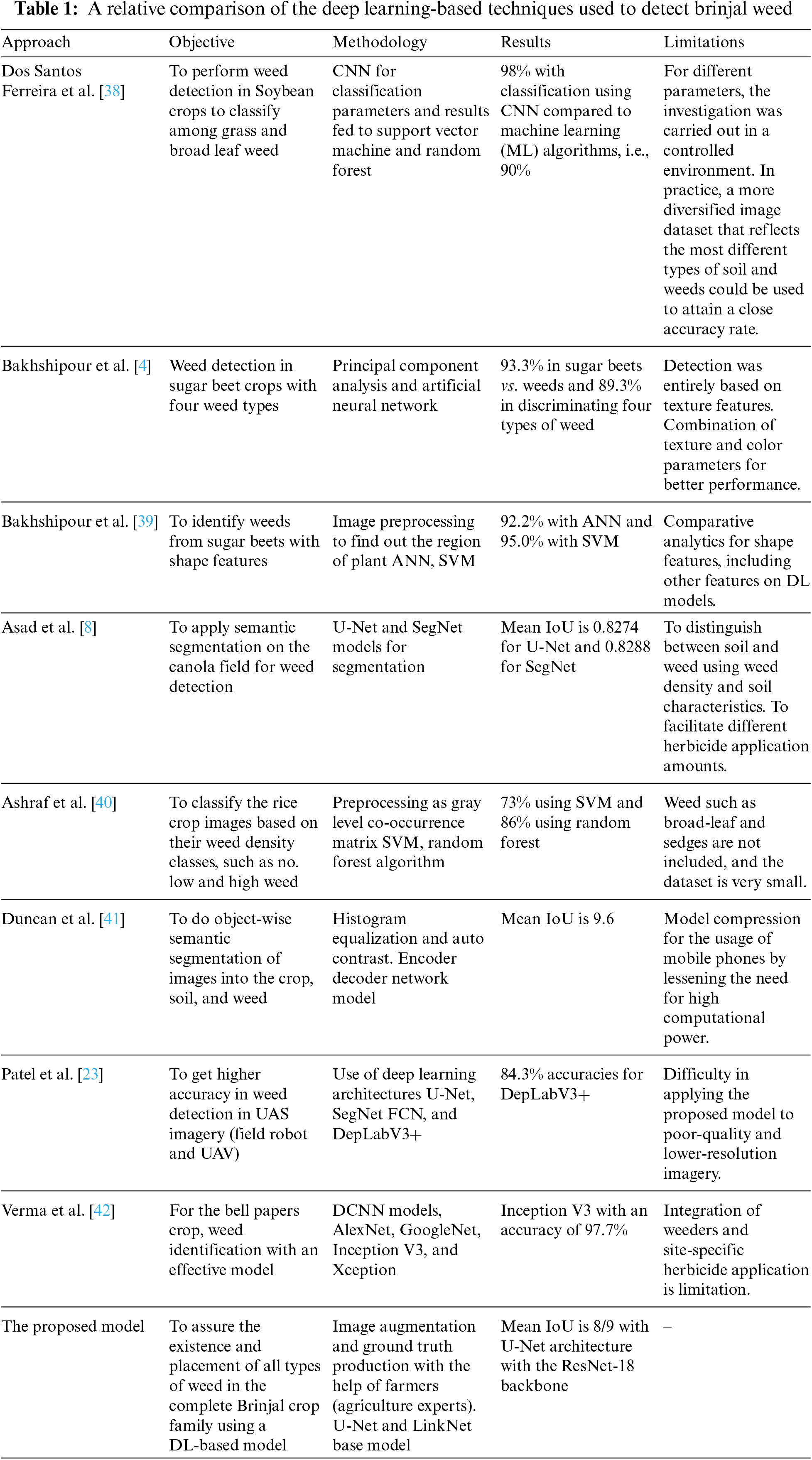
The most potent computational phase is segmentation, for both segmentation and feature extraction. Bell papers weed identification by four DCNN models, Inception V3, AlexNet, GoogLeNet, and Xception, were used in specific agricultural application research by Verma et al. [42], where the Inception V3 model is a better fit for higher accuracy. For future development, weeders and site-specific weed management modules could be combined. The dataset is manually collected from ICAR-Central Institute of Agricultural Engineering Bhopal, India. Raja et al. [33] created a more powerful architecture using data from the Sugar Cane Orthomosaic and Crop/Weed Field Image Dataset. To improve weed for recognition accuracy in UAS imagery (field robot and Unmanned Aerial Vehicle (UAV)), a model is created using deep learning architectures U-Net, FCN, SegNet, and DepLabV3+, with DeplabV3+ receiving 84.3% accuracies. For low-quality, low-resolution imagery, the model is ineffective. Table 1 compares the DL-based techniques used to detect brinjal weed concerning parameters such as objectives, methodology, results, and limitations.

3  The Proposed Model

In this section, the authors proposed a paradigm, provided a complete flow diagram displaying the links between modules, and described a comprehensive method. As per the architecture shown in Fig. 4, it comprises five modules: Dataset collection, Data preprocessing, Object detection, Deep Learning Models, and Evaluation metrics.

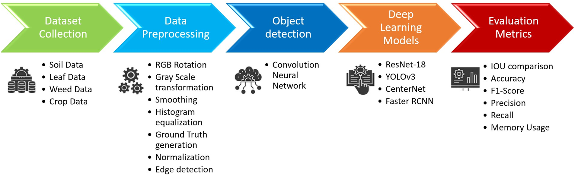
Figure 4: The proposed model

Captured crop images from a real-time environment need preprocessing to smooth images. It includes segmenting soil from the background, image augmentation, grayscale transformation, and Image resizing. Attributes, such as shape, size, and color, are considered for the normalization and scaling of the images. Image preprocessing is responsible for furnishing the Image in the required form of the weed image dataset [47]. Dataset augmentation is used to increase the variety of the dataset. For the same, images are blurred, horizontally flipped, and rotated manually. Ground truth generation is an important step for any segmentation task. We give the label and the Image as weed and non-weed parts to the DL model. The need to generate ground truth by mapping and interpreting the regions of plant and non-plant from the Image as the dataset is collected manually. The final preprocessing phase is to rescale the Image from RGB to 250 × 250 pixels, included in the weed dataset. Preprocessed images are passed to the CNN model to extract features, as shown in Fig. 5. Feature extraction consists of the shapes and sizes of leaves and weeds. CNN is used for learning the primary shapes present in the first layer. It also adjusts itself to learn other shapes in the deeper layers, followed by DL models for enhanced accuracy. In the object detection method, the Image is identified pixel-by-pixel. YOLOv3, CenterNet, Faster RCNN, and ResNet18 models were used for training and testing the features extracted from CNN. The post-processing and evaluation metrics module discusses the trend of best metrics used for segmentation Intersection over Union (IoU) [48]. Each of the modules has been explained in detail in Section 4.

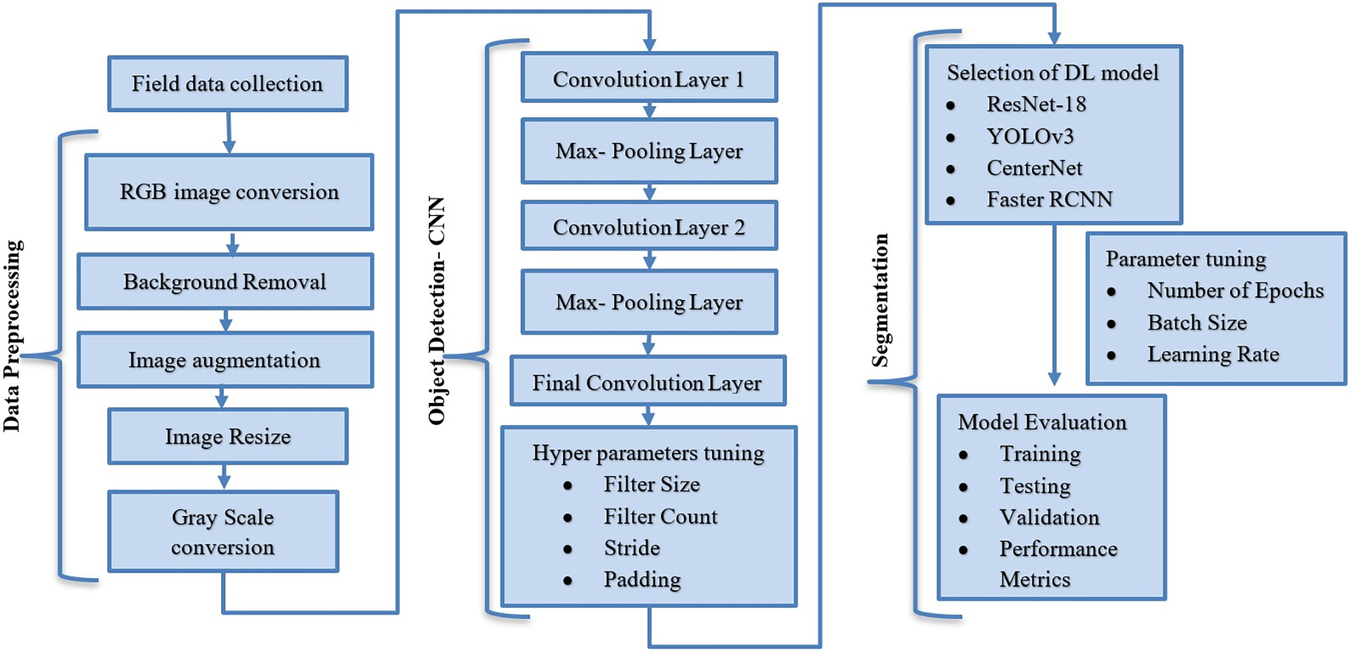
Figure 5: Flow diagram of the proposed model

3.1 Dataset Description

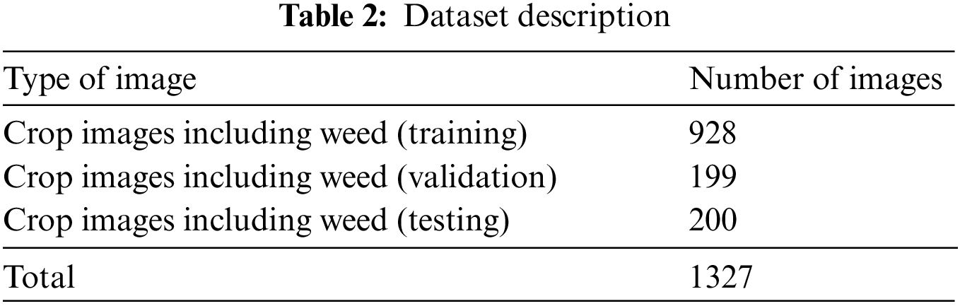
Dataset acquisition includes capturing a single image of weeds, leaves, and soil. The data used in the experiment is manually collected from a field farm of brinjal crops near one village named Kudasan, Gandhinagar, Gujarat, India. There were a few iterations of data capturing to ensure the perfect quality of the images of brinjal with weeds and different stages of crop growth. The images are in RGB (Red, Green, Blue) format. The ideal light, weather, weed, and plant growth conditions are matched for dataset collection. Proper level from the ground is also maintained for each image. In summary, 218 images were collected with augmentation from the field, and 1109 images were taken from dataset providers [49–51]. The dataset for the model’s training, validation, and testing is bifurcated as Table 2 from a total of 1327 images.

The image-capturing device had a 48 MP resolution of MI (Xiaomi). The captured image of the Brinjal crop is shown in Fig. 6a, and after the augmentation, the application is shown in Fig. 6b. The Brinjal crop dataset was made available as open-source [52]. After the images are fed to the architecture, the output identifies different objects present in the image, like soil, weed, crop leaves, crop flowers, and brinjal. The same is depicted in Fig. 7.

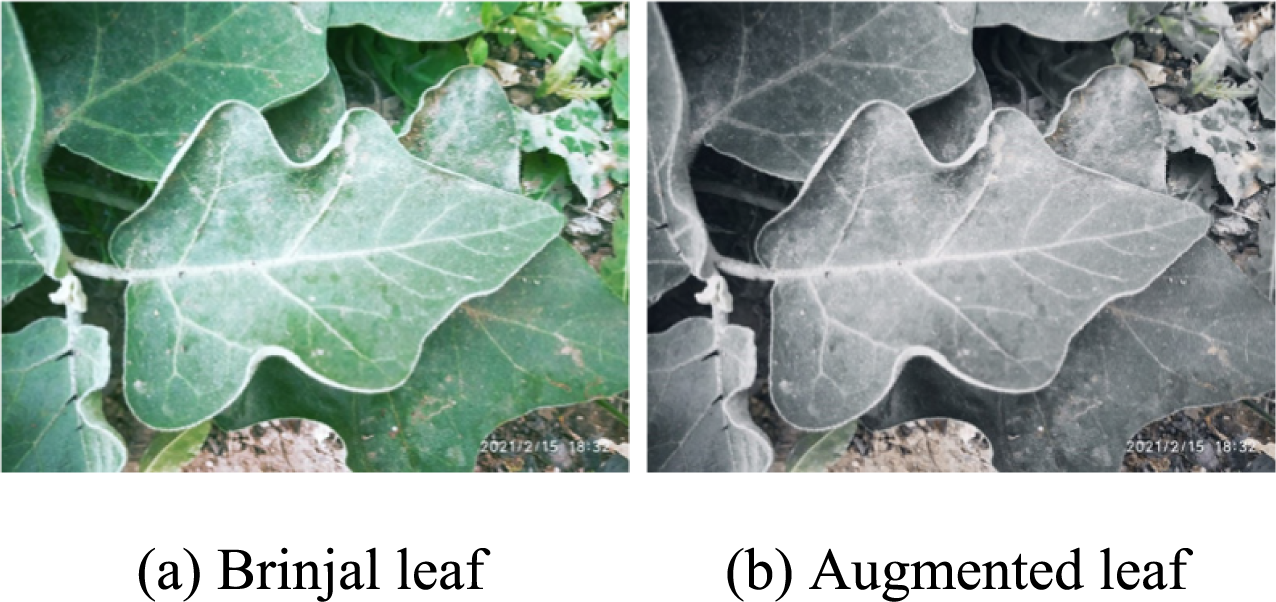
Figure 6: Captured images of the brinjal crop before and after augmentation using the proposed model

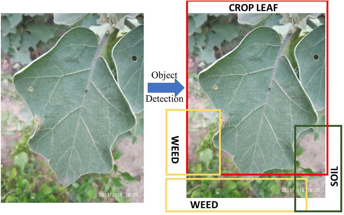
Figure 7: Object detection in weed classification using the proposed model

3.2 Ground Truth Generation

The input layer of the DL model needs ground truth creation since it generates labeled images. As the dataset is collected manually, there is a need to generate ground truth by mapping and annotating the regions of plant and non-plant from the image in Fig. 8. We are required to divide the images into sections carefully. This would lead to a binary segmentation problem in terms of DL. For instance, as shown in the below collection of images, there is a standard semantic segmentation process where input, ground truth & prediction are the main parts. Ground truth generation helps in pixel-wise classification for the segmentation model. The GNU Image Manipulation Program (GIMP) is an image editor system used for ground truth generation. It includes various choices for image manipulation and a toolkit for efficiently and precisely constructing the ground truth. To create ground truth, two colors are applied, and both of them resemble different parts of the image, including plants and non-plants. These portions are drawn with the help of the GIMP cursor tool and then colored using the same as shown in Fig. 8.

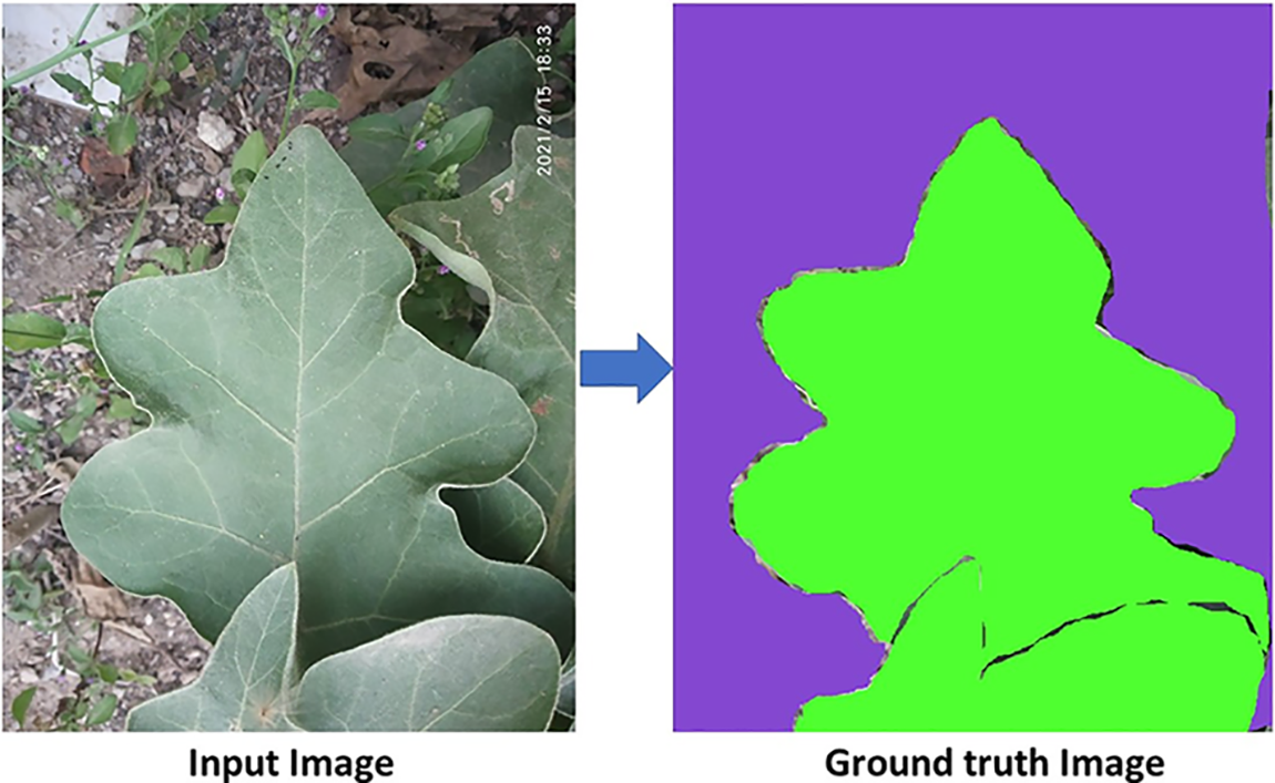
Figure 8: Ground truth generation

3.3 Data Pre-Processing Image Augmentation

The dataset consists of manually collected images with varied sizes and shapes that must be reformed into shapes similar to all the images [53]. For this research project, we have cropped and resized the dataset images from different sizes to 256 × 256, all while keeping the color channels intact [54]. Then, the images are passed from the normalization process by subtracting each channel’s mean from the original value and later dividing the channels’ standard deviation [55] for the learning phase, which will contribute in a better way to the segmentation model.

The data augmentation phase is a common process in DL-based projects to ensure sufficient data provision to the model for the learning phase [56]. The dataset’s diversity in terms of shape, size, location, and orientation of weed helps the model perform well. Many methods deal with adding more synthetic samples for text data augmentation by getting the nearest neighbor points. While working on the image projects, we can augment the data by using basic methods such as flipping the image vertically and horizontally and adding some noise [47]. We have augmented the data with random horizontal and vertical flips. This augmentation step aids in extending the amount of training dataset, and by including augmented samples created using the methods described above, the model’s learning experience is improved. It also increases the accuracy of the model’s measuring key performance indicators (KPIs) when the test or actual data is inputted into the trained model [25]. It also enables the model to learn previously missing features and strengthen connections in the network [16].

3.4 Object Classification

The CNN parameters employed in this model are described as follows. The first two-dimensional convolutional layer is performed with 448 parameters and 148 × 148 × 16 samples. With the pooling implementation, these samples were down-sampled to 74 × 74 × 16. Hence, out of the whole image, a particular section was focused on. Then, another convolutional layer of the same dimension is involved in deepening the section and extracting the features precisely. Further, 4640 parameters are recognized to deepen the model, and more features are extracted to enhance the precision and efficiency of the model. Likewise, another three layers are implemented, followed by pooling in each layer. The final number of parameters was 18496. These parameters flattened to convert the map of more dimensions into a single-dimension array. The experiment is carried out on an utterly connected layer, and 2-Dense layers append the connected layer to the neural network. A total of 9,494,561 parameters were taken for the proposed model.

3.5 Object Detection

Different object detection models have been tested based on the literature survey. YOLOv3, CenterNet, Faster RCNN, and ResNet18 have used different backbone architectures per this project’s dataset. We had RGB images and the binary segmentation classes with only two differentiated classes. As the dataset size is average, models have to be chosen accordingly. Researchers have used U-Net for canola and paddy field image segmentation tasks and achieved good results. U-Net is a type of CNN. The U-Net Model successfully delivers better results in pixel-to-pixel classification for biomedical images [57,58]. ResNet18 is a backbone for one of our beneficial and referred research papers, where several operations are used, including Convolution, Max-Pooling, Up-Sampling, and Transposed Convolution. The convolution operation takes two inputs: the input image and the set of filters or feature extractors [59]. The Convolution operation and the Max-Pooling operation effectively lead to image size reduction. It is selected because of its good performance in previous research records and relatively low computation cost [60].

Based on the literature review, many segmentation models have been tested. A CNN called YOLOv3 is used to identify objects in real-time [56]. Originally, Darknet had a 53 layers network trained on ImageNet [61]. But here, a variation of Darknet is being used. The primary components of the Darknet have skipped connections and 3 × 3 and 1 × 1 filters. This Darknet variant has 53 more layers, with 106 layers of the underlying convolutional architecture. YOLOv3 calculates the classification loss for each label using binary cross-entropy, and logistic regression is used to forecast object confidence and class predictions. It has three hyperparameters, class threshold, non-max suppression threshold, and input height and shape. This model has three output layers and finds objects by applying 1 × 1 detection kernels to three different-size feature maps at three distinct points across the network. The classification loss for each label is calculated using binary cross-entropy, and class predictions and object confidence are forecasted using logistic regression. The YOLOv3 has three output layers. The first layer contains the bounding box coordinates, classes, and confidence (1, 13, 13, 13), where 255 denotes. The second layer works at a different scale and divides your image into a grid of 26 × 26 squares. The third layer divides your image into a grid of 52 × 52 squares and predicts the bounding box coordinates for each grid cell [62,63].

CenterNet is an anchorless object detection architecture. This technique dramatically accelerates inference [57]. CenterNet recognizes each object as a triplet rather than a pair of key points. It uses two specifically created modules: center pooling and cascade corner pooling. It improves the data acquired by the top-left and bottom-right corners and provides more recognizable information in the center areas. Center pooling is used to predict center key points. This maximizes the response from a feature map’s central key point in the vertical and horizontal dimensions. Corners can extract features from center areas because of cascade corner pooling. It initially looks along a boundary value, then inside the box and where the maximum boundary value is placed to get a maximum internal value. Then, the sum of the two highest values is calculated. The output produced by CenterNet is [0,1] (WR × HR × C) where R = output stride and C = number of keypoint types. By default, we use output stride R = 4. A prediction of 1 corresponds to the detected keypoint, while 0 is background [22].

Another object identification architecture can be used as a Faster RCNN [64]. Convolution layers, Region Proposal Network, and Classes & Bounding boxes prediction comprise its three components. The filters are trained to extract the right picture characteristics in the convolution layers. A tiny neural network called the Region Proposal Network (RPN) slides on the final feature map created by the convolution layers and aids in determining whether or not there are objects present as well as their bounding boxes. With the regions recommended by the RPN as input, it now uses a fully connected neural network to forecast item class (classification) and bounding boxes (regression).

3.6 Evaluation Metrics

The evaluation metrics are chosen per the proposed model and the objective of this work. The dataset is divided into the train, validation, and test sets, each comprising 70%, 15%, and 15% of the total. This guarantees that the model’s universal performance is not limited to the training dataset. However, there is overfitting when the validation loss stops decreasing or increases while the training loss keeps going down. Here, we are doing semantic segmentation of weeds and plants; therefore, the efficiency parameters are different in the segmentation model. The evaluation measures for semantic segmentation include IoU, mean IoU, accuracy, recall, precision, F1-score, and memory usage [65]. True positive(TP) values for our dataset are images containing weed and are accurately detected. False positives(FP) are images without weed but identified as “weed.” False negatives (FN) are images having weed and detected as “no weed.” The efficiency parameters are defined as Eqs. (1)–(3) as follows:

1.    Accuracy: It is the proportion of right forecast perceptions to the complete number of perceptions. It holds significance when the information base is symmetric.

2.    Precision: It is the proportion of accurately anticipated positive perceptions to the all-out anticipated positive perceptions.

Precision=TPTP+FP(1)

3.    Recall: The proportion of right-judged positive perceptions to perceptions in it.

Recall=TPTP+FN(2)

4.    F1-score: It is a weighted average of Recall and Precision.

F1−score=2×Precision×RecallRecall+Precision(3)

Using the command-line function htop, memory use was assessed. The memory use should be identical when the same model is run on two distinct PCs. Before and during the model’s assessment of the training and target platforms, the RAM was kept under observation. As per the trend of best metrics used for segmentation, IoU is used. This metric is also industry-accepted and used by researchers for measuring the performance of segmentation models. This implies the percentage of overlap between the ground truth bounding box and the predicted bounding box.

1.    IoU value moving towards 1 indicates an overlapping between the ground truth and predicted bounding box.

2.    IoU value moving towards 0 indicates no overlapping between the ground truth and predicted ground boxes.

4  Results and Discussion

This section describes the results and discussion, where the proposed model is evaluated with different performance metrics to analyze its performance. It comprises the experimental setup, evaluation metrics, and discussion.

4.1 Experimental Setup

The parameters for simulation, the criteria for evaluation, and a discussion of the results are all described in this section. The experiments of the Brinjal images were performed on a GPU-enabled system. 24 GB of RAM and an NVIDIA GTX 1050Ti graphics card were used to smoothly implement algorithms and train our dataset according to the proposed model. Simulation parameters like batch size, learning rate, and epochs are utilized to analyze the experiment, as shown in Table 3.

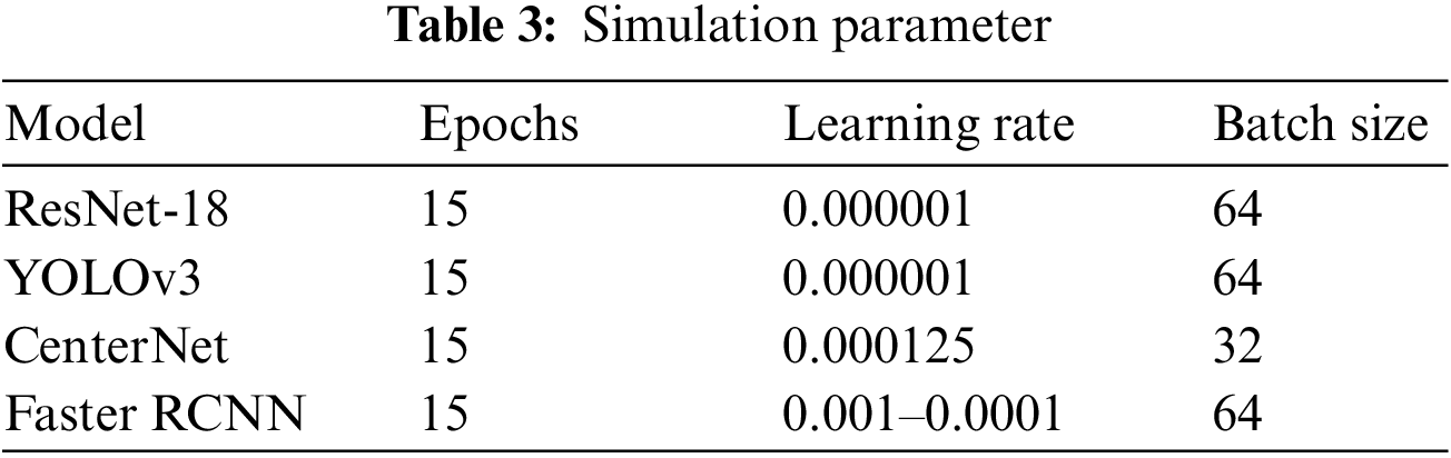
1. Due to the unfavorable effects of significant modifications to the deeper convolution filters, the low learning rate was chosen. Unfortunately, the learning process collapsed due to training with 0.000001 or 0.001 since the losses spiked to extremely high numbers and never returned.

2. As the largest value supported by an NVIDIA GPU, the batch size was chosen. This justification stems from the knowledge that bigger batch sizes offer a more precise gradient calculation for the weight update.

3. The number of training epochs for the custom models ranged from 10 to 25, and once overfitting was detected, the previous epoch was applied. Therefore, we have found that 15 epochs are the ideal number for this experiment for all the models.

4.2 Discussion

We evaluated the models on 1327 samples and got different IoU results for the four models we used. The test mean IoU score is shown in Table 4.

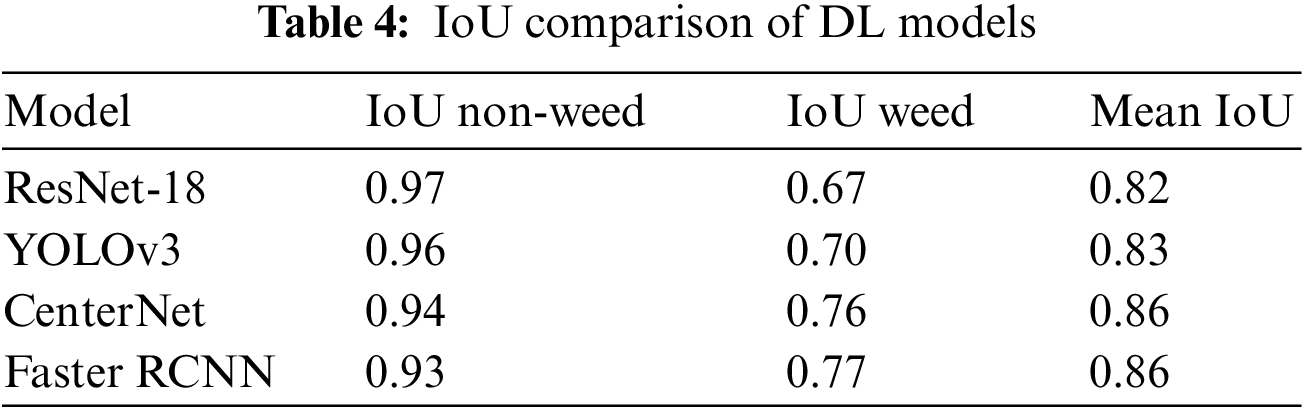
IoU compares the ground truth of the image we gave as an input and the model’s predicted mask generated from the input image. Hence, IoU gives the exact amount of overlap compared to the union. Fig. 9 summarizes models based on IoU non-weed, IoU weed, and MIoU measures for the test dataset. The IoU threshold is set to 0.70 for this experiment.

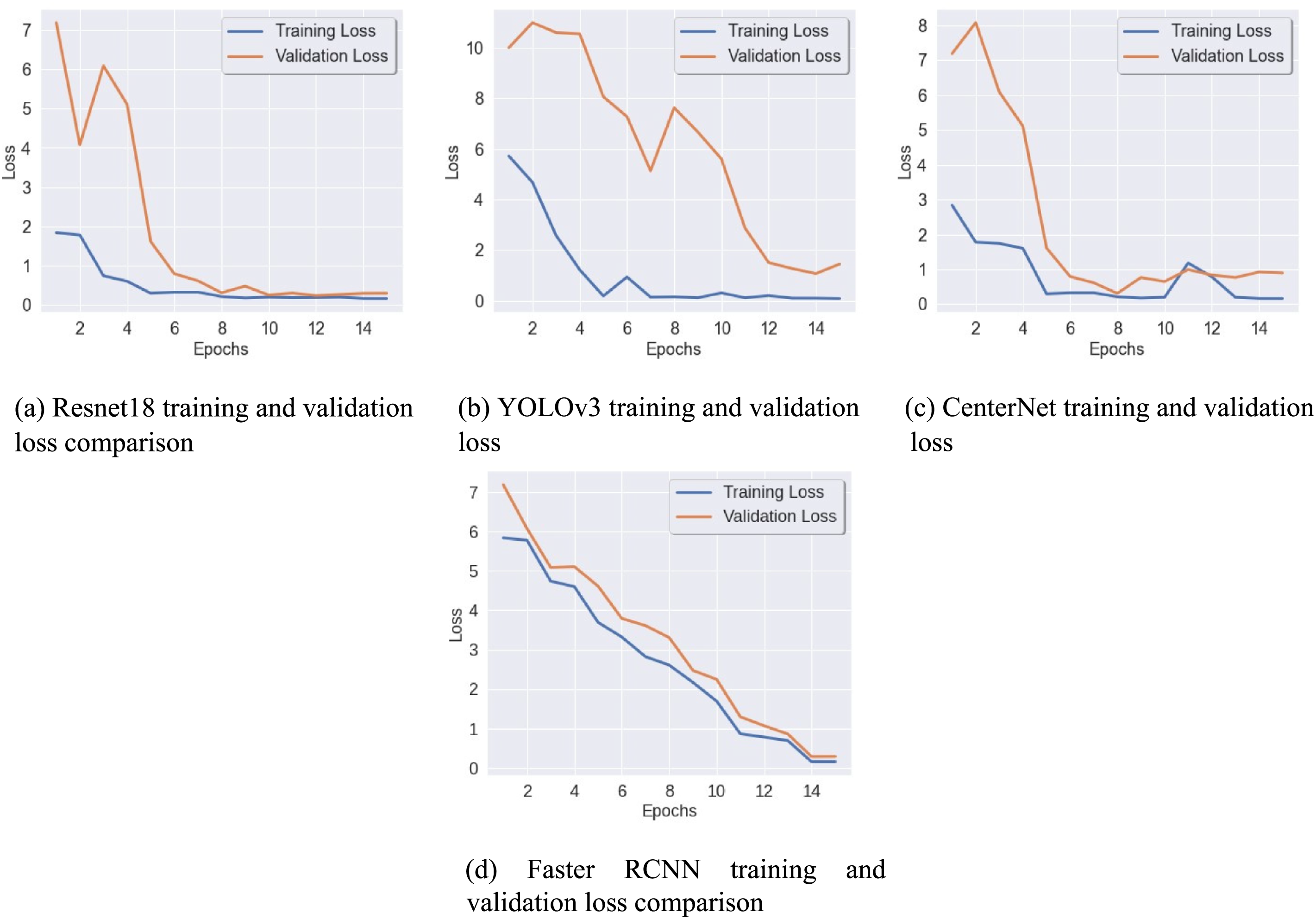
Figure 9: Training and validation loss analysis of the proposed AI models

Conditional Random Field (CRF) is implemented as a post-processing technique to improve the efficiency parameters by considering the neighboring predicted values. We have trained four different models with distinct backbone architectures. These segmentation models gave pretty good results when compared with each other. These models have simple architecture, faster training time, and simple implementation. The closure curves for all the models are shown in Fig. 9. We have trained all the models for 15 epochs based on the dataset size for training to avoid overfitting the model due to excessive training.

Epochs vs. Loss Graphs can be helpful in helping us to determine whether or not our model is overfitting or underfitting. For the YOLOv3 model, we might need to increase epochs because we can see that training and validation loss swings and that there is still some difference between training and validation even after 15 epochs. For ResNet18, we can observe that the graph appears inactive and that loss is also steadily dropping; after ten epochs, the difference between training and validation loss is nearly zero. We should apply this model to data that is differently distributed and make sure that it will not lead to any overfitting problems, according to the CenterNet graph, which shows that the starting training loss is quite low and has not decreased steadily. The model is learning gradually, but we can still run a few more epochs to ensure it doesn’t change much more and to check whether the difference between training loss and validation loss becomes null. We can observe in the Faster RCNN that the model begins training with a very high loss but that, over time, training and validation loss declines, resulting in an idle situation.

The authors have compared models based on three different parameters: first, the accuracy aspect, the memory usage aspect, and the IoU aspect. We conducted experiments using ResNet-18, YOLOv3, CenterNet, and Faster RCNN models. The performance of the model’s training is validated using a validation, where the ResNet18 model had the lowest accuracy of 81% and high training loss, as displayed in Table 5. During training, it appears to have detected the dataset’s imbalance, which is probably brought on by the lack of dropout regularisation. CenterNet outperformed all the models and achieved the highest accuracy at 88%. The reason behind good accuracy is to apply an effective scaling technique using compound coefficient and anchorless object detection. The idea behind the model is to focus on how much of the item it overlaps with; box predictions can be prioritized for significance based on their center only.

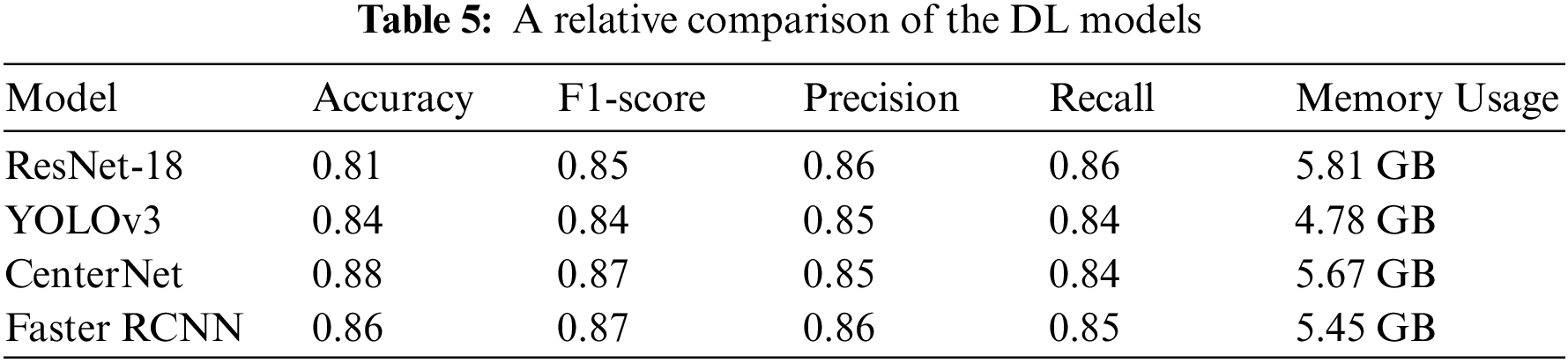
When compared to other models in the experiment, the ResNet-18 model requires somewhat more memory in terms of memory consumption. YOLOv3 is the lightest model as compared to all the models. It requires only 4.78 GB of memory to process the data. The main reason behind the vast difference is the depth and width of the network. YOLOv3 works with only 2M parameters, while ResNet-18 takes 11M. Regarding IoU non-weed, IoU weed, and mean IoU concerns, CenterNet and Faster RCNN achieve the same mean IoU of 0.86. As the predicted result shows, models are trained to capture the partition wall. These two architectures find the overlap between the weed-segmented area and the ground truth (manually generated).

5  Conclusion

Weed detection is an essential aspect of farming and, apart from other factors, affects crop yield and quality. This paper presents the comparative analytics of DL models to find weeds from the crop fields of the most popular vegetation crop, brinjal. Weed identification and detection require segregating soil, crop, and weed from an image. Data collection, preprocessing, data augmentation, classification, object detection, and postprocessing using CNN and DL models helped us achieve good results. The approach utilizes the pros of CNN in classification and DL in weed detection. With the help of the proposed model, we could classify the brinjal crop plant and detect weeds from the image given to the model with the best accuracy score of 88%. CenterNet is the most suitable architecture for brinjal weed detection among all the models, with a mean IoU of 86% and an accuracy of 88%. The memory requirement for ResNet-18 is quite higher than YOLOv3. The results are promising, and they provide a nod to achieving the objectives such as reducing herbicide usage and saving time from laborious hand weeding. These results also pave the way for the use of PA for site-specific weed management in vegetable crops. This work for weed detection in brinjal crops can be extended as a part of future work by developing an end-to-end pipeline. The pipeline would include a weed classification module that takes plant images as input. With the help of a classification module, it would classify the images into plant or non-plant (weed) types. It would then forward only the images of weed images to the object detection module to get the exact prediction mask, where the image is segmented into weed and plant. This would make a combination of classification and object detection, proving to be a perfect package for any application in real-time.

In the future, we will test the performance of the proposed model considering diversified parameters like latency and prediction time and integrate the new DL-based models, such as CoAtNet-7 and ModelSoups (Basic-L).

Acknowledgement: The authors would also like to acknowledge all members of Sudeep Tanwar’s Research Group (ST Lab) for their support in revising this manuscript. Further, the authors would like to acknowledge editorial board members of CMC and reviewers for providing technical comments to improve overall scientific depth of the manuscript.

Funding Statement: This work was funded by the Researchers Supporting Project Number (RSP2023R509), King Saud University, Riyadh, Saudi Arabia.

Author Contributions: The authors confirm contribution to the paper as follows: study conception and design: Jigna Patel, Anand Ruparelia, Sudeep Tanwar; data collection: Jigna Patel, Anand Ruparelia, Ravi Sharma; analysis and interpretation of results: Sudeep Tanwar, Maria Simona Raboaca, Bogdan Constantin Neagu, Fayez Alqahtani, Amr Tolba; draft manuscript preparation: Jigna Patel, Simona Raboaca, Bogdan Constantin Neagu. All authors reviewed the results and approved the final version of the manuscript.

Availability of Data and Materials: Not applicable.

Conflicts of Interest: The authors declare that they have no conflicts of interest to report regarding the present study.

References

1. Faostat, “Food and Agriculture Organization of the United Nations,” 2021. [Online]. Available: https://www.fao.org/faostat/en/?data. [Google Scholar]

2. Wikipedia, “List of countries and dependencies by population,” 2022. [Online]. Available: https://en.wikipedia.org/wiki/List_of_countries_and_dependencies_by_population. [Google Scholar]

3. Jagdish, “Growing eggplant from seeds-at home,” 2021. [Online]. Available: https://www.agrifarming.in/growing-eggplant-from-seeds-at-home. [Google Scholar]

4. A. Bakhshipour, A. Jafari, S. M. Nassiri and D. A. Zare, “Weed segmentation using texture features extracted from wavelet sub-images,” Biosystems Engineering, vol. 157, pp. 1–12, 2017. [Google Scholar]

5. E. AlJbawi, A. Mahmoud, F. Naom, A. G. Al-Khaldi and B. Al-Abdallah, “The response of morphological traits of sugar beet (beta vulgaris L) to different irrigation methods and nitrogen fertilization ratios,” Stem Cell Research International, vol. 4, no. 2, pp. 16–23, 2021. [Google Scholar]

6. E. C. Oerke, “Crop losses to pests,” The Journal of Agricultural Science, vol. 144, no. 1, pp. 31–43, 2006. [Google Scholar]

7. C. M. Benbrook, “Trends in glyphosate herbicide use in the United States and globally,” Environmental Science Europe, vol. 28, pp. 1–15, 2016. [Google Scholar]

8. M. H. Asad and A. Bais, “Weed detection in canola fields using maximum likelihood classification and deep convolutional neural network,” Information Processing in Agriculture, vol. 7, no. 4, pp. 535–545, 2020. [Google Scholar]

9. P. G. Kughur, “The effects of herbicides on crop production and environment in makurdi local government area of benue state, Nigeria,” Journal of Sustainable Development in Africa, vol. 14, no. 4, pp. 23–29, 2012. [Google Scholar]

10. J. P. Myers, M. N. Antoniou, B. Blumberg, L. Carroll, T. Everett et al., “Concerns over use of glyphosate-based herbicides and risks associated with exposures: A consensus statement,” Environmental Health, vol. 15, no. 1, pp. 1–13, 2016. [Google Scholar]

11. V. Kulkarni, “Government moves to restrict use of glyphosate,” The Hindu Business Line. 2020. [Online]. Available: https://www.thehindubusinessline.com/news/government-moves-to-restrict-use-ofglyphosate/article32029918.ece. [Google Scholar]

12. W. Kazmi, F. Garcia-Ruiz, J. Nielsen, J. Rasmussen and H. J. Andersen, “Exploiting affine invariant regions and leaf edge shapes for weed detection,” Computers and Electronics in Agriculture, vol. 118, pp. 290–299, 2015. [Google Scholar]

13. Ikisan, “Kisan,” 2022. [Online]. Available: https://www.ikisan.com/agri-informatics.html. [Google Scholar]

14. Y. K. Zhang, M. K. Wang, D. L. Zhao, C. Y. Liu and Z. G. Liu, “Early weed identification based on deep learning: A review, Smart Agricultural Technology,” vol. 3, pp. 100123, 2023. [Google Scholar]

15. P. Lottes, J. Behley, A. Milioto and C. Stachniss, “Fully convolutional networks with sequential information for robust crop and weed detection in precision farming,” IEEE Robotics and Automation Letters, vol. 3, no. 4, pp. 2870–2877, 2018. [Google Scholar]

16. J. Hemming and T. Rath, “PA—Precision agriculture,” Journal of Agricultural Engineering Research, vol. 78, no. 3, pp. 233–243, 2001. [Google Scholar]

17. A. Wang, Y. Xu, X. Wei and B. Cui, “Semantic segmentation of crop and weed using an encoder decoder network and image enhancement method under uncontrolled outdoor illumination,” IEEE Access, vol. 8, pp. 81724–81734, 2020. [Google Scholar]

18. S. Taghadomi-Saberi and A. Hemmat, “Improving field management by machine vision–A review,” Agricultural Engineering International: CIGR Journal, vol. 17, no. 3, pp. 92–111, 2015. [Google Scholar]

19. E. C. Oerke, R. Gerhards, G. Menz and R. A. Sikora, Precision Crop Protection-The Challenge and Use of Heterogeneity, vol. 5. Dordrecht: Springer, pp. 1–24, 2010. [Google Scholar]

20. K. Sheth, K. Patel, H. Shah, S. Tanwar, R. Gupta et al., “A taxonomy of AI techniques for 6G communication networks,” Computer Communications, vol. 161, pp. 279–303, 2020. [Google Scholar]

21. F. Lopez-Granados, “Weed detection for site-specific weed management: Mapping and real-time approaches,” Weed Research, vol. 51, no. 1, pp. 1–11, 2011. [Google Scholar]

22. J. Tang, D. Wang, Z. Zhang, L. He, J. Xin et al., “Weed identification based on K-means feature learning combined with convolutional neural network,” Computers and Electronics in Agriculture, vol. 135, pp. 63–70, 2017. [Google Scholar]

23. R. Gerhards, D. Andújar Sanchez, P. Hamouz, G. G. Peteinatos, S. Christensen et al., “Advances in site-specific weed management in agriculture—A review,” Weed Research, vol. 62, pp. 123–133, 2022. [Google Scholar]

24. A. Rahman, Y. Lu and H. Wang, “Performance evaluation of deep learning object detectors for weed detection for cotton,” Smart Agricultural Technology, vol. 3, pp. 1–11, 2023. [Google Scholar]

25. A. Minhas, “Gross value added from agriculture, forestry and fishing in India from financial year 2012 to 2020,” Statista Research Department. 2022. [Online]. Available: https://www.statista.com/statistics/805180/india-real-gva-in-agriculture-forestry-and-fishing-sector/. [Google Scholar]

26. The World Bank, “India: Issues and priorities for agriculture,” 2012. [Online]. Available: https://www.worldbank.org/en/news/feature/2012/05/17/india-agriculture-issues-priorities. [Google Scholar]

27. J. M. Alston and P. G. Pardey, “Agriculture in the global economy,” The Journal of Economic Perspectives, vol. 28, no. 1, pp. 121–146, 2014. [Google Scholar]

28. X. Jin, J. Che and Y. Chen, “Weed identification using deep learning and image processing in vegetable plantation,” IEEE Access, vol. 9, pp. 10940–10950, 2021. [Google Scholar]

29. J. Patel, R. Patel, S. Shah and J. Patel, “Big data analytics for advanced viticulture,” Scalable Computing: Practice and Experience, vol. 22, pp. 303–312, 2021. [Google Scholar]

30. Markets and Markets, “Artificial intelligence in agriculture market,” 2022. [Online]. Available: https://www.marketsandmarkets.com/Market-Reports/ai-in-agriculture-market-159957009.html. [Google Scholar]

31. E-Lab, “E-lab/pytorch-linknet,” 2018. GitHub. [Online]. Available: https://github.com/e-lab/pytorch-linknet. [Google Scholar]

32. Wikipedia, “Weed control,” 2022. [Online]. Available: https://en.wikipedia.org/wiki/Weed_control. [Google Scholar]

33. R. Raja, T. T. Nguyen, V. L. Vuong, D. C. Slaughter and S. A. Fennimore, “RTD-SEPs: Real-time detection of stem emerging points and classification of crop-weed for robotic weed control in producing tomato,” Biosystems Engineering, vol. 195, pp. 152–171, 2020. [Google Scholar]

34. N. Wang, N. Zhang, J. Wei, Q. Stoll and D. Peterson, “A real-time, embedded, weed detection system for use in wheat fields,” Biosystems Engineering, vol. 98, no. 3, pp. 276–285, 2007. [Google Scholar]

35. S. Tanwar, T. Ramani and S. Tyagi, “Dimensionality reduction using PCA and SVD in big data: A comparative case study,” in Int. Conf. on Future Internet Technologies and Trends, pp. 116–125, 2018. [Google Scholar]

36. J. Torres-Sospedra and P. Nebot, “Two-stage procedure based on smoothed ensembles of neural networks applied to weed detection in orange groves,” Biosystems Engineering, vol. 123, pp. 40–55, 2014. [Google Scholar]

37. S. Hameed and I. Amin, “Detection of weed and wheat using image processing,” in IEEE 5th Int. Conf. on Engineering Technologies and Applied Sciences (ICETAS), Bangkok, Thailand, pp. 1–5, 2018. [Google Scholar]

38. A. Dos Santos Ferreira, D. M. Freitas, G. G. da Silva, H. Pistori and M. T. Folhes, “Weed detection in soybean crops using convnets,” Computers and Electronics in Agriculture, vol. 143, pp. 314–324, 2017. [Google Scholar]

39. A. Bakhshipour and A. Jafari, “Evaluation of support vector machine and artificial neural networks in weed detection using shape features,” Computers and Electronics in Agriculture, vol. 145, pp. 153–160, 2018. [Google Scholar]

40. T. Ashraf and Y. N. Khan, “Weed density classification in rice crop using computer vision,” Computers and Electronics in Agriculture, vol. 175, pp. 1–7, 2020. [Google Scholar]

41. L. Duncan, B. Miller, C. Shaw, R. Graebner, M. L. Moretti et al., “Weed warden: A low-cost weed detection device implemented with spectral triad sensor for agricultural applications,” HardwareX, vol. 11, pp. 1–19, 2022. [Google Scholar]

42. A. Subeesh, S. Bhole, K. Singh, N. S. Chandel, Y. A. Rajwade et al., “Deep convolutional neural network models for weed detection in polyhouse grown bell peppers,” Artificial Intelligence in Agriculture, vol. 6, pp. 47–54, 2022. [Google Scholar]

43. M. Perez-Ortiz, J. Pena, P. Gutierrez, J. Torres-Sanchez and C. Hervas-Martinez, “A semi-supervised system for weed mapping in sunflower crops using unmanned aerial vehicles and a crop row detection method,” Applied Soft Computing, vol. 37, pp. 533–544, 2015. [Google Scholar]

44. V. Partel, S. Charan Kakarla and Y. Ampatzidis, “Development and evaluation of a low-cost and smart technology for precision weed management utilizing artificial intelligence,” Computers and Electronics in Agriculture, vol. 157, pp. 339–350, 2019. [Google Scholar]

45. K. Hu, G. Coleman, S. Zeng, Z. Wang and M. Walsh, “Graph weeds net: A graph-based deep learning method for weed recognition,” Computers and Electronics in Agriculture, vol. 174, pp. 1–9, 2020. [Google Scholar]

46. P. Bosilj, T. Duckett and G. Cielniak, “Analysis of morphology-based features for classification of crop and weeds in precision agriculture,” IEEE Robotics and Automation Letters, vol. 3, no. 4, pp. 2950–2956, 2018. [Google Scholar]

47. C. Shorten and T. Khoshgoftaar, “A survey on image data augmentation for deep learning,” Journal of Big Data, vol. 6, no. 1, pp. 1–48, 2019. [Google Scholar]

48. A. Rosebrock, “Intersection over Union (IOU) for object detection,” pyimagesearch. 2016. [Online]. Available: https://pyimagesearch.com/2016/11/07/intersection-over-union-iou-for-object-detection/. [Google Scholar]

49. Phacelia, “Eggplant-brinjal-World Crops Database,,” 2021. [Online]. Available: https://world-crops.com/eggplant/. [Google Scholar]

50. Native Plant Trust: Go Botany, “Solanum melongena-eggplant,” 2022. [Online]. Available: https://gobotany.nativeplanttrust.org/species/solanum/melongena/. [Google Scholar]

51. “485 brinjal tree stock photos, images & pictures,” 2022. [Online]. Available: https://www.dreamstime.com/photos-images/brinjal-tree.html. [Google Scholar]

52. Kaggle, “Find Open Datasets and Machine Learning Projects,” 2022. [Online]. Available: https://www.kaggle.com/datasets. [Google Scholar]

53. H. Jeon, L. Tian and H. Zhu, “Robust crop and weed segmentation under uncontrolled outdoor illumination,” Sensors, vol. 11, no. 6, pp. 6270–6283, 2011. [Google Scholar] [PubMed]

54. “Unet for image segmentation,” GitHub. 2019. [Online]. Available: https://github.com/zhixuhao/unet. [Google Scholar]

55. A. Wang, W. Zhang and X. Wei, “A review on weed detection using ground-based machine vision and image processing techniques,” Computers and Electronics in Agriculture, vol. 158, pp. 226–240, 2019. [Google Scholar]

56. J. Chen, H. Wang, H. Zhang, T. Luo and D. Wei, “Weed detection in sesame fields using a yolo model with an enhanced attention mechanism and feature fusion,” Computers and Electronics in Agriculture, vol. 202, no. 4, 12, pp. 1–12, 2022. [Google Scholar]

57. X. Jin, Y. Sun, J. Che, M. Bagavathiannan and J. Yu, “A novel deep learning-based method for detection of weeds in vegetables,” Pest Management Science, vol. 78, no. 5, pp. 1861–1869, 2022. [Google Scholar] [PubMed]

58. A. Krizhevsky, I. Sutskever and G. E. Hinton, “ImageNet classification with deep convolutional neural networks,” Communications of the ACM, vol. 60, no. 6, pp. 84–90, 2017. [Google Scholar]

59. L. Q. Zhong, L. R. Li and G. Yang, “Characterizing robustness of deep neural networks in semantic segmentation of fluorescence microscopy images,” TechRxiv, 2022. [Google Scholar]

60. X. Ma, X. Deng, L. Qi, Y. Jiang, H. Li et al., “Fully convolutional network for rice seedling and weed image segmentation at the seedling stage in Paddy Fields,” PLoS One, vol. 14, no. 4, pp. 1–13, 2019. [Google Scholar]

61. S. Khan, M. Tufail, M. Khan, Z. Ahmad and S. Anwar, “Deep learning-based identification system of weeds and crops in strawberry and pea fields for a precision agriculture sprayer,” Precision Agriculture, vol. 22, pp. 1–17, 2021. [Google Scholar]

62. J. Redmon, “YOLO: Real-time object detection,”. 2022. [Online]. Available: https://pjreddie.com/darknet/yolo/. [Google Scholar]

63. Ultralytics, “Ultralytics/yolov3: YOLOv3 in PyTorch,” GitHub. 2022. [Online]. Available: https://github.com/ultralytics/yolov3. [Google Scholar]

64. X. Deng, “Object detection of alternanthera philoxeroides at seedling stage in paddy field based on Faster R-CNN,” in IEEE 5th Advanced Information Technology, Electronic and Automation Control Conf. (IAEAC), Chongqing, China, pp. 1125–1129, 2021. [Google Scholar]

65. F. Cao and Q. Bao, “A survey on image semantic segmentation methods with convolutional neural network,” in Int. Conf. on Communications, Information System and Computer Engineering (CISCE), Kuala Lumpur, Malaysia, pp. 458–462, 2020. [Google Scholar]