Rail Surface Defect Detection Based on Improved UPerNet and Connected Component Analysis

1  Introduction

In the intricate wheel-rail system, the rail serves dual pivotal roles: it bears the vehicular vertical load and facilitates guidance. The rail head, consequent to this, encounters longitudinal and transverse forces, engendering vibrations throughout the rail system. Such perturbations can lead to detrimental surface defects on the rail. Notably, these imperfections intensify the rail’s vertical vibrations, transmitting these oscillations to the locomotive. This amplification can heighten the potential for resonance between the vehicle and its assorted elastic components. Concurrently, an increase in the rail’s torque can be observed, undermining the wheel’s directional function and jeopardizing the vehicle’s lateral stability. Hence, prompt detection of these rail surface defects becomes imperative [1].

The vast expanse of the railway network, coupled with a multifarious natural environment and dense departures, renders manual inspection an inefficacious solution. However, the advancement in machine vision coupled with the burgeoning field of deep learning has catapulted non-contact, image-based defect detection methods into a focal research area. Traditional visual techniques predominantly utilize texture and rudimentary grayscale attributes to discern and pinpoint target zones in unlabeled rail samples. Classic methodologies employ a gradient histogram in tandem with support vector machines, realizing rail surface defect detection. This can be further amalgamated with multiple detectors within a multi-task learning paradigm to enhance detection prowess [2]. A notable study by Li et al. [3] has accentuated defect contrasts via local normalization and defect proportion limitation filtering. Their approach employed a grayscale projection contour algorithm, displaying robustness to noise, with the added advantage of swift detection rates. Techniques encompassing the internal point hollowing algorithm, coupled with the chain code tracking algorithm, have demonstrated potential in capturing defect contour data, thereby enabling automated detection of rail surface defect regions [4]. In another significant research [5], differentiation of the rail image post-inverse Perona-Malik (P-M) diffusion from the prototypical image was undertaken to minimize environmental interferences. Following this, the defect region was segmented through an edge feature-based filtering algorithm. To further refine the segmentation threshold of rail defects, a novel Otsu method integrating target variance weighting was introduced in [6]. Some researchers have applied Laplace low-pass filtering to rail imagery, subsequently differentiating it from the original image. This was followed by morphological feature extraction for defect detection. On average, the accuracy of this methodology was found to be 85.3% [7]. Yaman et al. [8] adopted a distinctive approach by extracting feature types from the variance signal of rail imagery, subsequently ascertaining the fault type via fuzzy logic. In light of the insensitivity of defect detection to the rail’s transverse luminosity alterations, a defect detection framework was formulated. This system, underpinned by morphological operators, employed elongated, slender structural elements aligned parallel to the rail’s longitudinal axis for image processing, effectively curtailing false positives [9]. Confronting the challenges inherent in rail detection, such as intricate conditions and unequal rail luminescence, a region extraction algorithm hinged on vertical projection and grayscale differentiation was conceptualized. Furthermore, an enhanced rapid robust Gaussian mixture model anchored on the Markov random field was designed, aiming for swift and precise surface defect segmentation [10]. Academic discourse has also illuminated a maximum entropy threshold segmentation technique. This method, rooted in the principle where the background entropy remains invariant in low gray domains, while the target entropy fluctuates in accordance with the gray scale, has shown promise in attaining optimal thresholds for demarcating rail surface defects [11]. It is crucial to note, however, that while these methods have advanced defect object detection considerably, they demand scene-specific modifications. Thus, their adaptability and real-time performance warrant further enhancement.

Deep learning methodologies employ convolutional neural networks (CNNs) to represent defects in rail images as abstract digital features for enhanced detection. The prevailing research predominantly capitalizes on object detection and semantic segmentation networks, epitomized by their rapid processing capabilities and obviation of manual feature setting. Certain approaches harness CNNs directly to categorize rail surface defects for detection intentions. For instance, a study delineated in [12] contrived a CNN comprised of 2 convolution layers, 2 pooling layers, and a fully connected layer, expressly for rail surface defect detection; a regularization technique was incorporated during the training phase to augment the recognition rate. Faghih-Roohi et al. [13], in their exploration, classified rail defect images into six distinct categories and embarked on training three disparate structures of deep CNNs via the small batch gradient descent approach. Their findings underscored the superior classification performance of more profound network structures, with heightened accuracy when the rectified linear unit (ReLU) was integrated into training.Turning to detection methodologies based on semantic segmentation networks, a study referenced in [14] conceived a 59-layer semantic segmentation network rooted in the SegNet architecture to pinpoint rail surface anomalies. When juxtaposed against the Otsu segmentation and manual threshold segmentation techniques, this semantic segmentation network triumphed with the preeminent detection rate. Further, a study in [15] introduced a lightweight rail surface defect detection network that synergized MobileNetV2 with the You Only Look Once version3 (YOLOv3) mechanism. By supplanting Darknet53 with MobileNetV2 for backbone extraction, and concurrently designing a multi-scale predictor inspired by target regression, an inference speed culminating at 87.40% mean average precision (mAP) and 60 frames per second (FPS) was realized. Jin et al. [16] amalgamated semantic segmentation with object detection techniques within their detection framework, integrating Dropout with Xception—a backbone network of DeepLabV3+. To counteract the pixel imbalance between the foreground and background, YOLO was employed to pinpoint defects and deduce foreground and background weighting coefficients, thereby furnishing attention loss for the segmentation model. Dilated convolution emerges as a prevalent strategy to amplify the receptive field. A paper cited in [17] devised a lightweight semantic segmentation model rooted in a cascading self-encoding network for defect detection in rails and crafted a compact CNN specifically for defect classification. This methodology flourished both in detection precision and temporal efficiency. Luo et al.’s works [18,19] incorporated dilated convolution into the Faster Regions with CNN Features (Faster R-CNN) and established parallel convolution channels, each with unique expansion coefficients catering to distinct defect types. This innovation bolstered the detection precision of nuanced defects. Subsequent investigations leveraged the Cascade Regions with CNN Features (Cascade R-CNN) for rail surface defect detection. Addressing challenges like the skewed distribution of sample IoU and misalignment between regions of interest and feature maps engendered by rounding quantization, and the inaccurate prognostication of regression boundaries, various tools such as IoU balanced sampling, region of interest aligns (RoIAlign), and complete intersection over union (CIoU) loss were assimilated to hone the average precision (AP) to a staggering 98.75%. While unsupervised methodologies have also been ventured into for rail surface defect detection, their prevalence remains limited. A study in [20], for example, employed scale normalized cross fast flow for probability distribution estimation, which facilitated the derivation of an image’s standard Gaussian distribution. Anomaly scores were subsequently discerned based on the proximity to the distribution’s epicenter, serving the dual purpose of detection and defect localization.

Currently, the rail surface defect detection employing image methodologies confronts several challenges: (a) The discernible information present within rail images is somewhat circumscribed, leading to diminished efficiency of methods grounded on texture and grayscale features. (b) The proactive maintenance interventions by the concerned departments hinder the effective accumulation of a voluminous dataset of rail defect images, thereby compromising the efficacy of supervised deep learning. (c) Although a plethora of rail inspection vehicles are competent in detecting fastener defects, the image data they procure for rail damage differs significantly from conventional images, making them unsuitable for direct utilization. (d) Rail surface anomalies predominantly manifest in two distinct forms: ripple and discrete defects. The emergence of discrete defects is characterized by their unpredictability, arbitrariness, and multi-scale dimensions, devoid of any recurring patterns, which intensifies the challenges associated with defect detection [21]. (e) The intricate edge configurations of rail surface defects pose considerable challenges to semantic segmentation algorithms. (f) The detection outcomes yielded by deep learning approaches are arduous to correlate directly with the specific parameters delineating the defects.

In light of these challenges, an enhanced UPerNet semantic segmentation network was introduced specifically for rail defect detection. Concurrently, a Swin-T network integrating the Transformer architecture was deployed for the extraction of defect features, which capitalized on the holistic information embedded within the images while circumventing the issue of inductive bias. The rule window self-attention inherent in Swin-T mitigates the model’s parameter load. Additionally, the cross-GPU synchronized batch normalization technique was harnessed for gradient refinement, with Lovász-hinge being employed as the loss function, facilitating the leveraging of inter-pixel dependency relationships. Conclusively, grounded on the semantic segmentation imagery of rail surface anomalies, the distinct defect regions were identified via connected component analysis, enabling the computation of the genuine length and area of the defects.

The contributions of this research can be dichotomized as:

(a) The proposition of a rail surface defect detection algorithm founded on semantic segmentation. Within this framework, the Swin-T, encompassing the Transformer architecture, is incorporated, amplifying the capability of the segmentation network in the extraction of rail surface defect features, and bolstering the defect segmentation quality. Notwithstanding the pervasive application of Transformers across a myriad of visual tasks—attributed to their prowess in assimilating global context information—their deployment for this specific endeavor remains an exception.

(b) Pivoting from the semantic segmentation representations of rail surface anomalies, connected component analysis is integrated, which adeptly bridges the detection outcomes of the deep learning modus operandi with the intricate parameters defining the defects. Such an approach aids railway maintenance personnel in intuitively grasping the defect metrics, enabling them to orchestrate targeted remediation measures.

2  Related Work

2.1 Transformer

The Transformer architecture, a manifestation of the encoder-decoder network paradigm, is predominantly anchored on the attention mechanism [22]. Dispensing with recursion and convolution, it rectifies the inherent sluggishness that plagues the training of Recurrent Neural Networks (RNN) and has demonstrated its proficiency in machine translation endeavors. Models grounded in the Transformer architecture, such as Bidirectional Encoder Representation from Transformers (BERT) [23] and Generative Pre-train Transformer (GPT) [24], have been recognized for their stellar performance in the realm of natural language processing. For myriad computer vision tasks, the prototypical Transformer encoder model is employed, serving as a novel feature extraction apparatus. The Vision Transformer (ViT) [25], designed for image classification, segments images into standardized image blocks. These embedded blocks are subsequently input into the Transformer encoder, and post Multilayer Perceptron (MLP) classification processing, it garners commendable results, rivaling top-tier convolutional networks. The DEtection TRansformer (DETR) [26] amalgamates both CNN and Transformer architectures to present an end-to-end object detection framework, reframing object detection as a images-to-sets prediction conundrum. By leveraging the self-attention mechanism of the Transformer, it simulates all pairwise interactions amidst elements in a sequence, rendering it more conducive for the intricate constraints intrinsic to set prediction. Chen et al. [27] devised the Image Processing Transformer (IPT), a model sculpted on the Transformer architecture, adept at addressing image processing challenges, excelling in tasks like image super-resolution, restoration, and denoising across a plethora of marred images from ImageNet. As per Reference [28], a semi-supervised video segmentation blueprint was proffered, which incorporated the Transformer at its bottleneck layer to further distill contextual data, thereby enhancing the precision of endoscopic video segmentation in scenarios characterized by scarce annotated data. Despite the widespread adoption and commendation of the Transformer structure across a variety of visual tasks, attributed to its prowess in gleaning global contextual features, its deployment in the domain of rail surface defect detection remains limited.

2.2 Attention Mechanism

The genesis of the attention mechanism can be traced back to studies delving into human visual cognition. Given the constraints imposed by information processing bottlenecks, humans innately zero in on certain segments of the information spectrum, while disregarding the remainder. Emulating this intrinsic human trait, the attention mechanism in deep learning serves as an intuitive resource distribution conduit, reallocating weights contingent on the perceived significance of entities.

The Transformer intricately weaves multiple self-attention layers, culminating in multi-head self-attention (MSA), with an aim to enhance network efficiency, as depicted in Fig. 1. The self-attention layer transmutes the input vector into three distinct entities: the query vector (q), the key vector (k), and the value vector (v), subsequently coalescing them into three matrices: Q, K, and V. Attention weights are ascertained through a liaison between Q and K, and subsequently, the comprehensive weight and output are procured via their interaction with V. Vectors deemed of higher significance are accorded heightened attention in subsequent layers. The self-attention dynamic across disparate input vectors is delineated in formula (1), where dk represents the dimension pertinent to K.

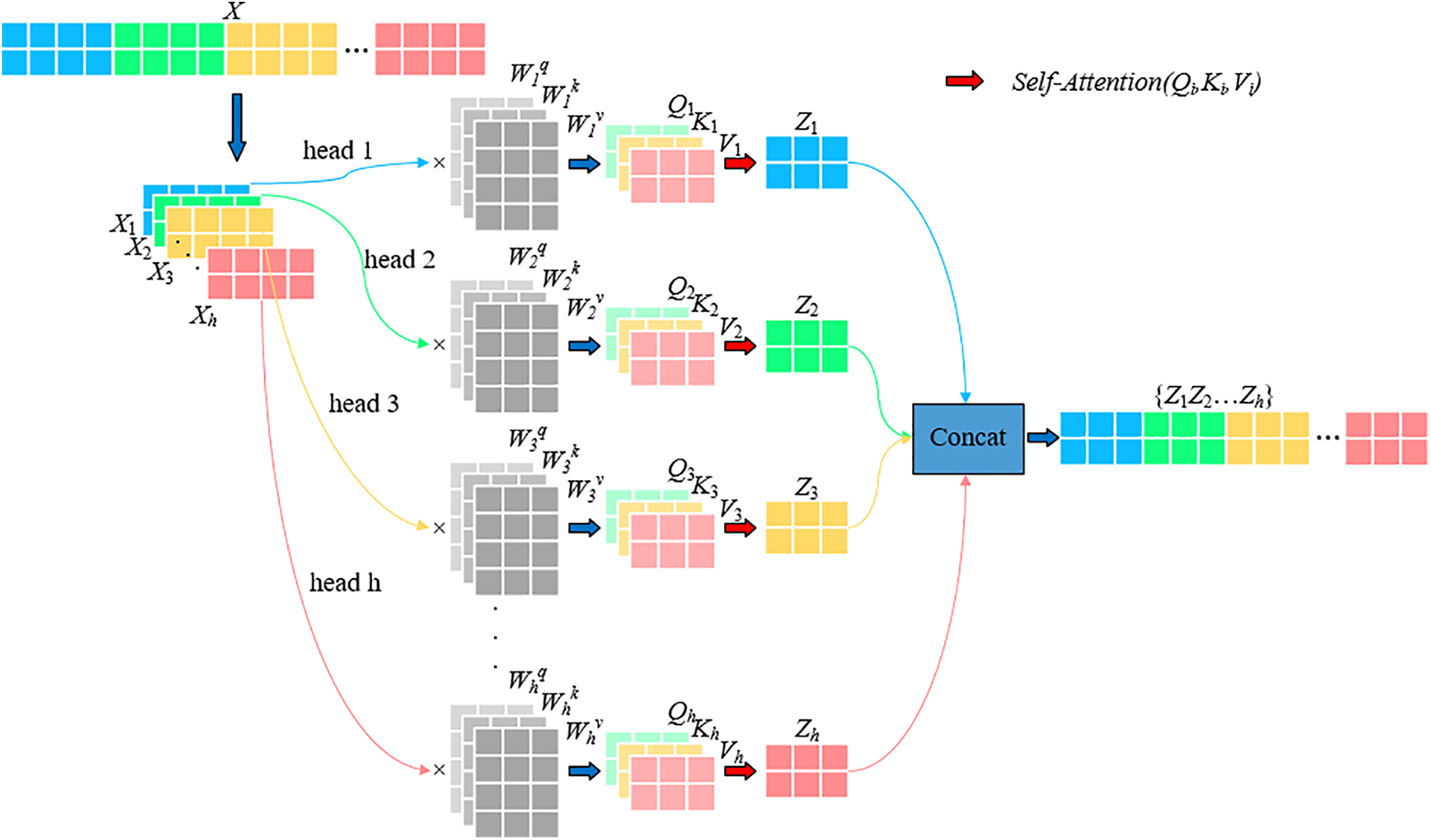
Figure 1: The principle of multi-head self-attention mechanism

Attention(Q,K,V)=softmax(Q⋅KTdk)⋅V(1)

The concept of multi-head self-attention gives rise to the simultaneous execution of multiple self-attention operations on features within the network. These individual operations are subsequently amalgamated to produce the final output, enabling the network to encapsulate a richer spectrum of feature information. This process is mathematically articulated in formula (2).

MultiHead(Q,K,V)=Concat(head1,…headh)WO(2)

where, headi is the result of each self-attention action, as shown in formula (3), WiQ, WiK and WiV are all projection weight matrices.

headi=Attention(QWiQ,KWiK,VWiV)(3)

3  Proposed Methodology

The UPerNet [29], a semantic segmentation network, is predicated upon both the Pyramid Pooling Module (PPM) and the Feature Pyramid Networks (FPN). Drawing upon four distinct feature layers as elucidated by ResNet, it meticulously weaves together multi-scale information derived from various stages, ensuring a minimized loss of boundary information. This is a marked improvement over the Pyramid Scene Parsing Network (PSPNet) [30], another network subscribing to the FPN framework. Yet, the UPerNet’s reliance on CNN for feature extraction manifested an inherent inductive bias, hindering the holistic utilization of global information. Moreover, when training is undertaken on a solitary GPU with a comparably smaller batch, the application of BN (Batch Normalization) tends to compromise the model’s convergence efficacy. Further, the employment of the cross-entropy loss function overlooks the intricate dependencies present amongst adjacent pixels. In light of these challenges, enhancements were made to the UPerNet, with its overarching structure delineated in Fig. 2. The encoder network, seeking refuge in Swin-T [31] for feature extraction, collaborates with the decoder network, which harnesses both PPM and FPN. This ensures a seamless projection of discernible features into the pixel space, post-upsampling. The final ensemble of feature maps, stemming from each stage of the feature extraction network, is encapsulated as {S2, S3, S4, S5}. Concurrently, the feature mapping borne out of the FPN output is represented as {P2, P3, P4, P5}, with P5 also succeeding PPM directly.

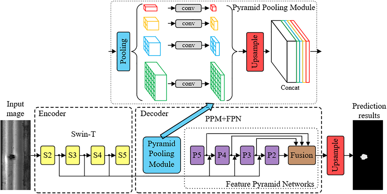
Figure 2: The overall structure of the method in this paper

3.1 Backbone Network

While CNNs have demonstrated proficiency across various image processing tasks, the inherent locality of convolutional operations and the inductive bias stemming from weight sharing impose constraints on long-distance dependencies. Such limitations curtail the ability of CNNs to glean comprehensive insights from an entire image and to facilitate information exchange beyond the confines of the convolutional kernel. In stark contrast, the self-attention mechanism inherent in the Transformer can adaptively modify its receptive domain, thereby furnishing long-range dependencies and circumventing the inductive bias endemic to CNNs. In this study, the Swin-T architecture is employed as the backbone network, facilitating the extraction of expansive global information and more nuanced features. The strategic confinement of attention computation to non-overlapping local windows ensures the computational complexity remains linear in relation to image size, thereby optimizing computational efficiency. A schematic representation of this network structure can be perused in Fig. 3.

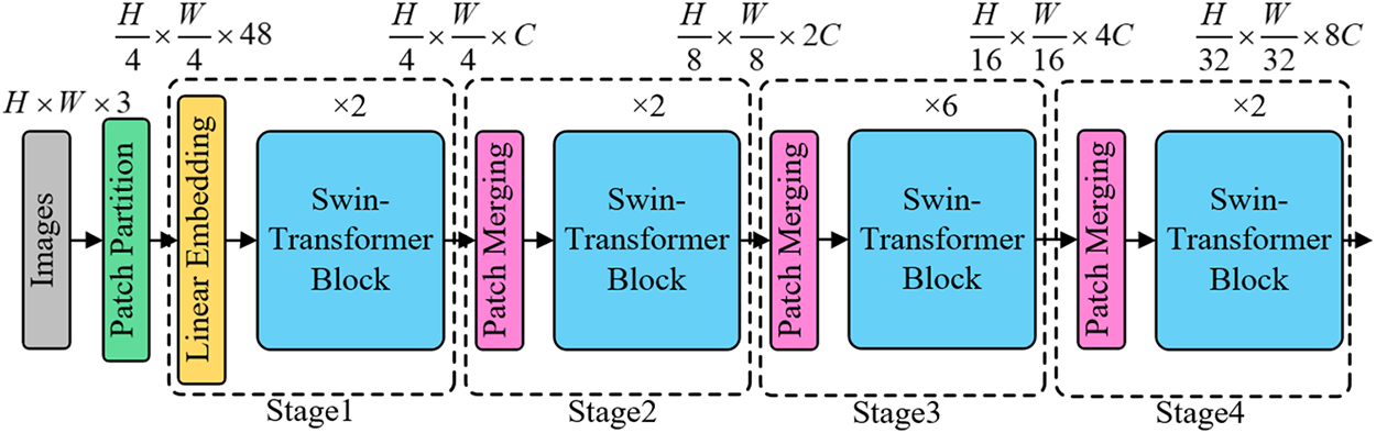
Figure 3: Network structure of Swin-T

The entire network adopts a stratified approach. Initially, an input image of dimensions H × W × 3 is partitioned into (H/4) × (W/4) non-overlapping patches via the patch-splitting module, subsequently flattening each patch into a 48-dimensional token vector. This is followed by the linear embedding layer projecting the tensor of dimensions (H/4) × (W/4) × 48 to an arbitrary dimension C, culminating in a linear mapping of dimension (H/4) × (W/4) × C. These mapped tokens are then channelled into the dual Swin Transformer module, which ensures the token count remains consistent at (H/4) × (W/4) both at the input and output. The inaugural Swin Transformer module, in conjunction with the linear embedding layer, is designated as the primary layer. Thereafter, the patch merging layer collaborates with the Swin Transformer module across subsequent layers to elucidate feature descriptors across varied scales.Swin Transformer diverges from traditional architectures like ResNet, opting to segregate the input image via diminutive windows, consequently parsing it into equitably sized blocks termed local windows. Within each of these local windows, feature extraction ensues, thereby permitting both self-attention and localized convolutional operations to ascertain feature information across diverse scales and positions. numerous Swin Transformer Blocks (analogous to the basic blocks in ResNet) are harnessed for feature extraction across Stages 2–4. Eschewing the simplistic stacking of convolutional layers as observed in ResNet, Swin Transformer adopts a hierarchical group convolution to optimize feature amalgamation. Furthermore, Swin Transformer facilitates inter-window information exchange, enhancing the context-dependence of features. As the network becomes progressively intricate, every layer metamorphoses the tensor’s dimension, culminating in a stratified representation. Pertinently, each patch boasts a size of 4, each self-attention window spans 7, and the network depth across the four blocks is catalogued as [2,2,6,2]. In summation, the multifaceted stages of Swin Transformer utilize local windows, hierarchical group convolution, and inter-window connections to glean feature insights across an array of positions and scales. This epitomizes Swin Transformer’s adeptness in tailoring its feature extraction capabilities to cater to diverse tasks and datasets.

The Swin Transformer Block is composed of Layer Normalization (LN), a multi-head self-attention module, a shortcut connection, and an MLP featuring a Gaussian Error Linear Unit (GELU) activation function. A representation of two consecutively arranged Swin Transformer Blocks is depicted in Fig. 4. Within the design of the multi-head self-attention module, the self-attention mechanism is intricately integrated into the window, encompassing two distinct types: the window-based self-attention (W-MSA) and the shifted window-based self-attention (SW-MSA). The W-MSA mode partitions the image into multiple windows and executes self-attention computations individually for each window. Given an image fragmented into h × w patches, where each window comprises M × M patches, the computational complexities of MSA and W-MSA are elucidated in formulas (4) and (5), respectively. A noteworthy reduction in computational complexity is achieved through W-MSA. Owing to the fact that the patch count within each window is significantly inferior to the total patch count of the image, the computational complexity associated with W-MSA exhibits linearity with respect to the image’s dimensions.

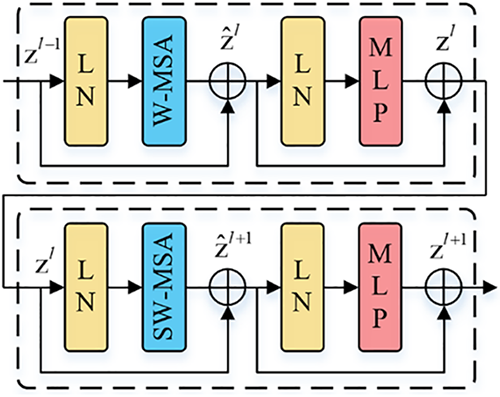
Figure 4: Two swin Transformer blocks in series

Ω(MSA)=4hwC2+2(hw)2C(4)

Ω(W−MSA)=4hwC2+2M2hwC(5)

SW-MSA, on the other hand, incorporates a shifted window approach, facilitating inter-window connections. This not only augments information transfer across different windows but also amplifies the receptive field, thereby bolstering the model’s representational prowess. The interrelationships embedded within the two serially arranged Swin Transformer Blocks are expounded in formula (6), where z^l and zl represent the features output by the two types of window self-attention and the features output by the MLP, respectively.

{z^l=W−MSA(LN(zl−1))+zl−1zl=MLP(LN(z^l))+z^lz^l+1=SW−MSA(LN(zl))+zlzl+1=MLP(LN(z^l+1))+z^l+1(6)

3.2 Synchronized Batch Normalization

In traditional applications, when batch normalization (BN) serves as the chosen normalization technique, the input x = {x1,x2,x3,x4} is segmented into multiple portions during each iteration of network training. These portions undergo forward and backward propagation processes, with the gradients being computed on disparate GPUs. Subsequently, a succeeding iteration is commenced post the amalgamation of gradients and parameters. This fundamental operation is visualized in Fig. 5.

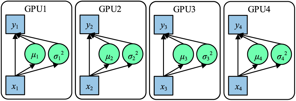
Figure 5: Working principle of BN

Due to each GPU processing data individually during both forward and backward propagations, the BN operation is independently executed on every GPU. Intrinsically, the samples normalized via BN are confined to their respective GPU, mirroring a reduction in the batch_size. A diminished batch_size can lead to the calculated mean and variance failing to capture the holistic data distribution, as a smaller batch_size introduces heightened variability. Notably, in the realm of deep learning, an expansive batch_size typically stabilizes the training trajectory. Cross-GPU synchronized batch normalization (SyncBN) retrieves the universal mean μ and variance σ2 during the forward propagation phase, and computes the overarching gradient throughout the backward propagation. When deducing the global gradient in the backward propagation, the global BN statistics can be employed for input normalization, which invariably refines the accuracy of these statistics, as depicted in Fig. 6.

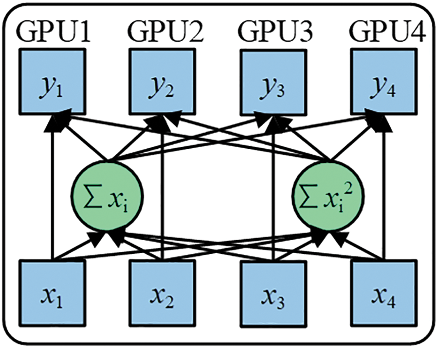
Figure 6: Working principle of SyncBN

SyncBN ensures that the input data distribution across every network layer remains comparably consistent, permitting the adoption of larger learning rates. This facilitates the model’s diminished sensitivity towards network parameters, attenuates its reliance on initialization, simplifies the parameter tuning procedure, and promotes stable network learning. By leveraging normalized data subsequent to the activation function, SyncBN sustains gradients at relatively ample values, averting gradient vanishing or explosive behaviors. Such synchronized normalization has been effectively incorporated in applications like power grid device image anomaly detection [32] and apparel image analysis [33], facilitating seamless synchronization of network parameters across GPUs.

Within each GPU, both the summations ∑xi and ∑xi2, are computed. Following this, a synchronized summation is executed to deduce the global variance and mean. Such a method allows the entire calculation to be finalized with a singular synchronization. This effectively reduces the number of cross-GPU synchronizations from two to just one, enhancing the speed of synchronized normalization, as articulated in formulas (7) and (8). Herein, xi represents the sample point, and m is the cumulative number of sample points spanning multiple GPUs.

μ=1m∑i=1mxi(7)

σ2=1m∑i=1m(xi−μ)2=1m∑i=1mxi2−μ2=1m∑i=1mxi2−(1m∑i=1mxi)2(8)

3.3 Loss Function

In scenarios where cross-entropy functions as the segmentation loss, certain complications arise. Particularly, when the quantity of foreground pixels is significantly lower than that of background pixels, the inherent competition mechanism of the cross-entropy loss function results in a predominance of the background pixels. Such a skew can severely bias the optimization trajectory of the model towards the background, proving detrimental, especially for segmenting minute rail surface defects. Additionally, cross-entropy loss, given its pixel-by-pixel computation nature, overlooks inter-pixel relationships. It is crucial to note that images inherently contain significant dependencies between pixels, which often encapsulate vital information about the structure of the subject. Relying solely on cross-entropy loss could lead to segmentation outputs that harbor imprecise, ambiguous predictions.

To address these challenges, this study integrates the Lovász-hinge loss [34]. This loss function inherently embodies the dependencies existing between pixels situated at varied positions within an image and further takes into account the disparity between background and target pixels. The computation associated with Lovász-hinge is inherently linked with the Jaccard Index (IoU). The pertinent loss function is illustrated in formula (9), wherein y~ represents the model’s prediction vector, y∗ denotes the ground truth, and c symbolizes the object class. The set constituting the mispredicted pixels for class c is articulated in formula (10). Further, formula (9) can be reconceptualized as a function of the misprediction set, as delineated in formula (11).

ΔJc(y∗,y~)=1−|{y∗=c}∩{}y~=c||{y∗=c}∪{y~=c}|(9)

M c(y∗,y~)={y∗=c,y~≠c}∪{y∗≠c,y~=c}(10)

ΔJc:M c∈{0,1}p↦|M c||{y∗=c}∪M c|(11)

In the use of the Jaccard loss, it is mandated that the prediction result be discrete; a continuous prediction result cannot be derived post-discretization. Given that the Jaccard loss operates as a submodule function, its input space can be transformed from discrete {0,1}p to continuous Rp through the Lovász extension. Furthermore, this transformed value remains consistent with the output value of the original function on {0,1}p. In addressing binary segmentation challenges such as rail surface defect segmentation, this study employs the continuous and derivable Lovász-hinge, which is attained after the smooth extension of Jaccard loss, as the loss function for optimal model parameterization. The Lovász-hinge loss has also found applications in the first arrival picking problem in seismic signal processing. In this context, the first arrival picking problem is reframed as a contour detection challenge, with the aim of enhancing the accuracy of first arrival picking [35]. Kerola et al. [36] introduced a groundbreaking representation learning methodology tailored for panoptic segmentation. They further presented a streamlined architecture and loss mechanism to master pixel-wise embeddings, effectively representing instances, object categories, and stuff classes. This paved the way for a unified embedding-based single-shot panoptic segmentation. The entity ΔJc is reconceptualized as a suite of functions that mispredict m, with the mathematical representation of the incorrect prediction definition illustrated in formula (12).

mi={0,ifyi∗=y~i1,ifyi∗≠y~i(12)

The continuous linear distribution function after Lovász extension of ΔJc is shown in formula (13).

Δ¯Jc(mπi)=∑i=1pmπigπi(m)(13)

The misprediction mi is replaced by the hinge loss of the input image x, as shown in formula (14), where F(x) represents the network output.

mπi=max(1−Fπi(x)yπi,0)∈Rp(14)

g(m) is obtained by taking the derivative of m, as shown in formula (15).

gπi(m)=ΔJc({π1,…,πi})−ΔJc({π1,…,πi−1})(15)

To sum up, the loss function used in this paper is shown in formula (16).

loss(F)=ΔJ1¯(m(F))(16)

4  Experiment

Experimental verification was undertaken on two datasets in this study. The initial dataset was procured from the transportation railway line of Baiyin Nonferrous Group Co., Ltd., where the primary defect type identified was shelling defects. Given that the background image information of rail ties and ballast was redundant for detection, it was consistently transformed into 160 × 370 pixels images encompassing only the rail surface area. A total of 914 defect images were retained post-processing. This dataset was christened the Rail-BY dataset. The subsequent dataset was dubbed the Rail Surface Discrete Defects (RSDDs), curated by researchers from Beijing Jiaotong University [37]. Owing to the proactive intervention of the railway maintenance department, a scarcity of rail surface defect samples was observed. An expansion of defect images was executed through strategies like rotation, mirroring, filtering, denoising, and leveraging deep convolutional generative adversarial networks (DCGAN). The augmented Rail-BY dataset encompassed 9570 defect images: 8134 in the training set, 957 for validation, and 479 for testing. The RSDDs dataset included 6950 defect images, segmented into 5907 for training, 695 for validation, and 348 for testing. Representative samples are depicted in Figs. 7 and 8, with additional expanded samples in Fig. 9.

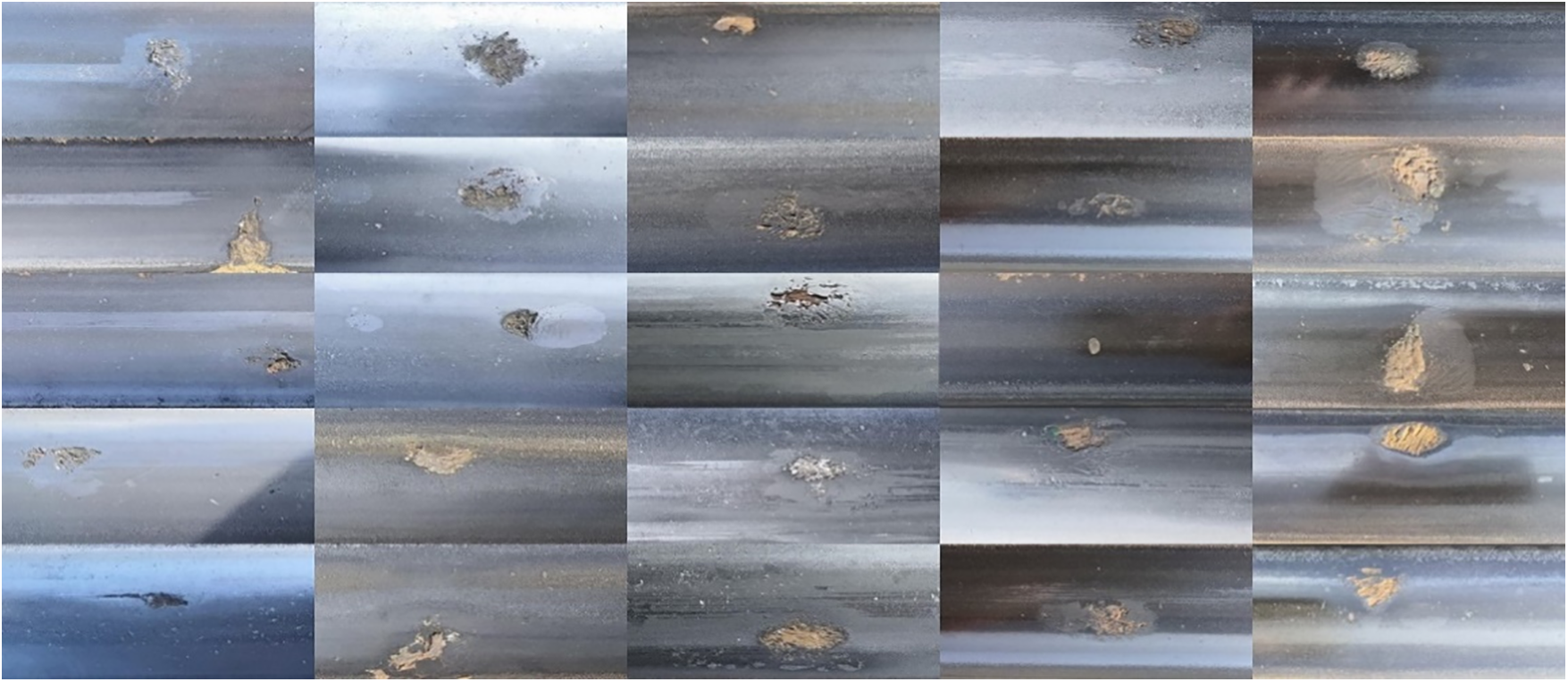
Figure 7: A partial sample of the Rail-BY dataset

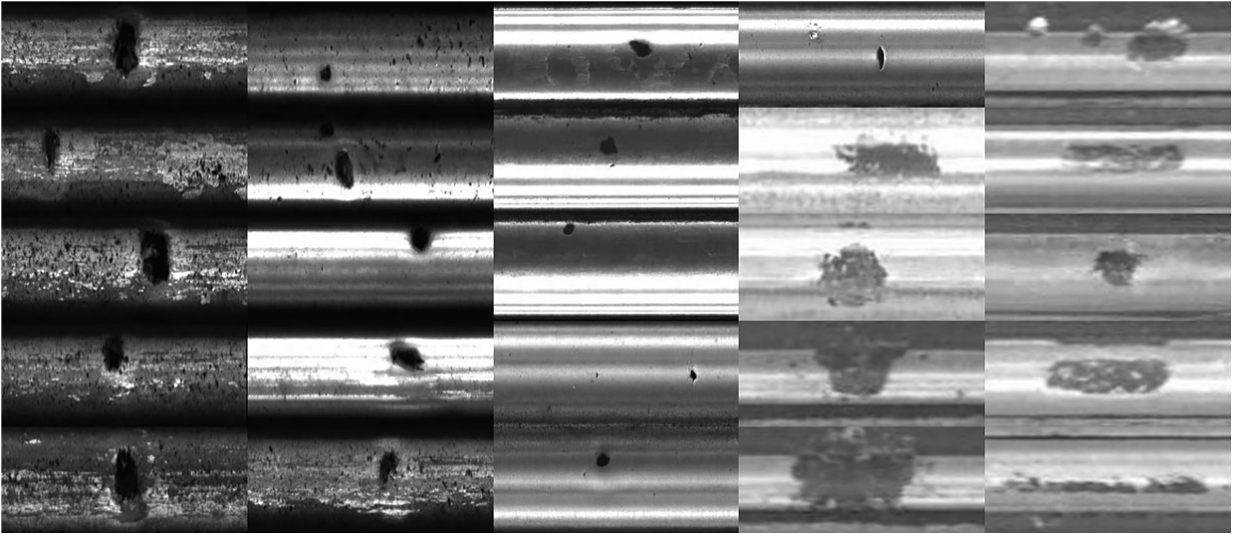
Figure 8: A partial sample of the RSDDs dataset

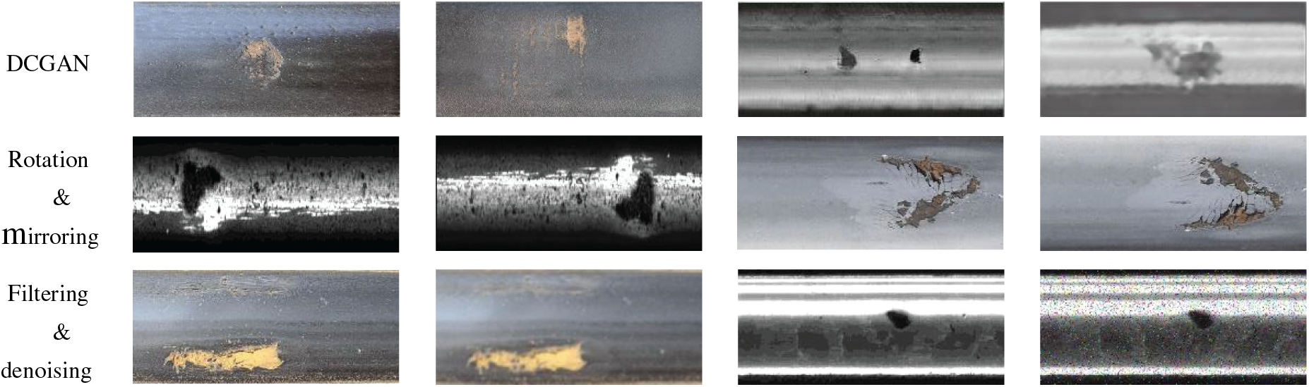
Figure 9: Example of partially expanded samples

For gauging segmentation accuracy, metrics such as PA, IoU, Dice coefficient, and Precision were employed. Additionally, Params and Floating-Point Operations (FLOPs) were harnessed to appraise the magnitude and intricacy of the algorithm. Herein, PA symbolizes the fraction of aptly classified pixels, IoU elucidates the congruence between the prognosticated outcomes and the benchmark, the Dice coefficient quantifies the similitude between anticipated outcomes and the benchmark, and Precision delineates the ratio of pixels identified as defective within the set prognosticated by the segmentation network. An augmentation in these four parameters intimates heightened precision in defect area segmentation. The computations are elucidated in formula (17) through formula (20), where X typifies the anticipated result, and Y signifies the benchmark. Concurrently, Params delineates the aggregate parameter of model training, while FLOPs quantify the tally of floating-point operations. A diminution in Params and FLOPs intimates a reduction in model complexity.

PA=TP+TNTP+TN+FP+FN(17)

IoU=TPTP+FP+FN=|X∩Y||X∪Y|(18)

Dice=2TP2TP+FP+FN=2|X∩Y||X|+|Y|(19)

Precision=TPTP+FP(20)

The apparatuses harnessed for experimentation comprised an Intel Core i9-10920X CPU@3.50 GHz, RAM of 128 GB, dual NVIDIA GeForce RTX 3090 GPU, underpinned by Python 3.8 and PyTorch 1.8.1. During the experiments, a benchmark of 160000 iterations was established, utilizing the AdamW optimizer. Parameters were set at β1 = 0.9, β2 = 0.999, with a learning rate of 0.00006, batch_size of 2, and weight_decay set to 0.01. Loss trajectory for the validation set across the Rail-BY and RSDDs datasets is illustrated in Fig. 10. A stability in training loss post the 160000 iterations indicates an optimal training outcome.

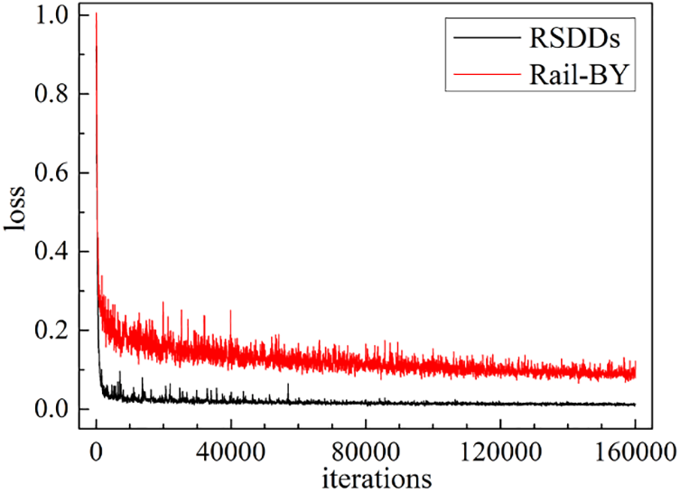
Figure 10: Improved UPerNet validation loss curve on Rail-BY and RSDDs

To ascertain the efficacy of the enhanced methodology presented in this study, a comparative examination of the segmentation outcomes of various modules on the two datasets was performed. Table 1 delineates the segmentation outcomes for diverse modules. The foundational backbone network utilized was ResNet50, with normalization facilitated via BN, and the loss function being the cross-entropy loss function. An examination of Table 1 reveals that solely substituting ResNet50 with Swin-T ameliorated PA, IoU, Dice, and Precision by 8.06%, 11.42%, 7.3%, and 9.52%, respectively on the Rail-BY dataset. Conversely, on the RSDDs dataset, improvements were noted at 3.48% for PA, 4.45% for IoU, 2.59% for Dice, and 1.7% for Precision. A comprehensive enhancement in UPerNet’s segmentation accuracy was observed, with the most pronounced improvement reflected in the original UPerNet. Additionally, the incorporation of Swin-T for feature extraction culminated in a reduction of Params by 6.55 M. The backbone network grounded in the Transformer architecture decidedly surpassed CNN-based networks in terms of performance. The employment of the SyncBN normalization technique and the Lovász-hinge loss function predominantly augmented PA. Given that these don’t pertain to network structure modifications, their impact on network complexity was minimal.

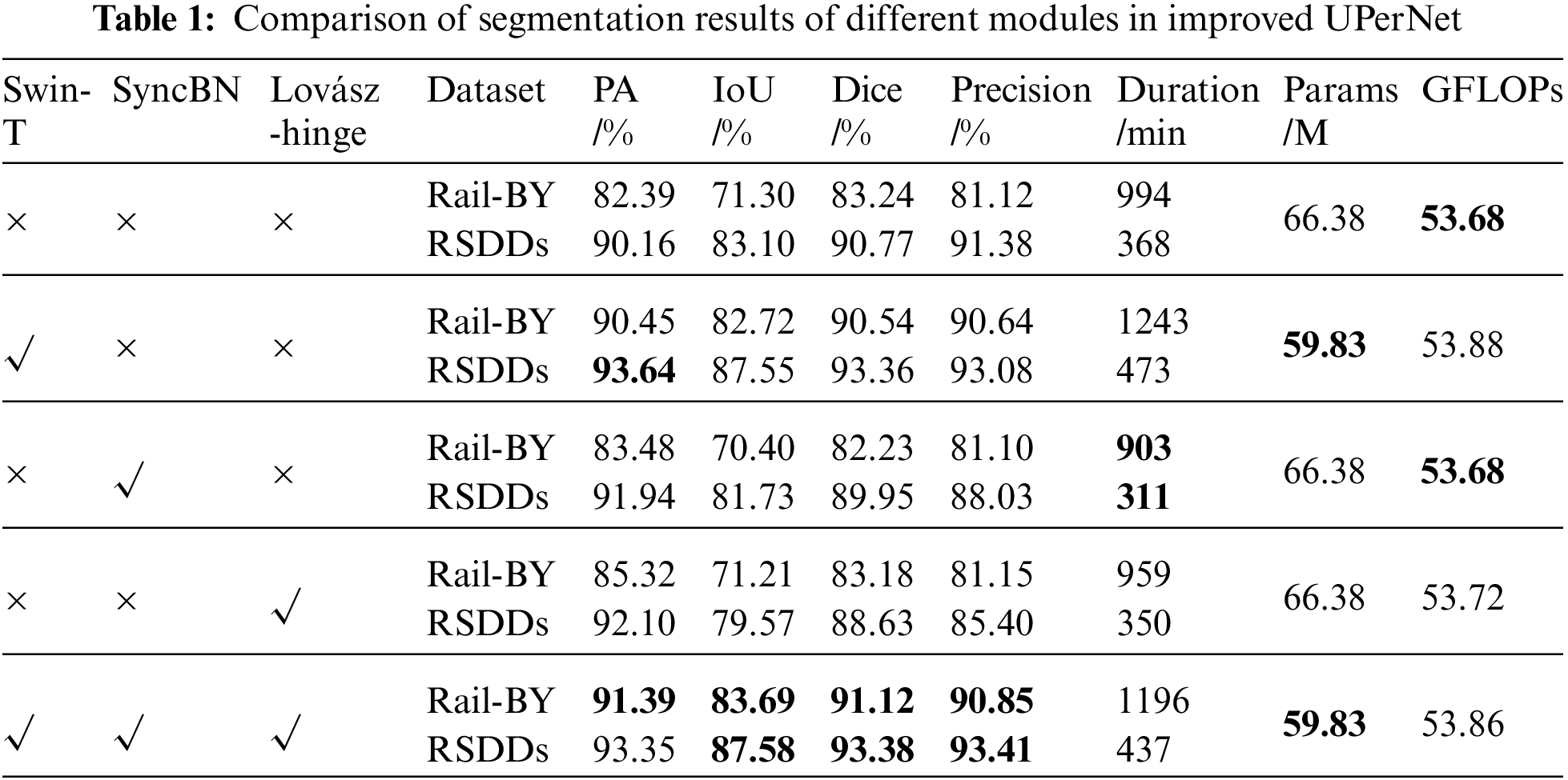
Table 2 presents the training outcomes of the refined UPerNet network juxtaposed against other prevailing semantic segmentation networks across both datasets. The methodology advanced in this study manifested commendable outcomes on both datasets. When pitted against the high-performing DeepLabV3+, the Rail-BY dataset witnessed enhancements of 6.88% in PA, 6.83% in IoU, and 4.2% in Dice. Precision escalated by 1.38%, whereas on the RSDDs dataset, PA surged by 1.13%, IoU by 0.64%, Dice by 0.37%, but Precision experienced a decrement of 0.41%. The original UPerNet network recorded an FPS of 20.1 Hz on the Rail-BY dataset and 20.2 Hz on the RSDDs dataset. However, the FPS of the improved UPerNet on the datasets diminished by 2.2 Hz and 2.3 Hz, respectively, rendering its detection speed performance relatively moderate. Notwithstanding, while the parameter count of the enhanced method presented herein was reduced relative to the original UPerNet model, it remains considerably expansive when compared to other mainstream semantic segmentation techniques. A visual comparison between the methodology advanced in this study and the outcomes from other segmentation networks is portrayed in Fig. 11.

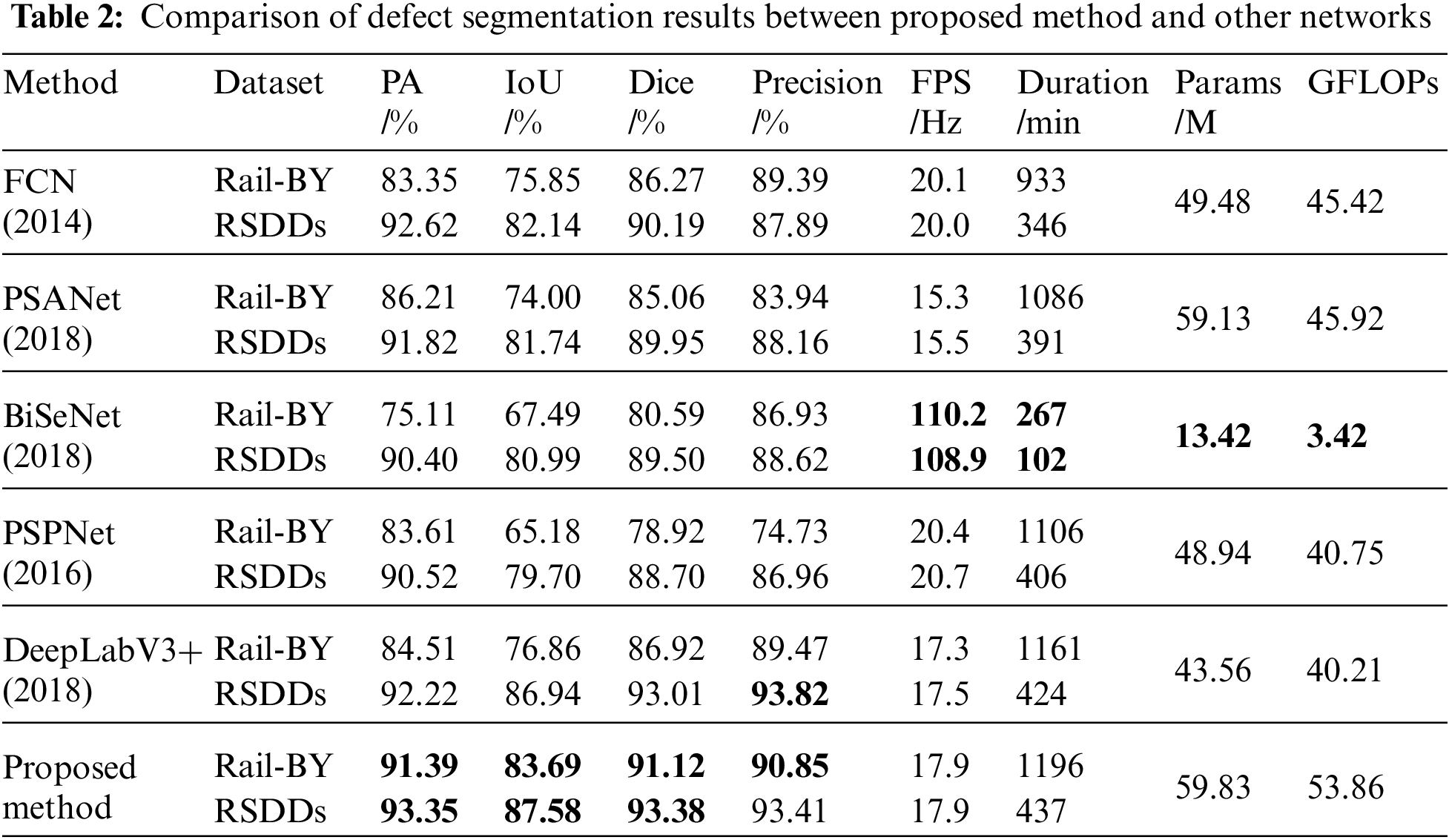
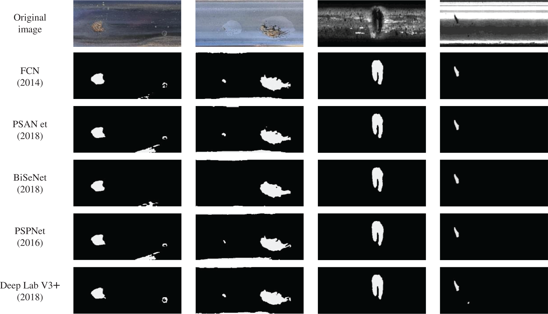
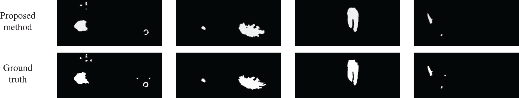
Figure 11: Comparison of visualization results between proposed method and other semantic segmentation methods

5  Defects Parameter Calculation

Deep learning detection algorithms prevalent today are predominantly employed to ascertain the presence of rail defects, yet they seldom incorporate specific parameters associated with these defects. Consequently, in this work, the actual length, width, and area of rail surface defects are computed based on semantic segmentation. Such a computation aids railway maintenance personnel by providing an intuitive comprehension of the exact dimensions of the defects, enabling them to undertake appropriate welding repairs. In the endeavor to calculate the length, width, and area of these defects, distinguishing different defects within the semantic segmentation image is imperative. For this purpose, a method founded on connected component analysis was utilized in this study. As the nomenclature implies, a connected component encompasses interconnected pixels within an image segment characterized by analogous pixel values. By deploying connected component analysis, individual components within an image can be discerned and marked. This technique has garnered considerable traction across various computer vision tasks. However, to obviate any potential interference caused by fluctuations in pixel values when isolating distinct connected components, images are typically subjected to binarization preceding connected component analysis. Integral to this analysis is the determination of neighborhood connectedness. Two predominant criteria for this assessment are the 4-connected neighborhood and the 8-connected neighborhood, the principles of which are delineated in Fig. 12.

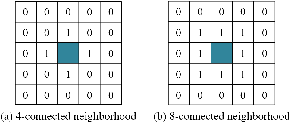
Figure 12: 4-connected neighborhood and 8-connected neighborhood of adjacent pixels

In the realm of the 4-connected neighborhood definition, two pixels can be adjudged as neighboring solely if they exhibit contiguous connections either horizontally or vertically. When point P0(x,y) is examined under the 4-connected neighborhood premise, the coordinates of its four adjacent pixels emerge as P1(x−1,y), P2(x+1,y), P3(x,y−1), and P4(x,y+1). Conversely, under the 8-connected neighborhood paradigm, besides the horizontal and vertical axes, pixels are also deemed interconnected if they adjoin across the diagonal axes. Accordingly, for the point P0(x,y), the eight neighboring pixel coordinates, when evaluated under the 8-connected neighborhood definition, are P1(x−1,y), P2(x+1,y), P3(x,y−1), P4(x,y+1), P5(x−1,y−1), P6(x+1,y−1), P7(x−1,y+1), and P8(x+1,y+1). The methodology outlined in this study harnesses the 8-connected neighborhood definition.

Upon subjecting the rail surface defects to semantic segmentation image analysis using connected components, the OpenCV-Python function cv2. ConnectedComponentsWithStats() is leveraged to discern the connected components. This function yields the count of connected components, the expanse of each individual component, and the dimensions of the encompassing rectangle. The procedural sequence through which defect parameters are derived, rooted in connected component analysis as delineated in this research, is exhibited in Fig. 13.

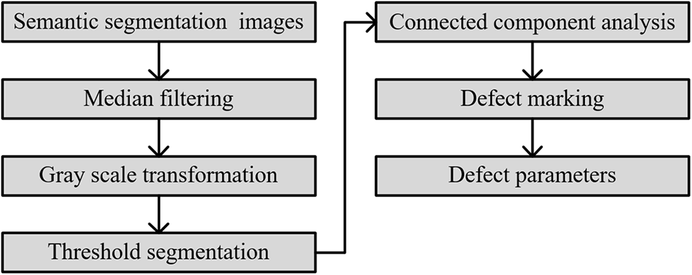
Figure 13: Connected component analysis process of this article

Firstly, the semantic segmentation image, in the initial phase, is subjected to denoising via median filtering. Following this, it undergoes transformation into a binary grayscale image. Subsequent to this transformation, a binary image emerges through threshold segmentation. The concluding step embarks upon connected component analysis. From this analysis, several metrics can be derived: the quantity of connected components within each image, pixel markings within the image, and comprehensive statistics corresponding to each marking—encompassing the length, width, and area of the respective contours. To ensure distinctive identification of different connected components, a colormap facilitates the filling of each with a unique hue. Fig. 14 exhibits the outcomes of this connected component analysis. It is imperative to note that the defect boundaries used within the connected component analysis are devoid of direction. As such, the included analysis does not delve into boundary directionality. Therefore, the graphics leveraged for connected component analysis in this research are undirected, rendering them neither as strongly nor weakly connected graphs.

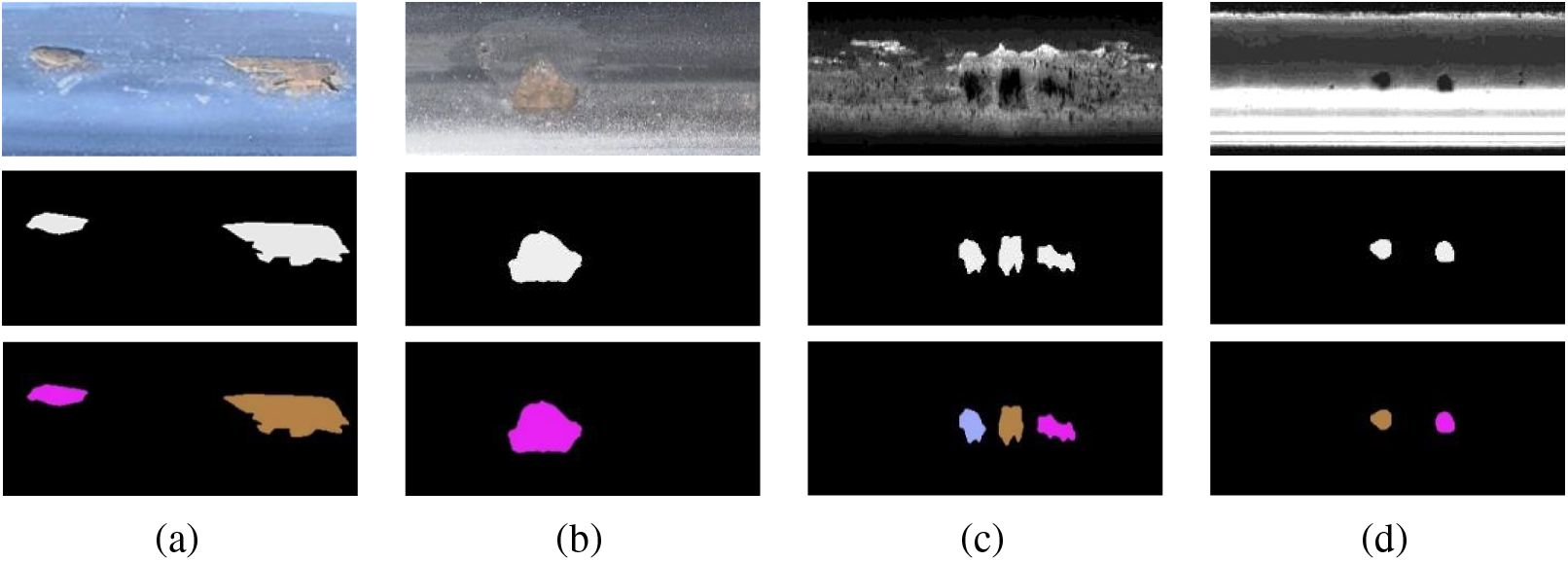
Figure 14: Example of connected component analysis results

The rail head images featured in this study have an actual width of 73 mm, and all utilized rail surface defect images maintain a dimension of 160 × 370 pixels. Leveraging the proportionality principle, the actual length of the rail within the image is discerned to be approximately 168.81 mm. This translates to a total rail area Sentire_real of roughly 12323.31 mm2. formula (21) outlines the calculation methodology for the real rail defect length, drawing upon the ratio between the defect length in the semantic segmentation image Ldefect_seg and the entirety of the image length Lentire_seg. It’s specified that Lentire_real, representing the real rail length within the image, stands at 168.81 mm.

Ldefect_real=Ldefect_seg×Lentire_realLentire_seg(21)

According to the percentage of defect area in the semantic segmentation image Sdetect_seg to the entire image area Sentire_seg, the actual rail defect area Sdefect_real can be calculated, as shown in formula (22), where Sentire_real represents that the actual area of the rail area corresponding to the semantic segmentation image is 12323.31 mm2.

Sdefect_real=Sdefect_seg×Sentire_realSentire_seg(22)

Post connected component analysis, the actual dimensions of the defect within the image—its length, width, and area—can be deduced by incorporating the relevant coefficient. Given that the image’s background pixels too form part of a connected component, any component exceeding an area of 30000 pixels is classified as the backdrop. Fig. 15 presents the algorithm’s operational outcomes. In this depiction, start_x and start_y signify the x and y coordinates of the starting point of the connected component, respectively. Meanwhile, “width” represents its image width, “height” corresponds to its image length, and “area” delineates its space within the image. The terms “actual width”, “actual height”, and “actual area” convey the real-world dimensions of the connected component.

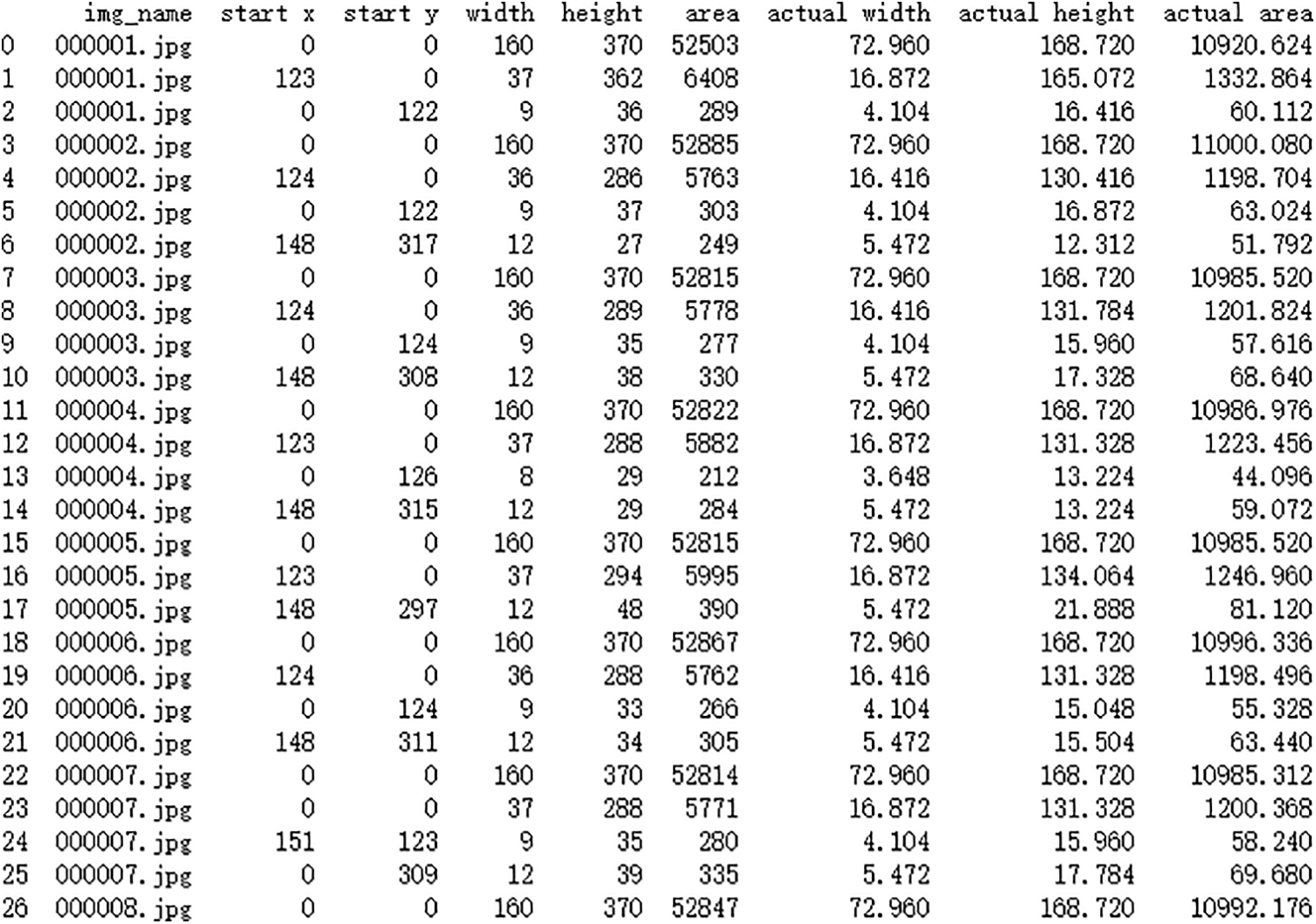
Figure 15: Operating results of damage area parameter calculation

For example, in Fig. 14a, an area, depicted in purple and characterized as connected, was found to be 64 pixels in length and 23 pixels in width, resulting in an area of 960 pixels. When translated to real-world dimensions, the defect exhibited an actual length of 29.18 mm, a width of 10.49 mm, and spanned an area of 199.68 mm2. Additionally, another connected region, colored in coffee, measured 131 pixels in length, 45 pixels in width, and occupied an area of 3803 pixels. Correspondingly, this defect’s actual dimensions were determined to be 59.74 mm in length, 20.52 mm in width, and an area of 791.02 mm2. For Fig. 14b, the analysis revealed a connected area measuring 77 pixels in length, 55 pixels in width, with a total area of 2899 pixels. The actual measurements of this defect were found to be 35.11 mm in length, 25.08 mm in width, and 602.99 mm2 in area. In Fig. 14c, a blue connected area was identified with a length of 28 pixels, a width of 36 pixels, and an overall area of 650 pixels. In actual measurements, the defect was 12.77 mm long, 16.42 mm wide, and spanned an area of 135.20 mm2. A second region, colored in coffee, was 26 pixels in length, 41 pixels in width, and covered an area of 819 pixels. The actual measurements of this defect were 11.86 mm in length, 18.70 mm in width, and an area of 170.35 mm2. A third region, depicted in purple, was found to be 40 pixels long, 28 pixels wide, and had an area of 676 pixels. The real-world measurements of this defect were 18.24 mm in length, 12.77 mm in width, and an area of 140.61 mm2. Fig. 14d showcased a coffee-colored connected area that was 22 pixels long, 21 pixels wide, with an area encompassing 353 pixels. This translated to an actual length of 10.03 mm, a width of 9.58mm, and an area of 73.42 mm2. Another area, colored in purple, had dimensions of 20 pixels in length, 22 pixels in width, and covered 361 pixels. The real-world dimensions of this defect were determined to be 9.12 mm in length, 10.03 mm in width, and 75.09 mm2 in area.

Through the use of connected component analysis, we are able to determine the actual dimensions of the defect, including its length, width, and area. This provides maintenance personnel with a clear and intuitive understanding of the defect’s parameters, enabling them to undertake targeted maintenance actions.

6  Conclusion

In addressing the inefficiencies of conventional machine vision methods and the irregular and intricate defect shapes encountered in rail surface defect detection, an enhanced UPerNet algorithm is presented in this study. Initially, Swin-T is employed as the backbone network to circumvent issues related to inductive bias and the locality of feature extraction inherent in CNN-based backbone networks. Given the influence of BN on the convergence of the semantic segmentation mode, SyncBN is adopted to refine the model, thereby enhancing the training stability during multi-GPU computations. Conclusively, the Lovász-hinge is selected as the loss function to address the challenge posed by cross-entropy loss, which tends to overlook the interdependence between pixels. Experimental findings indicate that the proposed methodology augments detection accuracy across both datasets. Specifically, for the Rail-BY dataset, the PA was recorded at 93.39%, the IoU at 83.69%, the Dice at 91.12%, and the Precision at 90.85%. Similarly, for the RSDDs dataset, the PA, IoU, Dice, and Precision values were determined to be 93.35%, 87.58%, 93.38%, and 93.41%, respectively, illustrating the method’s proficiency in accurately executing rail surface defect segmentation tasks.

Subsequent to the semantic segmentation of rail surface defects, connected component analysis technology is utilized to discern distinct defects within a singular image. Thereafter, by enumerating the pixel count, the authentic length and area of each defect zone are deduced. Such insights prove invaluable for railway maintenance personnel in ascertaining the extent of the inflicted damage.

Acknowledgement: Thanks to our tutors and researchers for their assistance and guidance. The authors also gratefully acknowledge the helpful comments and suggestions of the reviewers, which have improved the presentation.

Funding Statement: This work is supported in part by the National Natural Science Foundation of China (Grant No. 62066024). Gansu Province Higher Education Industry Support Plan (2021CYZC-34),Lanzhou Talent Innovation and Entrepreneurship Project (2021-RC-27,2021-RC-45).

Author Contributions: Study conception and design: Yongzhi Min, Jiafeng Li, Yaxing Li; data collection: Jiafeng Li; analysis and interpretation of results: Yongzhi Min, Jiafeng Li, Yaxing Li; draft manuscript preparation: Jiafeng Li, Yaxing Li. All authors reviewed the results and approved the final version of the manuscript.

Availability of Data and Materials: The data used in this paper can be requested from the corresponding author upon request.

Conflicts of Interest: The authors declare that they have no conflicts of interest to report regarding the present study.

References

1. R. W. Yuan, “Influence of rail head defect on train operation and countermeasures,” Railway Operation Technology, vol. 6, no. 3, pp. 120–121, 2000. [Google Scholar]

2. X. Gibert, V. Patel and R. Chellappa, “Deep multitask learning for railway track inspection,” IEEE Transactions on Intelligent Tranportation Systems, vol. 18, no. 1, pp. 153–164, 2017. [Google Scholar]

3. Q. Y. Li and S. W. Ren, “A real-time visual inspection system for discrete surface defects of rail heads,” IEEE Transactions on Instrumentation and Measurement, vol. 61, no. 8, pp. 2189–2199, 2012. [Google Scholar]

4. L. S. Wu, Y. W. Li, H. W. Chen and L. P. Wan, “Research on rail defects automatic detection technology based on image region partition,” Laser & Infrared, vol. 42, no. 5, pp. 594–599, 2012. [Google Scholar]

5. Z. D. He, Y. N. Wang, J. X. Mao and F. Yin, “Research on inverse P-M diffusion-based rail surface defect detection,” Acta Automatica Sinica, vol. 40, no. 8, pp. 1667–1679, 2014. [Google Scholar]

6. X. C. Yuan, L. S. Wu and H. W. Chen, “Rail image segmentation based on Otsu threshold method,” Optics and Precision Engineering, vol. 24, no. 7, pp. 1772–1781, 2016. [Google Scholar]

7. C. Taştimur, M. Karaköse and E. Akin, “Rail defect detection with real time image processing technique,” in Proc. of INDIN, Poitiers, France, pp. 410–415, 2016. [Google Scholar]

8. O. Yaman, M. Karakose and E. Akin, “A vision-based diagnosis approach for multi rail surface faults using fuzzy classificiation in railways,” in Proc. of ICCSE, Antalya, Turkey, pp. 713–718, 2017. [Google Scholar]

9. M. Nieniewski, “Morphological detection and extraction of rail surface defects,” IEEE Transactions on Instrumentation and Measurement, vol. 69, no. 9, pp. 6870–6879, 2020. [Google Scholar]

10. H. Zhang, X. Jin, Q. M. J. Wu, Y. Wang and Y. Yang, “Automatic visual detection system of railway surface defects with curvature filter and improved gaussian mixture model,” IEEE Transactions on Instrumentation and Measurement, vol. 67, no. 7, pp. 1593–1608, 2018. [Google Scholar]

11. M. J. Xie, F. K. Lv and X. C. Yuan, “Design of rail surface defect detection system based on machine vision,” Journal of Nanchang Institute of Technology, vol. 39, no. 1, pp. 74–79, 2020. [Google Scholar]

12. D. Soukup and R. Huber-Mörk, “Convolutional neural networks for steel surface defect detection from photometric stereo images,” in Proc. of ISVC, Las Vegas, USA, pp. 668–677, 2014. [Google Scholar]

13. S. Faghih-Roohi, H. Siamak, A. Nunez, R. Babuska and B. D. Schutter, “Deep convolutional neural networks for detection of rail surface defects,” in Proc. of IJCNN, Vancouver, Canada, pp. 2584–2589, 2016. [Google Scholar]

14. Z. Liang, H. Zhang, L. Liu, Z. He and K. Zheng, “Defect detection of rail surface with deep convolutional neural networks,” in Proc. of WCICA, Changsha, China, pp. 1317–1322, 2018. [Google Scholar]

15. H. Yuan, H. Chen, S. W. Liu, J. Lin and X. Luo, “A deep convolutional neural network for detection of rail surface defect,” in Proc. of VPPC, Hanio, Vietnam, pp. 1–4, 2019. [Google Scholar]

16. X. T. Jin, Y. N. Wang, H. Zhang, L. Liu, H. Zhong et al., “Deeprail: Automatic visual detection system for railway surface defect using bayesian CNN and attention network,” Acta Automatica Sinica, vol. 45, no. 12, pp. 2312–2327, 2019. [Google Scholar]

17. Z. H. Li, Q. Y. Bai, F. M. Wang and H. R. Liu, “Real-time detection system of rail surface defects based on semantic segmentation,” Computer Engineering and Applications, vol. 57, no. 12, pp. 248–256, 2021. [Google Scholar]

18. H. Luo and G. L. Xu, “Rail surface defect detection based on image enhancement and deep learning,” Journal of Railway Science and Engineering, vol. 18, no. 3, pp. 623–629, 2021. [Google Scholar]

19. H. Luo, J. Li and C. Jia, “Rail surface defect detection based on image enhancement and improved Cascade R-CNN,” Laser & Optoelectronics Progress, vol. 58, no. 22, pp. 1–12, 2021. [Google Scholar]

20. Q. Zhang, B. Wu, Y. H. Shao and Z. X. Ye, “Surface defect detection of rails based on convolutional neural network multi-scale-cross fastflow,” in Proc. of PRAI, Chengdu, China, pp. 405–411, 2022. [Google Scholar]

21. U. Zerbst, K. Mädler and H. Hintze, “Fracture mechanics in railway applications––An overview,” Engineering Fracture Mechanics, vol. 72, no. 2, pp. 163–194, 2005. [Google Scholar]

22. A. Vaswani, N. Shazeer, N. Parmar, J. Uszkoreit, L. Jones et al., “Attention is all you need,” in Proc. of NIPS, Long Beach, USA, pp. 6000–6010, 2017. [Google Scholar]

23. J. Devlin, M. W. Chang, K. Lee and K. Toutanova, “Bert: Pre-training of deep bidirectional transformers for language understanding,” in Proc. of NACAL, Minneapolis, USA, pp. 4171–4186, 2019. [Google Scholar]

24. A. Radford, K. Narasimhan, T. Salimans and I. Sutskever, “Improving language understanding by generative pre-training,” 2018. [Online]. Available: https://www.cs.ubc.ca/~amuham01/LING530/papers/radford2018improving.pdf [Google Scholar]

25. A. Dosovitskiy, L. Beyer, A. Kolesnikov, D. Weissenborn, X. Zhai et al., “An image is worth 16x16 words: Transformers for image recognition at scale,” arXiv preprint arXiv: 2010.11929, 2020. [Google Scholar]

26. N. Carion, F. Massa, G. Synnaeve, N. Usunier, A. Kirillov et al., “End-to-end object detection with transformers,” in Proc. of ECCV, Newcastle, Britain, pp. 213–229, 2020. [Google Scholar]

27. H. Chen, Y. Wang, T. Guo, C. Xu, Y. Deng et al., “Pre-trained image processing transformer,” in Proc. of CVPR, Los Alamitos, USA, pp. 12299–12310, 2021. [Google Scholar]

28. Y. Q. Li, C. Z. Li, R. Q. Liu, W. X. Si, Y. M. Jin et al., “Semi-supervised spatiotemporal transformer networks for semantic segmentation of surgical instrument,” Journal of Software, vol. 33, no. 4, pp. 1501–1515, 2022. [Google Scholar]

29. T. T. Xiao, Y. C. Liu, B. L. Zhou, Y. N. Jiang and J. Sun, “Unified perceptual parsing for scene understanding,” in Proc. of ECCV, Munich, Germany, pp. 418–434, 2018. [Google Scholar]

30. H. Zhao, J. Shi, X. Qi, X. Wang and J. Jia, “Pyramid scene parsing network,” in Proc. of CVPR, Hawaii, USA, pp. 2881–2890, 2017. [Google Scholar]

31. Z. Liu, Y. T. Lin, Y. Cao, H. Hu, Y. Wei et al., “Swin transformer: Hierarchical vision transformer using shifted windows,” in Proc. of ICCV, Montreal, Canada, pp. 10012–10022, 2021. [Google Scholar]

32. G. H. Yu, “Research and implementation of image anomaly detection for power grid equipment based on deep learning,” M.S. dissertation, Beijing University of Posts and Telecommunications, China, 2020. [Google Scholar]

33. S. F. Ji, “Clothing image analysis based on neural network,” M.S. dissertation, Beijing Institute of Fashion Technology, China, 2020. [Google Scholar]

34. M. Berman, A. R. Triki and M. B. Blaschko, “The lovász-softmax loss: A tractable surrogate for the optimization of the intersection-over-union measure in neural networks,” in Proc. of CVPR, Salt Lake City, USA, pp. 4413–4421, 2018. [Google Scholar]

35. P. Y. Yuan, W. Y. Hu, X. Q. Wu, J. F. Chen and H. V. Nguyen, “First arrival picking using U-net with lovász loss and nearest point picking method,” arXiv preprint arXiv: 2104.02805v1, 2021. [Google Scholar]

36. T. Kerola, J. Li, A. Kanehira, Y. Kudo, A. Vallet et al., “Hierarchical lovász embeddings for proposal-free panoptic segmentation,” in Proc. of CVPR, New York City, USA, pp. 14413–14423, 2021. [Google Scholar]

37. J. R. Gan, Q. Y. Li, J. Z. Wang and H. Yu, “A hierarchical extractor-based visual rail surface inspection system,” IEEE Sensors Journal, vol. 17, no. 23, pp. 7935–7944, 2017. [Google Scholar]