Convolution-Based Heterogeneous Activation Facility for Effective Machine Learning of ECG Signals

1  Introduction

It is well known that many diseases affect our health in the human ecosystem. According to World Health Organization [1], there are some shocking statistics: Due to heart-related problems, around 17.9 million people die each year, which accounts for 32% of deaths globally. In this, more than 75% of death occurs in low and middle-income countries like India, Malaysia, Pakistan, Sri Lanka, Thailand, Indonesia, and many more. An Electrocardiogram (ECG) is a non-invasive medical diagnostic device that cardiologists and medical practitioners predominately use to record the heart’s physiological activity throughout time.

The morphological characteristics of the ECG signal are shown in Fig. 1 [2], which are pivotal in heart issue identification. The data from the device may be in a signal or image format, so the consultant can see the heart’s electrical activity and check for irregularity in the interval and any pattern change with morphology. Any changes give information about the severity condition of a particular patient. It should note that since heart-related disorders account for nearly one-third of all fatalities worldwide, accurate diagnosis is crucial.

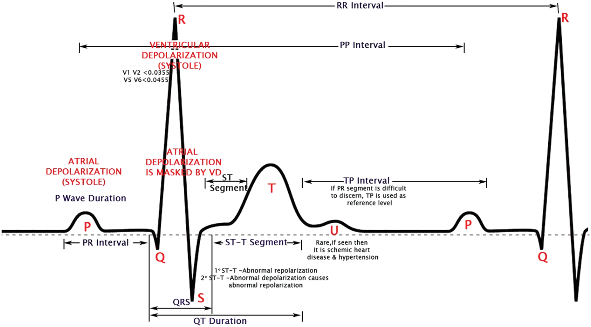
Figure 1: Morphological features of an ECG waveform

In recent years, there has been a rapid advancement in portable ECG monitors for the medical field, including the Holter monitor [3], event monitor, and wearable technology in several healthcare areas. As a result, the growth of the studied ECG data has outpaced the capacity of human cardiologists. Moreover, solid mathematical foundations provide greater accuracy than manual calculation, where Artificial Intelligence (AI) technologies like [2,4,5] come into play. Automation and accuracy in analyzing ECG data has become fascinating recently.

Machine Learning (ML) [6–9] has become increasingly important in various fields due to its many advantages over manual calculations. ML algorithms can process large amounts of data much faster than humans, allowing for more efficient and speedy decision-making. They can also scale to handle large volumes of data and analyze it in real-time, making it possible to analyze data from multiple sources with varying levels of granularity. Additionally, ML algorithms are less prone to errors and can provide consistent results over time, leading to improved accuracy and reliability of data analysis. These algorithms can also detect complex patterns and relationships in data that may be difficult or impossible for humans to see, enabling businesses and organizations to identify new opportunities, optimize processes, and make more informed decisions. Overall, ML has the potential to automate and optimize many aspects of data analysis, saving time and resources, improve accuracy and consistency, and enable more effective decision-making.

Deep Learning (DL) [10–12] techniques are increasingly important in healthcare and medical signal analysis. DL is a subset of ML that uses Neural Networks (NN) to learn from large amounts of data. In medical signal analysis, DL architectures can be trained on vast amounts of medical data to automatically detect patterns and abnormalities that may indicate certain health conditions. DL can help doctors identify patients at high risk of developing a particular state, allowing for early intervention and preventative treatment. DL architectures can also personalize treatment based on a patient’s medical signals, predicting which treatments are most likely effective for a particular patient. DL can improve patient outcomes and reduce the risk of adverse side effects. DL architectures in healthcare and medical signal analysis can significantly improve patient outcomes, reduce healthcare costs, and revolutionize how we diagnose and treat various health conditions.

Convolutional Neural Network (CNN), a typical DL architecture, comprises of multiple layers: convolution layers, pooling layers, and fully connected layers [13–15]. Convolution layers use filters to capture local patterns and features from the input data. Pooling layers down-sample the filtered feature maps and preserving essential features. Max-pooling is widely used in CNNs. A convolution layer with an Activation Function (AF) followed by a pooling layer is termed as a convolutional layer block. In CNNs, there will be several convolution layer blocks followed by a fully connected NN layer. The output of the last convolutional layer block is flattened into a vector representation and fed into fully connected layers for high-level feature extraction. The fully connected layer is the computationally demanding portion of the CNN, and this leads to high execution time.

For biomedical applications such as ECG signal classification, ML algorithms are consistent and reliable for fast decision making (i.e., quick predictions) but they do not match the accuracy levels of DL architectures. Conventional ML algorithms often rely on shallow models with limited ability to learn complicated data patterns. DL architectures on the other hand are highly accurate but time consuming. DL models employ NN with numerous layers that may extract increasingly abstract aspects from data, allowing DL models to learn more complicated data representations, leading to higher performance in many applications. Additionally, DL models can learn directly from raw data, eliminating the need for manual feature engineering that is often required in traditional ML models. To balance these tradeoffs, researchers considered integrating CNN with ML. They focused on combining the computationally less intensive portion of the DL architectures with ML approaches, say for example, combining the convolutional layer blocks of CNN with ML algorithms such as KNN resulting in CNN-KNN [16].

Although the approaches integrating CNN with ML algorithms are faster compared to the baseline CNN approach, these approaches are homogenous in the sense that they use a fixed AFs in the sequence of convolution and pooling layers, thereby limiting the ability to capture unique features. Since various AFs are readily available and each could capture unique features, in this work, we propose a CHAF which uses multiple AFs in the convolution layer blocks, one for each block, with a motivation of extracting features in a better manner to improve the accuracy.

The contributions of this manuscript are as follows:

•   A novel framework for feature extraction, termed as CHAF, is proposed. The CHAF comprises of several convolution layer blocks, each using different AFs. Due to the heterogeneous nature of CHAF, the features are extracted in an efficient manner, thereby give the model a more robust capacity for learning ECG signals.

•   The proposed approach, CHAF-KNN (i.e., CHAF integrated with KNN), is validated on two ECG datasets (PTB dataset and MIT-BIH dataset) and shown to outperform the state-of-the-art approaches. In the case of PTB, CHAF-KNN has an accuracy of 99.55% and an F1 score of 99.68% in just 0.008 s. In the case of MIT-BIT which is relatively larger than PTB, the proposed CHAF-KNN has an accuracy of 99.08% and an F1 score of 98.99% in just 0.07 s.

The remainder of this manuscript is organized as follows. Section 2 reports the survey of different architectures related to ML and DL. In Section 3, we expound on the proposed methodology step-by-step. Section 4 presents the experimental validation of the proposed approach and discusses its advantages and limitations. Finally, Section 5 concludes the paper with recommendations for future research.

2  Literature Survey

The diagnostic analysis of the PTB ECG dataset, a publicly available dataset containing a comprehensive collection of ECG recordings from individuals with diverse cardiac diseases, makes it ideal for different AI algorithmic models. Many ML and DL architectures are performed on the PTB dataset for better accuracy [2]. The KNN algorithm, termed as a lazy learning approach, builds a model by storing feature vectors and class labels from the training dataset. To classify a new data point, KNN calculates distances between the new feature vector and the labeled samples, using Euclidean distance in this case. The K nearest neighbors are identified, and majority voting is employed to assign the new data point to the class label that is most frequent among the K neighbors. Tree-based ML algorithmic models report high accuracy like 97.88% for Random Forest (RF), 98.23% for Extreme Gradient Boosting (XGBoost), and 98.03% for Light Gradient Boosting Machine (LightGBM) and outperform other ML algorithms, and their performance is comparable to the high-end DL architectures [2]. Apart from tree-based algorithms, other ML algorithms like Support Vector Machine (SVM) give better accuracy like 96.67% with morphological & temporal features [17], 98.33% with 220 features [18] & 100% [19], along with grasshopper optimization algorithm, 99.9% for cubic models & 99.8% for a quadratic model [20], 95.1% for Adaptive boosting (AdaBoost) [17] algorithm, and 94.9% for Logistic Regression [21].

CNN architecture [13–15] is an advanced architecture type utilized in DL, especially for image and signal processing tasks. CNNs are one example of advanced architectures in DL, which can refer to any NN architecture that goes beyond the fundamental feed-forward architecture. CNNs are highly suited for tasks like image identification and classification since they automatically learn and detect complicated aspects in the input. Convolutions and pooling operations are frequently used in the architecture of a CNN to extract and compress the most crucial elements from the input data.

Advanced DL architectures can use Recurrent Neural Networks (RNNs), attention mechanisms, and adversarial training, to name just a few. These models are created to address specific issues, such as modeling sequential data, improving model resilience, and providing realistic images or other sorts of data. In general, and particularly for image and signal processing applications, CNNs are a prominent and often-used example of sophisticated DL architectures. However, various cutting-edge designs can be used with varied data or applications.

Regarding DL architecture, the PTB dataset was the subject of relatively few studies, either by using it as a signal or by using images that were transformed from the PTB signal itself. Classification is performed by DL architecture in a few articles [22–25] by converting PTB signals to images; even though by using sophisticated architecture, we can get some good metrics value but still when we do signal-to-image conversation execution time will be more, this will be one disadvantage even if we are using an advanced combination of layers. Researchers directly translated images from the PTB signal in the article [22] without using signal processing procedures and utilized six layers of CNN architecture by removing goldberger-leads or image compression and achieved 81 ± 4% accuracy compared to physicians with 67 ± 7% accuracy. In another scenario, by applying Continuous Wavelet Transform (CWT), the PTB signal is converted to an image by scalogram technique, which is a frequency coefficient of CWT, then classified by simple CNN [25] architecture and got accuracy by 87.50%, followed by 92.50% by Alexnet [26] architecture, applied in parallel to two graphics processing unit, with five convolutional layers, three pooling layers, two fully connected layers, and an output layer, converted to 227 * 227 shape to proceed for classification, 100% by GoogleNet, structured by nine inception layers, then by residual neural network (ResNet) architecture achieved an accuracy of about 99.17% lastly 100% by utilizing EECGNet.

The modelling in the preceding publications is accomplished by transforming signal-to-image. Using the PTB signal, the imbalanced condition can be handled by assigning class weight for Artificial Neural Network (ANN) [23], achieving an accuracy of about 97.64%. The authors of the paper [24] used CNN architecture, in which the predictor network consists of five residual blocks, each with 32 kernels of size 5, for a maximum pooling size of 5, and stride two, followed by 32 neurons fully connected layers activated by ReLU AF, and achieved 95.9% accuracy. Multiple convolution kernels of various receiving domains extract distinctive features of different scales. The retrieved multiple-scale features were combined using CNN and achieved an F1 score of 99.69% [26]. Other DL architectures with long short-term memory and SVM algorithms [27] gained 96.27% accuracy. A scalable framework and transfer learning allow adding more subjects to an existing system without saving previously recorded ECGs [28]. The quantum evolutionary algorithm is used to prune techniques that use the redundant filters in the proposed CNN model, and they have a final accuracy of roughly 99%. As a result, from the studies reviewed, we highlight the metrics values and neglect to take execution time into account, which is another crucial notion. The fact that we are dealing with medical data makes this essential.

DL architectures outperform ML algorithms on average in terms of classification accuracy. In contrast, DL technology demands more processing power. Significant research is being undertaken to utilize a partial CNN architecture for feature extraction. They use various ML algorithms for classification, such as CNN with KNN for plant classification [28], CNN with XGBoost for EEG spectrogram picture analysis [29,30], CNN with SVM for magnetic resonance images [31], weed detection [32], image classification [33], handwritten digit recognition [33,34] and human activity recognition [35]. It is not about the applications they use but about the output. Each technology has advantages and weaknesses; when we combine them, we can achieve something new, in our case, execution time and classification accuracy. Our work offers a computationally efficient classification model for the PTB dataset by integrating computationally less demanding components of DL architectures with ML algorithm (KNN). Some research has been done with the same procedure after converting the signal (1D) to an image (2D). As a result, they achieved an accuracy of 99.52% in the ECG application [36] and an F1 score of 84.19% in the Atrial Fibrillation ECG [36]. Apart from these works, there are many works in literature reporting fast ML models for ECG based heartbeat classification and arrythmia detection [37]. In [38], a comprehensive review of techniques to handle abnormal patterns in ECG signals is presented. Notable among the ECG datasets used in literature for validation of DL and ML algorithms are PTB and MIT-BIH [39–41]. There are many important factors to consider when deciding whether to use DL over ML, and one among them is the AF [42–46]. AFs are essential in DL architecture because they give the model the required non-linearity, which allows it to recognize intricate patterns and connections in the data and also the output of the AF for each neuron in a layer decides whether or not that neuron is activated, and as a result, whether or not its output signal is sent to the neurons in the next layers.

3  Proposed Methodology

It is evident from literature that the approaches integrating CNN with ML algorithms are faster compared to the baseline CNN. However, these approaches are homogenous in the sense that they use a fixed AF in the sequence of convolution layer blocks. In DL architecture, AFs can be used in either a homogeneous manner (i.e., same AF in all layers) [47–49] or a heterogeneous manner (i.e., different AF for each layer). To the best of our knowledge, heterogeneous activation facility is not explored or experimented in literature. Heterogeneous approach can give the model a more robust capacity for learning. Homogeneous approach, on the other hand, might not be as good at encapsulating the complete intricacy of the data. There are several AFs available and the accuracy of the DL approaches vary with the choice of AFs used [42–46]. This reveals the fact that each AF captures features in a manner unique to them. In this section, details of the datasets, significance and choice of AFs, details of evaluation metrics, and the proposed CHAF architecture are discussed in a detail.

3.1 Dataset Description and Implementation

PTB Dataset: Germany’s National Metrology Institute compiled the PTB Diagnostic ECG database [39,40]. Twelve leads, including three frank vectorcardiography leads (vx, vy, and vz), three augmented limb leads (aVR, aVL, and aVF), six precordial leads (V1, V2, V3, V4, V5, V6) and limb leads (I, II, and III) were used to compute each subject’s data. Two hundred ninety distinct participants (209 men and 81 women) contributed 549 data to the collection, 22 of whom lacked a clinical report. A dataset of healthy people (52) and patients with various heart-related disorders (Myocardial Infraction-148, Heart Failure-18, Bundle Branch Block-15, Dysrhythmia-14, Myocardial Hypertrophy-7, Valvular Heart disease-6, Myocarditis-4, Misellaneous-4) is available in the diagnostic groupings for the remaining 268 people.

MIT-BIH Dataset: The MIT-BIH arrhythmia database [40,41] comprises 48 half-hour ECG recordings from 47 subjects, collected between 1975 and 1979. Twenty-three recordings were randomly selected from 4000 24-h ambulatory ECGs from inpatients and outpatients at Boston’s Beth Israel Hospital. The remaining 25 recordings were specifically chosen to include less common but clinically significant arrhythmias not well-represented in a small random sample. The recordings were digitized at 360 samples per second per channel with 11-bit resolution over a 10-mV range. Each record includes computer-readable reference annotations for each beat, with approximately 110,000 annotations in total, independently annotated by two or more cardiologists.

Implementation Details: The PTB diagnostic database and MITBIH dataset can be found at https://www.physionet.org/content/ptbdb/1.0.0/ and https://www.physionet.org/content/mitdb/1.0.0/. The preprocessed signals are obtained as given in [24]. First, the continuous ECG signal is divided into 10-s windows, and one window is selected for analysis. Next, the amplitude values of the selected window are normalized to a range between zero and one. Then, the set of all local maxima is found based on the zero crossings of the first derivative. After that, a threshold of 0.9 is applied to the normalized values of the local maxima to identify the ECG R-peak candidates. The median of the R-R time intervals is calculated as the window’s nominal heartbeat period, say T. A signal segment with a length equal to 1.2 × T is selected for each R-peak. Each selected segment is padded with zeros to reach a predefined fixed length to ensure uniformity. It is important to note that this beat extraction method is both simple and effective in extracting R-R intervals, irrespective of signal morphology [24]. No assumptions are made about the signal’s morphology or spectrum, and all extracted beats have identical lengths, facilitating further processing and analysis. MIT-BIH is a relatively large sized dataset with sample size of 109,444 compared to PTB which has a sample size of 14,550. For our experiments, the train-test split is 70:30. Since the primary focus is on the heterogeneous activation facility, no hyperparameter tuning is introduced. Codes and datasets used for generating the results reported in Sections 3 and 4 are available at https://github.com/anandprems/chaf_tech_science_cmc.

3.2 Convolution Neural Network and Activation Function

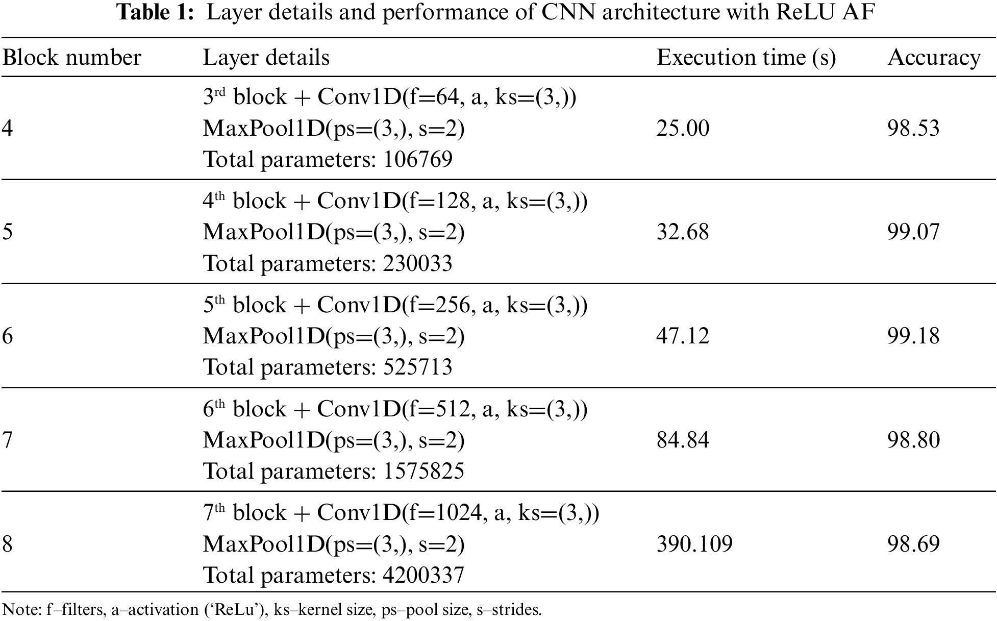
Convolution and pooling layers, which can map and extract features from input data to expedite learning and minimize over-fitting, are unique features of CNN compared to typical neural networks. In the same way, to extract features from the PTB dataset, we use convolution and max-pooling layers, which are considered to be single block throughout the process. Since we were not sure how many blocks would be required to achieve the ideal feature extraction and classification process combination, we initialized with 10 blocks. To boost neurons from one layer to the next, we used ReLU AF in all levels except the output layer, where we used ‘Sigmoid’ AF because our dataset involves binary categorization. In the base level of understanding of CNN architecture, we developed a sequence of blocks consisting of convolution and max-pooling layers employing CNN architecture; since there is no certainty on the best number of blocks to use, we initialized with 10 blocks; the accuracy metrics value increased slightly from 93.34% to 99.18% until the sixth block, after which it began to drop in a steady phase as shown in Table 1. In addition, the number of parameters and execution time from block 1 rapidly increases. It is widely agreed that adding more layers does not guarantee that accuracy would improve further. Instead, there will be a saturation point in every dataset; as a result, for our PTB dataset, 6th block is where we will see the best results.

3.3 Finding Suitable Activation Function

While using sequence of blocks (convolution and max-pooling layers) by using PTB dataset, in the initial experimentation from Table 1, we predicted block 6 which gives best result. So, in the experimentation we have utilized ReLU AF (Homogeneous). Most researchers favour ReLU [46] AF for its functionality while using DL architecture in numerous types of study. In our experimentation, we first used ReLU AF for all the layers, then for the final layer, we used ‘Sigmoid’ AF as the default due to binary categorization. In the next level of experimentation, in order to visualize the significance of AF, we applied different AFs (homogeneously) to the same CNN architecture with six blocks and compared their execution time and accuracy. Among all AFs calculated, for SoftMax AF (in 75.55 s) and Sigmoid AF (in 45.48 s), the performance accuracy is 72.14%, while other AFs like Swish (99.23% in 75.52 s), Exponential Linear Unit (elu) (99.33% in 72.36 s), Parametrized ReLu (99.16% in 77.77 s), Scaled Exponential Linear Unit (selu) (99.04% in 52.84 s), Concatenated ReLu (crelu) (98.92% in 67.36 s), ReLu-6 (99.16% in 66.19 s), Leaky ReLu (99.27% in 68.32 s), ReLu (98.94% in 45.59 s), Tanh (99.46% in 46.91 s), Gaussian Error Linear Unit (99.34% in 54.41 s), Linear function (99.49% in 44.59 s), SoftSign (99.31% in 71.74 s), SoftPlus (96.94% in 71.45 s) and Mish AF (99.55% in 60.26 s), which has overall accuracy of above 95%. It can be inferred from that SoftMax and Sigmoid are insignificant in this case. Therefore, it is wise to exercise greater caution by experimenting with various AFs in order to attain high accuracy and a short execution time.

3.4 Metrics for Model Evaluation

For ML and DL technologies, we need to justify our model by using metrics value. Metrics provide a clear and concise summary of the model’s performance and can aid in developing trust in the model’s outcomes. Metric values enable us to assess how well a model performs on a specific task and identify the areas where the model may be improved. Among many available metrics, confusion matrix based metrics have more significance, as they provide complete knowledge of a model’s performance. The matrix contains information about the model’s True Positive (TP) which denotes the number of correct positive predictions, True Negative (TN) which denotes the number of correct negative predictions, False Positive (FP) which denotes the number of wrong false predictions (i.e., false alarms), and False Negative (FN) which denotes the number of wrong negative predictions. These parameters are in turn used to determine a model’s accuracy and related metrics such as precision, recall, and F1 score.

Accuracy is defined as the fraction of correct predictions and it is mathematically expressed as

Accuracy=TP+TNTP+FP+TN+FN

Precision is defined as the ratio of correct positive predictions to the total positive predictions and it is expressed as

Precision=TPTP+FP

Recall is defined as the ratio of correct positive predictions to the number of actual positives and it is expressed as

Recall=TPTP+FN

The F1 score considers both precision and recall, and it is defined as follows:

F1score=2×Precision×RecallPrecision+Recall

The F1 score from equation is significant because of its capacity to provide a balanced measure of the model’s performance. In particular, it is useful when both precision and recall are to be balanced. In addition to these accuracy related metrics, execution time is also measured and reported as it is very crucial in biomedical applications. In this manuscript, execution time denotes the computation time in Python 3.9.10 running on an AMD Ryzen 7 4800H with Radeon Graphics 2.90 GHz, RAM 16 GB. For certain models or applications, the accuracy will be high at the cost of execution speed. On the other hand, certain models or applications have lesser execution time at the compromise of accuracy. Therefore, for thorough validation of our proposed approach, five metrics are considered: Accuracy, precision, recall, F1 score and execution time.

3.5 Convolution-Based Machine Learning Algorithms

From the second experimentation, with AF, we come to know, not only ReLU AF performs well for our PTB dataset, but by utilizing different AFs in a homogeneously scenario, we got best AFs with good accuracy and also faster process (Execution time). From the experimentation done so far, we have seen, the number of parameters and the complexity of the model rises as the number of layers in CNN architecture increases to certain point but not as exponentially, which leads to greater performance in terms of accuracy to certain block (here till 6th block). However, there comes expense of higher computing time and memory utilization, making the model difficult to apply in real-world applications. As a result, when constructing any DL architecture, including CNN, it is important to balance metrics values, model complexity, and computational performance. While in the case of ML algorithms, it has some advantages over DL architectures, such as being constructed on mathematical models rather than layers, the complexity and computational performance will be better when compared to DL. ML algorithms, such as KNN, SVM, RF, and XGBoost, are frequently used also straightforward and interpretable than DL architectures and can work well for our data kinds of low to moderate complexity problems. The process can also be easier and faster to train than DL architectures and require fewer computer resources. While in DL architectures, such as CNN and RNN, may tackle more complicated issues with greater accuracy and efficiency, particularly when dealing with huge datasets and high-dimensional characteristics, but execution time is longer as we will be using more layers. That is where ML comes to picture, when ML fuses with DL architecture then we can expect better result.

3.6 Proposed CHAF-ML Architecture

We built a customized fully connected CNN architecture at the first level and acquired good accuracy with a longer execution time as the blocks increases with layers and also with homogeneous AF (ReLU). As a result, in the next experimentation we utilized different AFs homogeneously for the same CNN architecture along with ReLU AF and as a result we get different best results with accuracy and execution time. As we selected 6 blocks from CNN architecture (based on accuracy), top 6 AFs for each block we selected for further process. In the next stage of experimentation, we modified our CNN architecture like acquiring feature extraction by CNN and then by removing the dense layer, we included ML algorithms in the classification stage. We witnessed some enhanced accuracy as well as faster execution time when compared to the first stage (CNN architecture). As we are dealing with medical data, for faster response, we implemented CHAF to PTB diagnostic ECG database using a variety of ML algorithms and heterogeneous AFs in each layer for enhanced results as shown in Fig. 2.

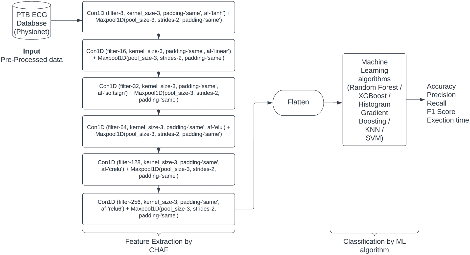
Figure 2: Proposed CHAF-ML architecture

CNNs are powerful feature extractors that can capture spatial and temporal patterns in data. However, they may not always be the most efficient or effective classifiers. By combining CNN with ML algorithms such as SVM, KNN, Decision Tree, and RF, we can leverage the strengths of both approaches to improve classification accuracy. Additionally, utilizing heterogeneous AF between each stage of the CNN can also improve performance. AF plays a critical role in DL architectures, as they introduce non-linearity and enable the model to learn complex relationships between inputs and outputs. However, using the same AF throughout the entire network can lead to a saturation of gradients and slower convergence. By using different AFs at various stages of the network, we can introduce more diversity and flexibility into the model, allowing it to learn more efficiently, and improve the speed of the network. AFs tailored to each layer’s specific characteristics can reduce the required computations, leading to faster execution.

4  Experimental Results and Discussions

In this section, the performance of general CNN-ML architectures and CHAF-ML architectures will be reported and analyzed to decide the number of convolution layers for CHAF and the AFs for the proposed model. Then, the proposed CHAF model will be compared with the baseline CNN model and the state-of-the-art models. The train-test split is 70:30 and the implementation information can be accessed at https://github.com/anandprems/chaf_tech_science_cmc.

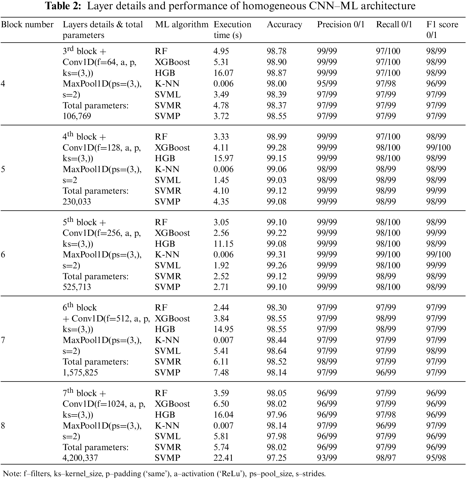
As our domain is related to medical data, apart from accuracy and other metrics, we need to take care of different situations, like how effectively we can create a model with less time consumption; as the medical domain needs some timely advice; sometimes it may lead to collateral damage while diagnosis, so classification layer associated with CNN as in Fig. 2, is placed in a complicated position as layers get increased, so as the complexity, we thought to reduce the complexity in the classification part by replacing dense layer to any ML algorithms. One advantage of ML algorithm over DL architecture is that ML algorithms are built on the mathematical model rather than the layers concept; hence, if you see Tables 2 and 3 compared to Table 1, we can understand the importance of including ML algorithms.

Each block combines convolution and max-pooling layers for the feature extraction process. In Table 1, we utilized CNN architecture with homogeneous AF as ReLU for all the blocks except the classification layer; as our dataset comes under the binary category, we used Sigmoid AF. The accuracy of each block gets increasing from block number 1 to 6; in block 6, we get the best result of 99.18% of accuracy, but parallelly execution time at each block gets increases because of increase in parameters. It is not mandatory if our parameters get increased; our metrics value also will increase, and the complexity level by default, will be more if we have more number parameters. Hence execution time also will get increased. Additionally, accuracy will decrease at one point. After 6 blocks, the accuracy started dropping from 99.18% to 98.69% of 8 blocks, and the execution time also increased to 390.109 s, which we need to avoid for the medical domain. In order to bring novelty, we didn’t perform any new architecture, instead we done some modifications with different stage of experiments. In the first experiment stage, we used CNN with homogeneous AF and found the best block from the combination of convolution and max-pooling will be 6 blocks as from above discussion and from Table 1. Beyond that, if we start concatenating the blocks, the accuracy metric values get dropped because of complexity, and execution time starts increasing. So, in the following experiment stage, we started experimenting with different homogeneous AF; by fixing 6 blocks, we performed with different AFs as discussed in Section 3.3. From the experiment, most of the AFs have accuracy of above 96%. Some AFs, like SoftMax (72.14%) and Sigmoid (72.14%), got less accuracy of about 72%, which is very low and should avoid. So, from this we understand that for different AFs the accuracy and execution time varies and AF is also important factor we need to consider.

In the next stage of experiment, instead of dense layer in CNN for classification process, we modified and utilized ML algorithms like SVM, KNN, RF, Decision Tree, XGBoost and performed with homogenous AF (ReLU) as tabulated in Table 2. So when compared to previous experiment with CNN architecture as in Table 1, here we got better result that also from 6 blocks, it is evident from here, each architecture has some advantage over other, it is not DL which is giving best in all aspects but when we have proper planning we get better result than DL, like we got for RF (99.10% in 3.05 s), XGBoost (99.22% in 2.56 s), Histogram Gradient Boosting (HGB) (99.08% in 11.15 s), KNN (99.31% in 0.006 s), SVM Linear (SVML) (99.26% in 1.92 s), SVM Radial Basis Function (SVMR) (99.12% in 2.52 s) and SVM Polynomial (SVMP) (99.10% in 2.71 s). From the values, we can infer that for the same 6 blocks, compared to Table 1, we get the best result of about 99.31% for CNN-KNN architecture, achieved at 0.006 s, which is very promising by using ReLU homogeneous AF.

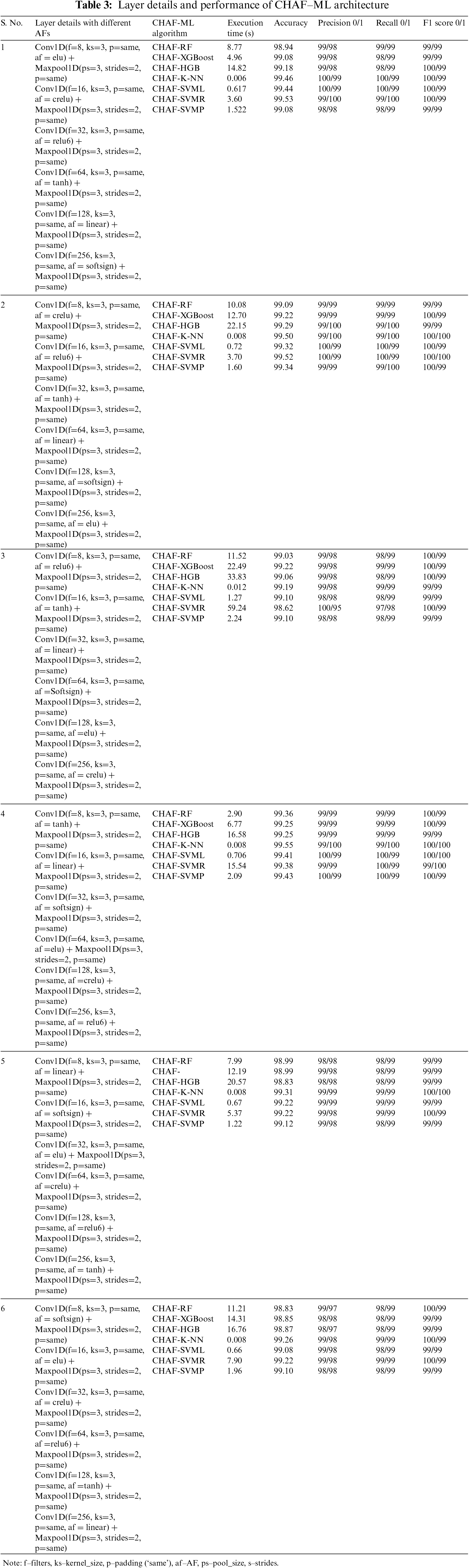
In the last experiment, we performed for CNN architecture with different AFs, fixing the number of blocks as 6, we are again experimenting with different AFs for the same architecture CNN and ML algorithms but this time in a heterogeneous way, which means each layer different AF instead of same. After testing with 16 different AFs, it can be seen by using SoftMax and Sigmoid AF, we are getting very low accuracy, and other AFs are getting the accuracy of the above 92% for all the ML algorithms in combination with CNN feature extraction process. So, from 16 different AFs we experimented, we selected top AFs performing well for the combination of CNN and ML algorithms. CNN-ML best combination of AFs are as elu (RF-98.94% in 9.29 s, XGBoost-98.96% in 12.18 s, HGB-99.10% in 20.18 s, KNN-99.22% in 0.008 s, SVML-99.17% in 0.57 s, SVMR-99.08% in 6.26 s, SVMP-99.08% in 1.20 s), tanh (RF-99.06% in 9.02 s, XGBoost-99.17% in 12.27 s, HGB-99.03% in 20.92 s, KNN-99.45% in 0.004 s, SVML-99.19% in 0.84 s, SVMR-99.26% in 5.94 s, SVMP-99.24% in 1.44 s), linear (RF-99.01% in 13.53 s, XGBoost-99.15% in 15.46 s, HGB-99.12% in 28.55 s, KNN-99.40% in 0.008 s, SVML-99.22% in 0.85 s, SVMR-99.22% in 6.09 s, SVMP-99.33% in 4.33 s), softsign (RF-99.10% in 11.54 s, XGBoost-99.15% in 13.71 s, HGB-99.12% in 22.43 s, KNN-99.42% in 0.012 s, SVML-99.31% in 1.35 s, SVMR-99.49% in 1.35 s, SVMP-99.45% in 3.76 s), crelu (RF-99.22% in 12.49 s, XGBoost-99.19% in 19.53 s, HGB-99.17% in 41.68 s, KNN-99.54% in 0.011 s, SVML-99.26% in 1.03 s, SVMR-98.41% in 40.56 s, SVMP-99.22% in 1.42 s) and relu6 (RF-98.96% in 4.71 s, XGBoost-99.06% in 8.47 s, HGB-99.08% in 18.26 s, KNN-99.24% in 0.008 s, SVML-98.94% in 1.17 s, SVMR-99.28% in 2.51 s, SVMP-99.06% in 1.52 s). From the values itself, we can assume the importance of CNN-ML over CNN architecture in terms of all aspects.

The proposed concept CHAF is another modification we do with the AFs. So instead of using AFs homogeneously, we are utilizing heterogeneous AFs, which means from other AFs, we are selecting the top six AFs because we got the best result in 6 blocks. We implemented different combinations with the selected AFs, and the best combinations are tabulated in Table 3; it is evident that we are getting the best result for the variety of tanh, linear, softsign, elu, crelu and relu6 AFs, so it’s not architecture which gives us best metrics value, we need to consider AFs also, here we get the best result for CHAF KNN-99.55% of accuracy at 0.008 s, then CHAF-SVML-99.41% of accuracy at 0.706 s when compared to DL architecture, the model complexity is lesser for KNN and Linear SVM algorithms, that is why we can achieve best accuracy with faster execution.

To establish comparison with the state-of-the-art, the proposed CHAF-KNN model and three other models are first validated on PTB dataset. The proposed CHAF-KNN model utilizes the CHAF for extraction of features and KNN for classification. The CHAF in this case comprises of six convolution layer blocks, each using different AFs (i.e., tanh, linear, softsign, elu, crelu, relu6). This choice is based on the performance reported in Tables 2 and 3. Three models used for comparison are baseline CNN comprising of six convolution layer blocks using ReLu as AF and a fully connected layer [14], CNN-KNN comprising of six convolution layer blocks using ReLu as AF and KNN [16], CNN-XGBoost comprising of six convolution layer blocks using ReLu as AF and XGBoost [50]. For KNN, the value of K is fixed as 5. To validate the generality of the proposed approach, another dataset, the MIT-BIH dataset, is considered for evaluation. As mentioned in Section 3.1, MIT-BIH is a large sized dataset compared to PTB. Therefore, the performance of the proposed CHAF-KNN model is benchmarked using both PTB and MIT-BIH to have a clear understanding of the generality and scalability of the approach. Implementation-wise, in the case of MIT-BIH dataset, the number of convolution blocks is five for all four models compared and the five AFs in the case of CHAF-KNN are relu6, elu, softsign, crelu, and tanh. This choice is based on the preliminary experiments conducted as in the case of PTB. Table 4 shows the comparison of the proposed approach with the state-of-the-art, for both PTB and MIT-BIH datasets. Fig. 3 shows the performance comparison in terms of accuracy and related metrics for both datasets. Similarly, Fig. 4 shows the execution time comparison for both the datasets.

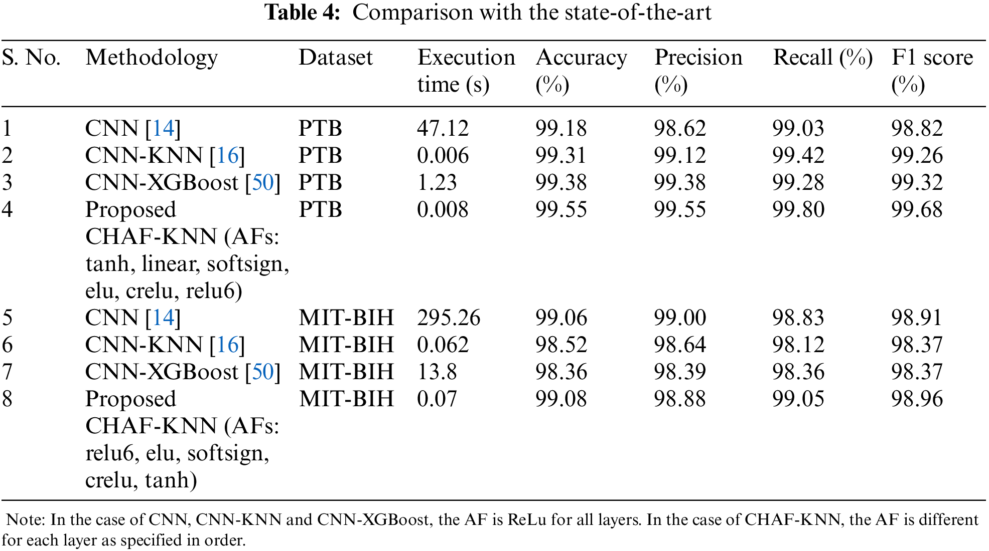
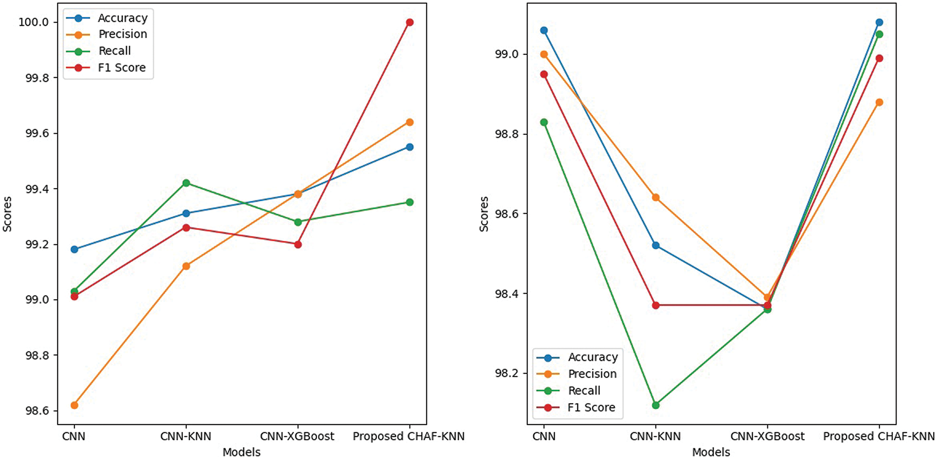
Figure 3: Performance comparison in terms of accuracy, precision, recall and F1 score-for PTB (left) and MIT-BIH dataset (right)

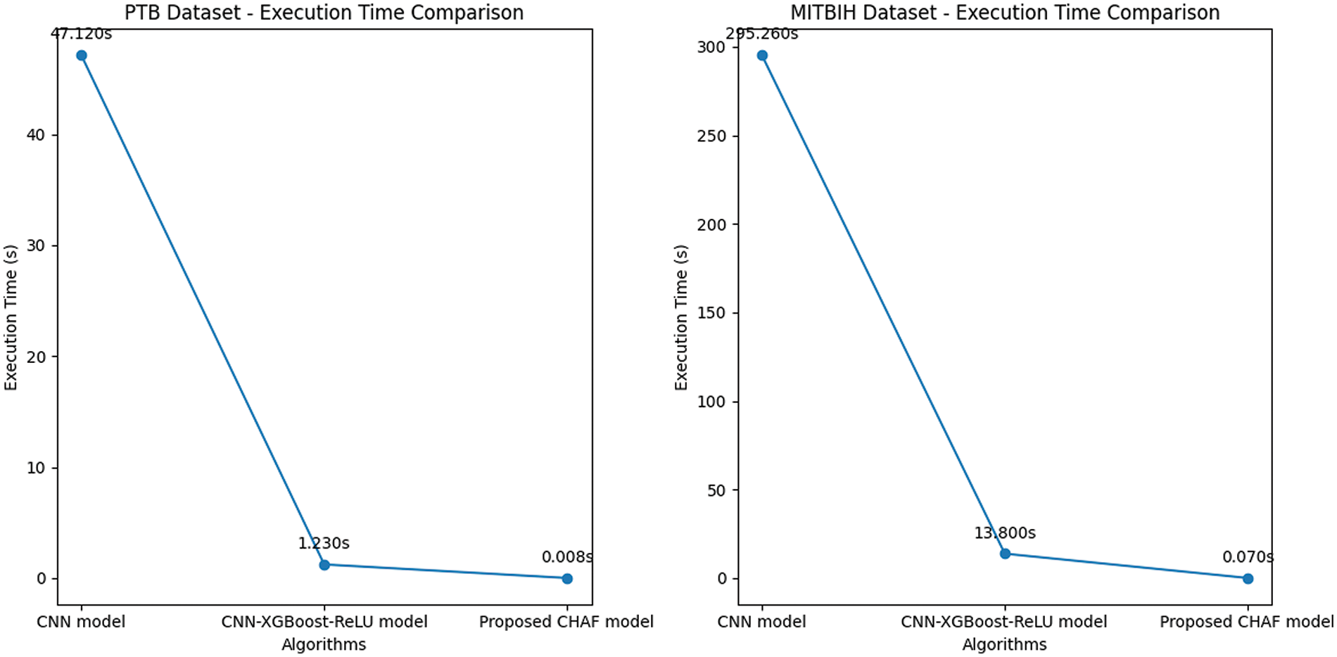
Figure 4: Execution time comparison–PTB (left) and MIT-BIH dataset (right)

In the case of PTB dataset, the proposed CHAF-KNN has an accuracy of 99.55% and an F1 score of 99.68% in 0.008 s, outperforming the state-of-the-art CNN-XGBoost which has an accuracy of 99.38% and an F1 score of 99.32% in 1.23 s. Similarly, in the case of MIT-BIH dataset, proposed CHAF-KNN has an accuracy of 99.08% and an F1 score of 98.99% in just 0.07 s, outperforming the state-of-the-art CNN-XGBoost which has an accuracy of 98.36% and an F1 score of 98.37% in 13.80 s. It can be inferred that, in the proposed CHAF-KNN, the heterogeneous activation facility contributes to improvement in accuracy and F1 score and the KNN expedites the classification process.

Advantages of CHAF Architecture: Architecture-wise, the heterogeneous nature of CHAF introduces more diversity and flexibility into the model. CHAF is accommodative in the sense that it can include multiple AFs and perform well with most ML models. The convolution layer blocks in CHAF utilize different AFs to introduce different non-linearity, thereby enabling the model to learn complex input-output relationships and extract features in a better manner compared to that of the convolution blocks in CNN. This fact is evident from the performance improvement in CHAF-KNN as compared to CNN-KNN, in the case of both PTB and MIT-BIH datasets. As expected, the CHAF-KNN is much faster that the baseline CNN and the CNN-XGBoost, and has speed comparable to that of the CNN-KNN.

Limitations of CHAF and Scope for Improvement: The choice of AFs is based on the results obtained from the preliminary experiments. Therefore, AFs tailored according to each layer’s specific characteristics can be deployed to improve the performance further. On comparing the execution times of the proposed CHAF for PTB and MIT-BIH, it is obvious that the execution time is proportional to the size of the dataset. Special focus on handling scalability is required to bring down the execution time.

5  Conclusion

CNN-ML architectures used a fixed AF in the convolution and pooling layers sequence, making them homogeneous. Due to the availability of a variety of activation functions available, and their capability to capture features uniquely, we proposed a CHAF which uses multiple AFs in the convolution layer blocks, one for each block, with a motivation of extracting features in a better manner. Experimental results presented in this manuscript show that the CHAF is accommodative (i.e., it can accommodate many AFs) and effective with most ML algorithms. For PTB and MIT-BIH datasets, the proposed CHAF-KNN outperforms the state-of-the-art approach, the CNN-XGBoost, with improved accuracy and much lesser execution time. In addition, CHAF-KNN outperforms its homogeneous CNN-KNN with improved accuracy and comparable execution time.

Recommendations for Future Work: (i) Hyperparameter tuning can be introduced to further validate the performance of the proposed approach. (ii) AFs tailored according to each layer’s specific characteristics can be deployed to improve the performance further.

Acknowledgement: The authors would like to express their gratitude to Vellore Institute of Technology (VIT), Chennai, India, for providing valuable support to carry out this work at VIT. We thank Dr. Balasundaram A, Assistant Professor (Senior Grade 2), Centre for Cyber Physical Systems, VIT, Chennai, for his valuable suggestions for the improving the quality of this manuscript.

Funding Statement: The authors received no specific funding for this study.

Author Contributions: Study conception and design: Premanand S, Sathiya Narayanan; data collection: Premanand S; analysis and interpretation of results: Premanand S, Sathiya Narayanan; draft manuscript preparation: Premanand S. All authors reviewed the results and approved the final version of the manuscript.

Availability of Data and Materials: Code formats and datasets used for generating the results reported in Sections 3 and 4 are available at https://github.com/anandprems/chaf_tech_science_cmc.

Conflicts of Interest: The authors declare that they have no conflicts of interest to report regarding the present study.

References

1. World Health Organization on Cardiovascular diseases (CVDs[Online]. Available: https://www.who.int/news-room/fact-sheets/detail/cardiovascular-diseases-(cvds) [Google Scholar]

2. S. Premanand and S. Narayanan, “A tree-based machine learning approach for PTB diagnostic dataset,” in Journal of Physics: Conf. Series, IOP, Publishing, Second Int. Conf. on Robotics, Intelligent Automation and Control Technologies (RIACT 2021), Chennai, India, vol. 2115, pp. 012042, 1–11, 2021. [Google Scholar]

3. G. Nikolic, R. L. Bishop and J. B. Singh, “Sudden death recorded during holter monitoring,” Circulation, vol. 66, no. 1, pp. 218–225, 1982. [Google Scholar] [PubMed]

4. S. Aziz, S. Ahmed and M. S. Alouini, “ECG-based machine-learning algorithms for heartbeat classification,” Scientific Reports, vol. 11, pp. 18738, 1–14, 2021. [Google Scholar]

5. S. Hong, Y. Zhou, J. Shang, C. Xiao and J. Sun, “Opportunities and challenges of deep learning methods for electrocardiogram data: A systematic review,” Computers Biology and Medicine, vol. 122, pp. 103801, 2020. [Google Scholar]

6. M. Javaid, A. Haleem, R. P. Singh, R. Suman and S. Rab, “Significance of machine learning in healthcare: Features, pillars and applications,” International Journal of Intelligent Networks, vol. 3, pp. 58–73, 2022. [Google Scholar]

7. S. M. D. A. C. Jayatilake and G. U. Ganegoda, “Involvement of machine learning tools in healthcare decision making,” Journal of Healthcare Engineering, vol. 2021, pp. 6679512, 1–20, 2021. [Google Scholar]

8. M. Ghassemi, T. Naumann, P. Schulam, A. L. Beam, I. Y. Chen et al., “A review of challenges and opportunities in machine learning for health,” AMIA Joint Summits on Translational Science Proceedings, vol. 2020, pp. 191–200, 2020. [Google Scholar] [PubMed]

9. I. H. Sarker, “Machine learning: Algorithms, real-world applications and research directions,” SN Computer Sceince, vol. 2, pp. 160, 2021. [Google Scholar] [PubMed]

10. D. P. Tobón, M. S. Hossain, G. Muhammad, J. Bilbao and A. E. Saddik, “Deep learning in multimedia healthcare applications: A review,” Multimedia Systems, vol. 28, pp. 1465–1479, 2022. [Google Scholar]

11. D. E. M. Nisar, R. Amin, N. U. H. Shah, M. A. A. Ghamdi, S. H. Almotiri et al., “Healthcare techniques through deep learning: Issues, challenges and opportunities,” IEEE Access, vol. 9, pp. 98523–98541, 2021. [Google Scholar]

12. S. Yang, F. Zhu, X. Ling, Q. Liu and P. Zhao, “Intelligent health care: Applications of deep learning in computational medicine,” Frontier in Genetics, vol. 12, pp. 607471, 2021. [Google Scholar] [PubMed]

13. S. Madhavan and M. T. Jones, “Deep learning architectures, the rise of artificial intelligence,” 2021. [Online]. Available: https://developer.ibm.com/articles/cc-machine-learning-deep-learning-architectures/ [Google Scholar]

14. L. Alzubaidi, J. Zhang, A. J. Humaidi, A. A. Dujaili, Y. Duan et al., “Review of deep learning: Concepts, CNN architectures, challenges, applications, future directions,” Journal of Big Data, vol. 8, no. 1, pp. 53, 2021. [Google Scholar] [PubMed]

15. J. Patterson and A. Gibson, “Chapter 4. Major Architectures of Deep Networks, O’Reilly,” [Online]. Available: https://www.oreilly.com/library/view/deep-learning/9781491924570/ch04.html#convo_neu_net [Google Scholar]

16. S. Ghosh, A. Singh, N. Z. Jhanjhi, M. Masud, S. Aljahdali et al., “SVM and KNN based cnn architectures for plant classification,” Computers, Materials & Continua, vol. 71, no. 3, pp. 4257–4274, 2022. [Google Scholar]

17. W. J. Arenas, S. A. Sotelo, M. L. Zequera, M. Altuve, C. C. González et al., “Morphological and temporal ECG features for myocardial infarction detection using support vector machines,” in G. Díaz, C. C. González, E. L. Leber, H. A. Vélez, N. P. Puente et al. (Eds.CLAIB 2019: VIII Latin American Conf. on Biomedical Engineering and XLII National Conf. on Biomedical Engineering. Cham, Cancún, México: Springer, pp. 172–181, 2019. [Google Scholar]

18. A. K. Dohare, V. Kumar and R. Kumar, “Detection of myocardial infarction in 12 lead ECG using support vector machine,” Applied Soft Computing, vol. 64, pp. 138–147, 2018. [Google Scholar]

19. N. Safdarian, S. Y. D. Nezhad and N. J. Dabanloo, “Detection and classification of myocardial infarction with support vector machine classifier using grasshopper optimization algorithm,” Journal of Medical Signals and Sensors, vol. 11, no. 3, pp. 185–193, 2021. [Google Scholar] [PubMed]

20. M. A. S. B. Goharrizi, A. Teimourpour, M. Falah, K. Hushmandi and M. S. Isfeedvajani, “Multi-lead ECG heartbeat classification of heart disease based on HOG local feature descriptor,” Computer Methods and Programs in Biomedicine Update, vol. 3, pp. 100093, 2023. [Google Scholar]

21. A. Rath, D. Mishra and G. Panda, “Imbalanced ECG signal-based heart disease classification using ensemble machine learning technique,” Frontiers in Big Data, vol. 5, pp. 1021518, 2022. [Google Scholar] [PubMed]

22. H. Makimoto, M. Höckmann, T. Lin, D. Glöckner, S. Gerguri et al., “Performance of a convolutional neural network derived from an ECG database in recognizing myocardial infarction,” Scientific Reports, vol. 10, no. 1, pp. 8445, 2020. [Google Scholar] [PubMed]

23. M. A. Ahamed, K. A. Hasan, K. F. Monowar, N. Mashnoor and M. A. Hossain, “ECG heartbeat classification using ensemble of efficient machine learning approaches on imbalanced datasets,” in 2nd Int. Conf. on Advanced Information and Communication Technology (ICAICT), Dhaka, Bangladesh, pp. 140–145, 2020. [Google Scholar]

24. M. Kachuee, S. Fazeli and M. Sarrafzadeh, “ECG heartbeat classification: A deep transferable representation,” in 2018 IEEE Int. Conf. on Healthcare Informatics (ICHI), New York, NY, USA, pp. 443–444, 2018. [Google Scholar]

25. Y. H. Byeon, S. B. Pan and K. C. Kwak, “Intelligent deep models based on scalograms of electrocardiogram signals for biometrics,” Sensors, vol. 19, no. 4, pp. 935, 2019. [Google Scholar] [PubMed]

26. L. Zheng, M. Zhang, L. Qiu, G. Ma, W. Zhu et al., “A multi-scale convolutional neural network for heartbeat classification,” in 2021 IEEE 20th Int. Conf. on Trust, Security and Privacy in Computing and Communications (TrustCom), Shenyang, China, pp. 1488–1492, 2021. [Google Scholar]

27. P. Khan, P. Ranjan, Y. Singh and S. Kumar, “Warehouse LSTM-SVM-based ECG data classification with mitigated device heterogeneity,” IEEE Transactions on Computational Social Systems, vol. 9, no. 5, pp. 1495–1504, 2022. [Google Scholar]

28. S. C. Wu, S. Y. Wei, C. S. Chang, A. L. Swindlehurst and J. K. Chiu, “A scalable open-set ECG identification system based on compressed CNNs,” IEEE Transactions on Neural Networks and Learning Systems, vol. 34, no. 8, pp. 4966–4980, 2023. [Google Scholar] [PubMed]

29. M. S. Khan, N. Salsabil, M. G. R. Alam, M. A. A. Dewan and M. Z. Uddin, “CNN-XGBoost fusion-based affective state recognition using EEG spectrogram image analysis,” Scientific Reports, vol. 12, pp. 14122, 2022. [Google Scholar] [PubMed]

30. S. Thongsuwan, S. Jaiyen, A. Padcharoen and P. Agarwal, “ConvXGB: A new deep learning model for classification problems based on CNN and XGBoost,” Nuclear Engineering and Technology, vol. 53, no. 2, pp. 522–531, 2021. [Google Scholar]

31. X. Sun, J. Park, K. Kang and J. Hur, “Novel hybrid CNN-SVM model for recognition of functional magnetic resonance images,” in 2017 IEEE Int. Conf. on Systems, Man, and Cybernetics (SMC), Banff, AB, Canada, IEEE Press, pp. 1001–1006, 2017. [Google Scholar]

32. T. Tao and X. Wei, “A hybrid CNN-SVM classifier for weed recognition in winter rape field,” Plant Methods, vol. 18, pp. 29, 2022. [Google Scholar] [PubMed]

33. A. F. Agarap, “An architecture combining convolutional neural network (CNN) and support vector machine (SVM) for image classification,” arXiv: 1712.03541, 2017. [Google Scholar]

34. S. Ahlawat and A. Choudhary, “Hybrid CNN-SVM classifier for handwritten digit recognition,” Procedia Computer Science, vol. 167, pp. 2554–2560, 2020. [Google Scholar]

35. H. Basly, W. Ouarda, F. E. Sayadi, B. Ouni and A. M. Alimi, “CNN-SVM learning approach based human activity recognition,” in El. Moataz, D. Mammass, A. Mansouri, F. Nouboud (Eds.Image and Signal Processing, vol. 12119, pp. 271–281, 2020. [Google Scholar]

36. O. Ozaltin and O. Yeniay, “A novel proposed CNN-SVM architecture for ECG scalograms classification,” Soft Computing, vol. 27, pp. 4639–4658, 2022. [Google Scholar] [PubMed]

37. M. Alfaras, M. C. Soriano and S. Ortín, “A fast machine learning model for ECG-based heartbeat classification and arrhythmia detection,” Frontiers in Physics, vol. 7, pp. 103, 2019. [Google Scholar]

38. R. Jothiramalingam, A. Jude and D. J. Hemanth, “Review of computational techniques for the analysis of abnormal patterns of ECG signal provoked by cardiac disease,” Computer Modeling in Engineering & Sciences, vol. 128, no. 3, pp. 875–906, 2021. [Google Scholar]

39. R. Bousseljot, D. Kreiseler and A. Schnabel, “Nutzung der EKG-signaldatenbank CARDIODAT der PTB über das internet,” Biomedizinische Technik, vol. 40, no. s1, pp. 317–318, 1995. [Google Scholar]

40. A. L. Goldberger, L. A. Amaral, L. Glass, J. M. Hausdorff, P. C. Ivanov et al., “PhysioBank, PhysioToolkit, and PhysioNet: Components of a new research resource for complex physiologic signals,” Circulation, vol. 101, no. 23, pp. e215–e220, 2000. [Google Scholar] [PubMed]

41. G. B. Moody and R. G. Mark, “The impact of the MIT-BIH arrhythmia database,” IEEE Engineering in Medicine and Biology Magazine, vol. 20, no. 3, pp. 45–50, 2001. [Google Scholar] [PubMed]

42. H. Wang, Y. Z. Wang, Y. Q. Lou and Z. L. Song, “The role of activation function in CNN,” in 2020 2nd Int. Conf. on Information Technology and Computer Application (ITCA), Guangzhou, China, pp. 429–432, 2020. [Google Scholar]

43. S. Premanand, “Artificial neural networks–better understanding,” 2021. [Online]. Available: https://www.analyticsvidhya.com/blog/2021/06/artificial-neural-networks-better-understanding/#h2_4 [Google Scholar]

44. P. Baheti, “Activation Functions in Neural Networks [12 Types & Use Cases],” 2021. [Online]. Available: https://www.v7labs.com/blog/neural-networks-activation-functions [Google Scholar]

45. N. S. Chauhan, “An overview of activation functions in deep learning,” 2022. [Online]. Available: https://www.theaidream.com/post/an-overview-of-activation-functions-in-deep-learning [Google Scholar]

46. A. F. Agarap, “Deep learning using rectified linear units (ReLU),” arXiv:1803.08375, pp. 1–7, 2018. [Google Scholar]

47. K. Lakhdari and N. Saeed, “A new vision of a simple 1D convolutional neural networks (1D-CNN) with leaky-ReLU function for ECG abnormalities classification,” Intelligence-Based Medicine, vol. 6, pp. 100080, 2022. [Google Scholar]

48. L. Wang, Y. Mu, J. Zhao, X. Wang and H. Che, “IGRNet: A deep learning model for non-invasive, real-time diagnosis of prediabetes through electrocardiograms,” Sensors, vol. 20, no. 9, pp. 2556, 2020. [Google Scholar] [PubMed]

49. A. J. Prakash, K. K. Patro, S. Samantray, P. Pławiak and M. Hammad, “A deep learning technique for biometric authentication using ECG beat template matching,” Information, vol. 14, no. 2, pp. 65, 2023. [Google Scholar]

50. A. A. Rawi, M. K. Elbashir and A. M. Ahmed, “ECG heartbeat classification using CONVXGB model,” Electronics, vol. 11, no. 15, pp. 2280, 2022. [Google Scholar]