Optimized Deep Learning Approach for Efficient Diabetic Retinopathy Classification Combining VGG16-CNN

1  Introduction

Eye disorders cause different infirmities, such as glaucoma [1], cataracts, DR, and NDR, so early diagnosis and treatment prevent blindness. Glaucoma was expected to affect 64.3 million people worldwide in 2013, rising to 76.0 million in 2020 and 111.8 million in 2040. The diagnosis of glaucoma is frequently put off because it does not manifest symptoms until a relatively advanced state. According to population-level surveys, only 10 to 50 percent of glaucoma patients are conscious that they have the condition. To prevent these diseases, diabetic blood pressure must be kept consistent, and the eye must undergo routine examinations at least twice a year [2]. The second class is Cataracts are one of the most common visual diseases, where the irises appear cloudy. People who suffer from cataracts [3] find problems in reading activities, driving, and recognizing the faces of others. The World Health Organization (WHO) estimates that there are approximately 285 million visually impaired people globally, of whom 39 million are blind, and 246 million have moderate to severe blindness [4]. Better cataract surgery has emerged in recent years than it did in the preceding. In patients without ocular complications like macular degeneration (DR) or glaucoma [5], 85%–90% of cataract surgery patients will have 6–12 best-corrected vision [6]. The third class is DR [7], categorized into two retinal disease cases: proliferative DR (PDR) and non-proliferative DR (NPDR). A low-risk form of DR is called NPDR, where the Blood vessel membranes in the retina are compromised. The retina’s tissues could expand, causing white patches to appear. On the other hand, the high risk, called PDR, High intraocular pressure may cause the blood tissues to have difficulty transferring fluid to the eye, which destroys the cells responsible for transmitting images from the retina to the cerebrum [8]. The fourth class is NDR or typical case.

The paper’s main contributions are distinguished from others by employing data cleansing techniques, TL, and intelligent parameter techniques. Various cleansing techniques are implemented to compare their performance in different applications, involving replacing, modifying, or removing incorrect or coarse data. This enhances data quality by identifying and eliminating errors and inconsistencies, leading to improved learning processes and higher efficiency. Two enhancement filters, auto enhancement (AE) and contrast-limited adaptive histogram equalization (CLAHE), are applied in steps such as augmentation and optimization using adaptive learning rates with different rates for each layer.

This work’s primary contribution lies in analyzing and balancing datasets as a cleansing step to achieve high-quality feature extraction. This is accomplished through the application of AE and CLAHE filters. Subsequently, the VGG16 and CNN algorithms are employed with varying dropout values. Two evaluation stages are conducted: the first measures the performance of cleansed images using a MATLAB program, indicating that AE outperforms CLAHE in metrics. The second evaluation involves training the algorithm and compiling metrics such as AUC, ACC, PRE, REC, confusion matrix (CM), and loss curves, reaffirming the findings of the first evaluation. AE is identified as the superior enhanced filter in this manuscript, achieving metrics not previously obtained with the same database.

The paper is structured as follows: The first section presents related work, followed by an explanation of deep TL, CNN, and the employed cleansing filters with corresponding mathematical equations. Section 3 discusses the VGG16 and CNN algorithms used to divide the original DR images into four groups. Simulation results and visual representations are included. Finally, the paper concludes and outlines potential future work.

2  Related Works

The classification of ophthalmological diseases has been the subject of numerous research proposals. We conducted a literature review to determine the primary methods for glaucoma (GL), cataract (CT), DR, and NDR diagnoses based on images. For a deeper understanding of the issue and to brainstorm workable solutions for raising the ACC of our TL model. We looked at recent journals and publications. After these steps, we reached the goal of using an open-source and freely downloaded dataset(s) and examined a model to compare our efforts with previous experiments. This study introduced an ensemble-based DR system, the CNN in our ensemble (based on VGG16), for different classes of DR tasks. We gained evaluation metrics that are confined in ACC that were achieved with the help of the enhancement filters (98.79% CNN with dropout 0.02 and the used filter auto-enhancement filter with loss 0.0390) and outcomes of CLAHE (96.86% TL without dropout with loss 0.0775). In Ahmed et al.’s research on cataracts, CNN with VGG-19 was applied, where the ACC was 97.47%, with a PRE of 97.47% and a loss of 5.27% [9]. Huang et al. implemented a semi-supervised classification based on two procedures named Graph Convolutional Network (GCN) and CNN, where They scored the best ACC compared to other conventional algorithms with an ACC of 87.86% and a PRE of 87.87% [10]. The Deep Convolutional Neural Network (DCNN) was set up by Gulshan et al. [11] to recognize DR in retinal fundus images, and a deep learning algorithm was applied to develop an algorithm that autonomously detects diabetic macular edema and DR in retinal fundus images. The main decision made by the ophthalmologist team affected the specificity and sensitivity of the algorithm used to determine whether DR was moderate, worse, or both. DCNN, with a vast amount of data in various grades per image, was used to create the algorithm with 96.5% sensitivity and 92.4% specificity. Kashyap et al. [12], using two CNNs, implemented a TL technique. Li et al. [13] created another TL model for categorizing DR into four classes: normal, mild, moderate, and severe. This was in addition to applying TL in two ways while using baseline approaches such as Alex Net, Google Net, VGGNet-16, and VGGNet-19 [14]. The TL model classified the optical coherence tomography (OCT) images for the diseases resulting from the diabetic retina. Kermany et al. [15], who also produced Inception-v3 [16], carried out this novel. Their approach was trained, tested, and validated using OCT images from four different categories: Choroidal Neovascularization, Diabetic macular edema, diabetic drusen, and NORMAL. Additionally, they tested the effectiveness of their strategy using 1,000 randomly chosen training samples from each category. Lu et al. [17] also described the TL technique for diagnosing DR using OCT images. They classified five classes from the OCT data sets [18]. Kamal et al. [19] used five algorithms (standard CNN, VGG19, ResNet50, Dense Net, and Google Net). They concluded that the best metric measurements from the VGG19 algorithms with fine-tuning were 94% AUC. Sensitivity and specificity were 87.01% and 89.01%, respectively. Ahn et al. [20] presented CNN (consisting of three CNVs and Maxpooling in every layer and two fully connected layers in the classifier). The researchers and their colleagues used a private dataset of 1,542 images. They achieved ACC and an AUC of 87.9% and 0.94 on the test data, respectively. The authors in [21–24] used the algorithms (VGG16, VGG16 with augmentation (they used techniques like mirroring and rotating), VGG16 with dropout added to the architecture, and two cascaded VGG16) to get the highest ACC. Pratt et al. [25] added a CNN to this architecture of preprocessing methods for classifying micro-aneurysms, exudates, and hemorrhages on the retina. They fulfilled Sensitivity (95%) and ACC (75%) on 5000 validation images. Islam et al. [26] conducted experiments on eight retinal diseases using CLAHE as a pre-processing step and CNN for feature extraction. Sarki et al. [27] submitted the CNN-based architecture for the dual classification of diabetic eye illness. Diabetic eye disease of several classes’ levels: With VGG16, the maximum ACC for multi-classification is 88.3%, and likewise, for mild multi-classification, it is 85.95%. Raghavendra et al. [28] built a CNN (which included four CNV layers and applied batch normalization, one ReLU, and one Max-pooling at each layer before adding fully connected and Soft-max layers). They can hit an ACC of around 98.13% using 1426 fundus photos from a specific dataset. Recently, presented classification and segmentation approaches for a retinal disease were used to increase the classification ACC. A novel tactic has been posited to boost the fineness of the retinal images (enhancement techniques) before the steps of the classifier. Simulation outcomes for that task reached 84% ACC without fuzzy enhancement, but when applying fuzzy, the ACC reached 100%. This meant that fuzzy was important to discriminate between the different types of retinal diseases [29]. This paper proposed a model for Ocular Disease Intelligent Recognition (ODIR), using augmentation techniques to achieve balance in different datasets. As a result, the ACC of each disease in multi-labeled classification tasks was improved by making better images and working with different TL algorithms [30]. In the paper by Sultan A. Aljahdali, Inception V3, Inception Res-Net V2, Xception, and DenseNet 121 were used as a few examples of pre-trained models that were applied and provided CAD ways of CT diagnosis. The Inception ResNetV2 model had a test ACC of 98.17%, a true positive rate of 97%, and a false positive rate of 100% for detecting eye disease [31]. Nine models (ResNet50, ResNet152, VGG16, VGG19, AlexNet, Google Net, DenseNet20, Inception v3, and Inception v4) served as the foundation for Kamal et al.’s survey paper, which had the best ACC of 0.80. In this article, the dataset is categorized into three ocular illnesses (Strabismus, DR, and GL), where various techniques are used, such as TL, DL, and ML approaches [19]. This review study is based on five retina classes sorted by severity (No DR, Mild, Moderate, Severe, and Proliferate). The distribution of that paper is presented in terms of three model-supervised, self-supervised, and transformer models that achieved percentages of 91%, 67%, and 50%, respectively [32]. Li et al. presented the enhancement methods through two filters. The first filter, Adaptive Histogram Equalization (AHE), enhances the contrast between four classes of images (about 7935 images). The second filter was a nonlocal mean, eliminating the noise. The results of these two filters were used as input measurements of metrics performance: ACC, specificity, and sensitivity (94.25%, 94.22, and 98.11). Consecutively [33], different databases of more than two diseases were used and gave acceptable validation ACC for the training process. This process was checked by five different versions of the AlexNet CNN (Net transfer I, Net transfer II, Net transfer III, Net transfer IV, and Net transfer V): 94.30%, 91.8%, 89.7%, 93.1%, and 92.10% successively [34]. Sharif A. Kamran presented the generative adversarial network (VTGAN). Vision transformers depend on a constructive adversarial network (GAN) made up of transformer encoder blocks for discriminators and generators, as well as residual and spatial feature fusion blocks with numerous losses, to provide brilliant fluorescein angiography images from both normal and abnormal fundus photographs for training. When network metrics were measured on a vision transformer using the three common metrics criteria ACC, sensitivity, and specificity, the scores were 85.7%, 83.3%, and 90%, respectively [35].

3  Materials and Methods

3.1 Data Cleansing (Retinal Image Enhancement)

The diagnosis of DR can be performed manually by an ophthalmologist or through CAD systems. Retinal images are typically captured using a fundus camera. However, several parameters can influence the quality of these diagnostic images, such as eye movements, lighting conditions, and glare. Image quality is critical in the classification, segmentation, and detection processes. Any abnormalities or malformations in the fundus images can have a negative impact on the ACC of the diagnosis. The presence of noise in the images can lead to a decrease in the evaluation metrics used to assess the performance of the diagnostic model. To address these issues, it is crucial to cleanse the datasets of images by removing any malformations or artifacts. The present study uses AE and CLAHE filters to clean data. This cleansing process aims to enhance the images’ quality and improve the diagnostic model’s ACC.

3.1.1 CLAHE

The filter employs a clipping level in the histogram to determine the intensity of the local histogram mapping function. This helps reduce undesired noise in the retinal image [36]. Two essential variables in CLAHE are the block size and clip limit, which are used to adjust the image quality. The clip limit is calculated using the following Eq. (1):

β=MNL⟨(1+α100(Smax−1))⟩(1)

β: the clip limit; Smax: maximum of the new distribution; N: dimensions of the retinal image; L: level of the image; M represents the area size, N represents the grey-level value (256), and represents the clip factor, which expresses the addition of a histogram limit with a value of 1 to 100 [37].

3.1.2 AE Filter

This is the second filter to be used in our proposal. Which increases the brightness overall in the image [38]. It is simply lightness without any light. The luminosity scale is from (0 to 100), where 0 is no light (black), and 100 is white. The arithmetic means of red, green, and blue can be said to be bright. We can recognize the AE function in the MATLAB code by changing the following three parameters to get the highest quality of enhanced images: In the brightness of various objects or areas. Adjust the relative amounts of dark and light regions of Fundus photos using If you increase the contrast, then the light-colored object will be brighter, and the dark-colored object will be darker. You can say it is the difference between the lightest color object and the darkest color object as an arithmetic Eq. (2):

Contrast=luminance differenceaverage luminance(2)

3.2 Enhanced Data Evaluation

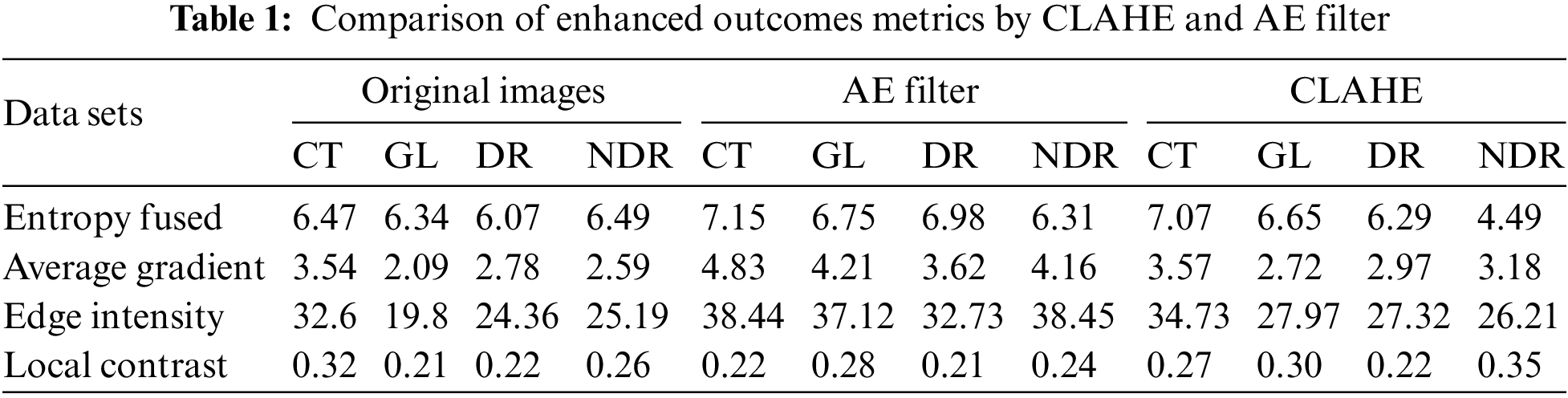
After applying the MATLAB code to enhance the quality of the DR classes using both the CLAHE and AE filters, we conducted further analysis to measure the performance of these filters. A custom MATLAB code function was developed to calculate evaluation metrics based on the outcomes of the filters. Table 1 presents the results of these evaluation measurements, including entropy fused, average gradient, edge intensity, and local contrast. From the table, it can be observed that the AE filter achieved higher values for these metrics compared to the CLAHE filter. The higher values obtained for the evaluation measurements suggest that the AE filter was more successful in improving the quality of the DR classes.

3.3 Convolutional Neural Network

CNNs have recently gained significant popularity, particularly for image classification tasks. These deep learning algorithms utilize learnable weights and biases to analyze fundus images and differentiate between them. CNNs [39,40] have multiple input, output, and hidden layers. They have been successfully applied in various computer vision applications [41], such as semantic segmentation, object detection, and image classification. One notable advantage of CNNs is their ability to recognize essential features in images without human supervision. Additionally, the concept of weight sharing in CNNs contributes to their high ACC in image classification and recognition. CNNs can effectively reduce the number of parameters that must be trained while maintaining performance. However, CNNs do have some limitations. They require a large amount of training data to achieve optimal performance. Furthermore, the training process of CNNs can be time-consuming, especially without a powerful GPU, which can impact their efficiency. CNNs are designed as feed-forward neural networks [42] and incorporate filters and pooling layers for image and video processing [43].

3.3.1 Convolution Layers

CNV layers are the main building blocks of CNN, which include output vectors like a feature map, filters like a feature detector, and input vectors like an image. After going through a CNV layer, the image is abstracted to a feature map, sometimes called an activation map. Convolution occurs in CNNs when two matrices consisting of rows and columns are merged to create a third matrix. This process repeats with an accurate stride (the step for the filter to move). Doing so decreases the system’s parameters, and the calculation is completed more quickly [44]. The output filter size can be calculated as a mathematical Eq. (3). This layer has several results. The first is an increase in dimensionality accompanied by padding, which we can write in the code as “same padding”. The second decreases the dimensionality, and in this process, it happens without padding and is expressed as “valid padding”. Each pixel in the new image differs from the previous one depending on the feature map [45].

Feature Map = Input Image × Feature Detector

F(x)=w−f+2pS+1(3)

W: the size of the Input image, f: the size of the CNV layer filters, p: padding of the output matrix, S: stride.

3.3.2 Activation Function

Activation functions in a CNN model are crucial in determining whether a neuron should be activated based on its input. They use mathematical processes to assess the significance of the information. In the hidden layers of the model, the Rectified Linear Unit (ReLU) activation function is commonly employed. ReLU helps address the vanishing gradients issue by ensuring that the weights do not become extremely small [46]. Compared to other activation functions like tanh and sigmoid, ReLU is computationally less expensive and faster. The main objective of an activation function is to introduce nonlinearity into the output of a neuron. In the suggested framework, the SoftMax function is used for making decisions. Softmax is a straightforward activation function that produces outcomes from 0 to 1, as illustrated in Eq. (4). This activation function is often used for classification tasks [47].

y={xx≥00x>0(4)

Max (0, x); if x is positive, output x, otherwise 0; + ∞ Range: 0 to + ∞.

3.3.3 Pooling Layer

This strategy is applied to reduce the dimensions of the outcomes of previous layers. There are two types of pooling: maximum pooling and average pooling. Max pooling removes the image noise, but average pooling suppresses noise, so max pooling performs better than average pooling [48]. In our model, we introduced max pooling with dropout to prevent overfitting during model training (When a neural network overfits, it excels on training data but fails when exposed to fresh data from the issue domain).

3.3.4 Fully Connected Layer (FC)

The input picture from the preceding layers is flattened and supplied to the FC layer. The flattened vector then proceeds through a few additional FC levels, where the standard processes for mathematical functions happen. The classification process starts to take place at this level. The Soft-max activation function is applied in FC to decide on the classification technique [49].

3.4 Transfer Learning

TL is a crucial component of deep learning [22,50], concentrating on storing information obtained while solving an issue and applying it to other closely related problems. TL increases the effectiveness of new training models by doing away with the requirement for a sizable collection of labeled training data for each new model. Further benefits of TL include faster training times, fewer dataset requirements, and improved performance for classification and segmentation detection problems. VGG16 is the most widely utilized transfer network that we employed in our article (VGG), which proved its effectiveness in many tasks, including image classification and object detection in many different tasks. It was based on a study of how to make these networks deeper.

3.5 Implemented Data Sets

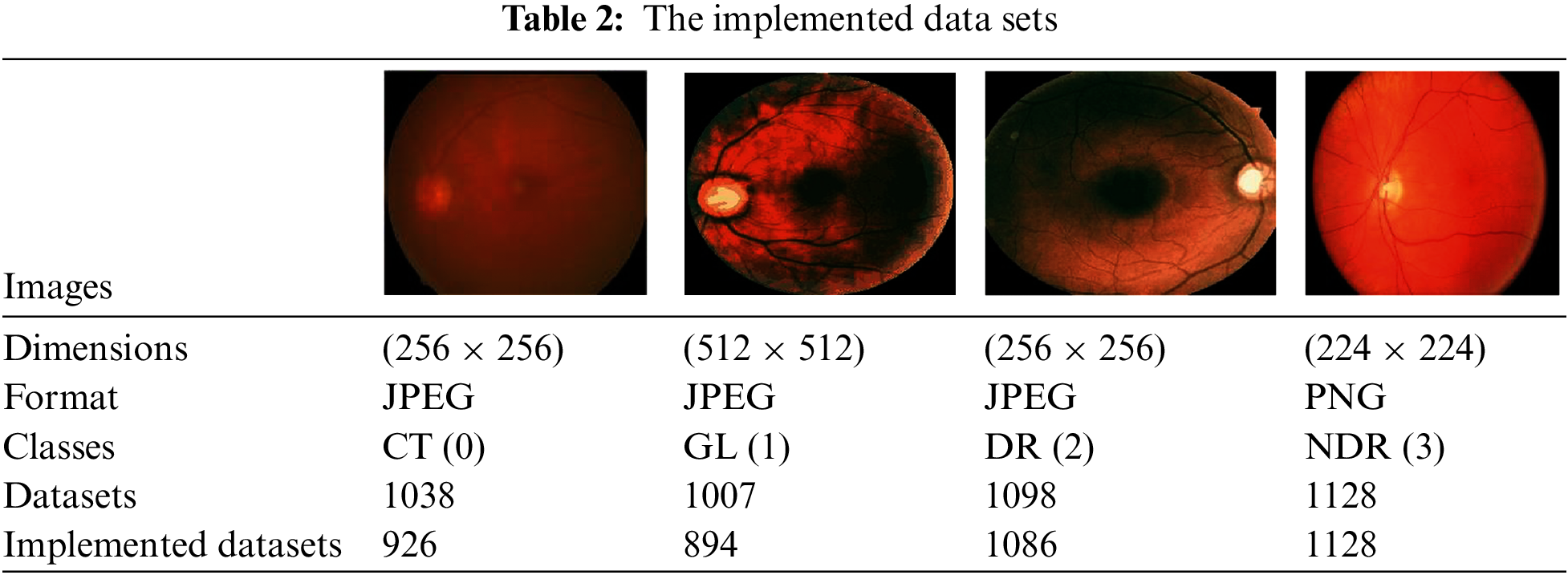
Our proposal utilized datasets divided into four categories: C, GL DR, and NDR. These datasets, consisting of 4271 images, were obtained from the Kaggle dataset [51]. The images in the dataset are in colored format, red, green, blue (RGB), include both left- and right-eye images. The purpose of using these datasets was to classify the images into the categories mentioned above, and the distribution of the images among the classes is summarized in Table 2.

3.6 The Proposed Algorithm of TL and CNN Architecture

The algorithm used is the VGG16 model; the current work suggests modifying the VGG [52,53] model to get better outcomes and achieve better results. In VGG16, only the ImageNet dataset was used for pre-training the model. VGG16 has fixed input tensor dimensions of 224 × 224 with RGB channels. This model is passed through many convolutional neural networks (CNV) layers, where the most miniature used filters were 3 × 3. The most important thing that distinguishes the algorithm of TL is that it does not need many hyperparameters. They used 3 × 3 CNV layers with stride one and Maxpooling (2 × 2) with stride 2. They consistently employed the same padding. Convolution and Maxpooling are organized in the model with block-CNV layers having 64 filters, block-2 CNV layers having 128 filters, block-3 CNV layers having 256 filters, block-4 CNV, and block-5 CNV5 having 512 filters. This task starts with identifying the input RGB images, whose dimensions are 224 × 224, but the images in the database have different sizes. 256 × 256 for CT with a size of 8.84 KB, DR with 46.9 KB, GL with 10.5 KB, and 224 × 224 with a size of 63.8 KB for NDR. The VGG16 models were scaled down to 200 × 200 pixels. The four classes of datasets were used to perform classification procedures by CNN models based on deep VGG16. To prepare for the classification, we should balance the datasets into groups of approximately 1000 for four classes to prevent overfitting or underfitting. After balancing the data, two enhancement filters—the AE filter and the CLAHE filter—performed data cleansing steps. Data cleansing removes noise from original images using a MATLAB program after enhancing, resizing, and reshaping the original images. Image resizing is a necessary process because of the scale difference between images. The image augmentation approach increases the training dataset’s size and improves the model’s capacity. Augmentation in this algorithm occurs in preprocessing datasets; various augmentation process types are used in three steps: Zoom range = 0.15, rotation range = 20, and fill_mode = nearest [54]. The augmentation procedure aims to prevent or minimize overfitting on a small quantity of data [55].

The first model used CNN with a dropout of 0.02 and without TL, which helped improve the classification network and prevent overfitting [56]. A common problem occurs when training data in CNN is insufficient; this technique is presented in [57]. The second is CNN. The third is CNN, with a dropout of 0.2. These three architectures apply in both cases of data division (80%, 20%) and (90%, 10%). It is the same for VGG16; these three cases apply to our model. For the training process, Adaptive Moment Estimation (Adam optimizer) gives the highest results [58], in which the network parameters were optimized. Compared to other optimizers, Descent with Momentum and Root Mean Square Propagation (SGDM and MSPROP) in terms of ACC and loss, Adam is the best optimizer presented in [59]. Datasets were used for training in this scenario with the following parameters: training epoch of 20, batch size of 32, and learning rate (set by the Adam optimizer according to a model designed and changed automatically in the program to fit the training model). Loss in the form of categorical cross entropy; these parameters are shown in Table 3. The final process is to classify the test data and predict the output. Classes initialize the VGG16 fit model and extract the model’s statistical evaluations, such as the CM, ACC, PRE, REC, AUC, and test loss. The block diagram of the proposed algorithm is introduced in Fig. 1.

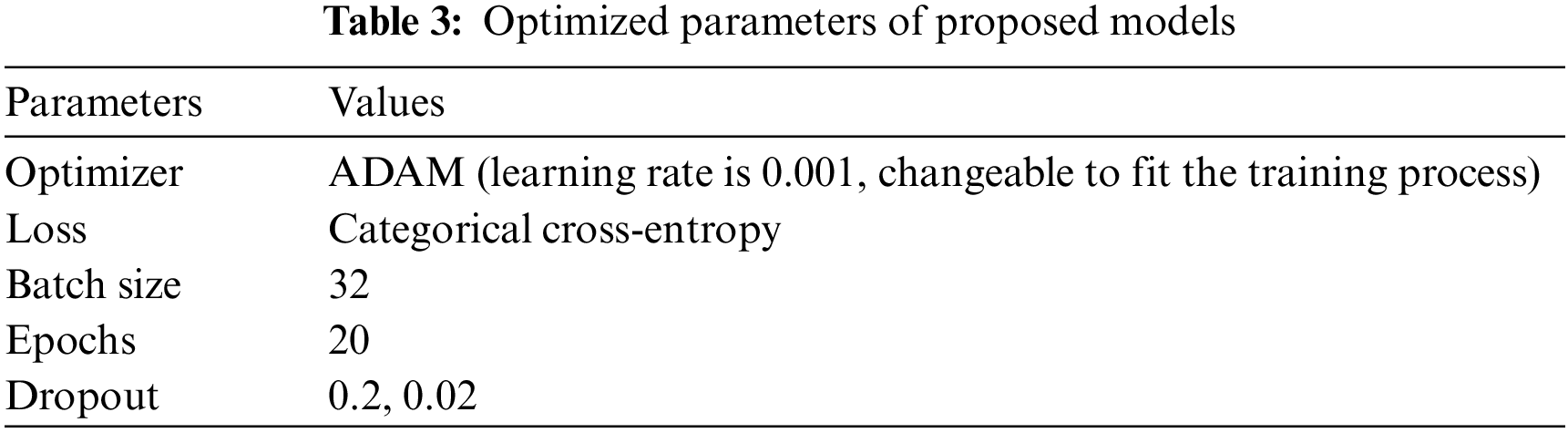
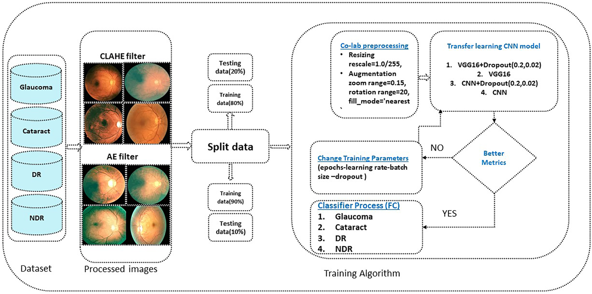
Figure 1: The proposed algorithm

3.7 Evaluation Metrics

According to our models, we observed that the AE filter had excellent ACC, and the incorrectly categorized instances for every class were small. The metrics evaluation depends on four essential measurements ACC, PRE, REC, and AUC. We want to accomplish these objectives with our methodology; however, false predictions must be avoided. Our study’s measurement performance can benefit from the CM because it makes it easy to compare the values of four indexes: True Positive (TP), True Negative (TN), False Positive (FP), and False Negative (FN) [60].

•   True Positive (TP): When the predicted value and actual value are the same and the predicted values are positive, the expected model values are also positive.

•   True Negative (TN): The expected and actual values are identical; besides the real value is negative, the model’s predicted value is negative.

•   False Positive (FP): The predicted value is false; the actual value is negative, and the model’s expected value is positive.

•   False Negative (FN): The predicted value is false; the actual value is positive, and the model’s expected value is negative.

ACC plays a pivotal role in evaluating the metrics; it is the ratio of the sum of true positives and true negatives to the total number of samples. It can be determined from the following Eq. (5):

ACC=TP+TNTP+TN+FP+FN(5)

PRE is the total number of positive predictions (total number of true positives) divided by the total number of expected positives of class values (total number of true positives and false positives). Eq. (6) serves as an example of this.

PRE=TPTP+FP(6)

REC is the number of True Positives (TP) divided by the number of True Positives and False Negatives (FN), and another name for REC is sensitivity. It can be measured from the arithmetic Eq. (7):

REC=TPTP+FN(7)

4  Results and Simulation Graphs

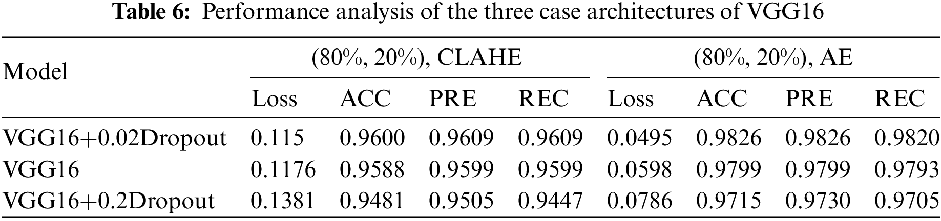
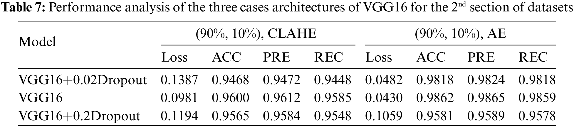
This section examines how well the classification model works by looking at how CNN and VGG16 work when the training parameters for intelligence are changed. We evaluated the results of the model using the Kaggle dataset. The implementation utilized Tensor Flow and Keras, with Keras serving as a deep machine learning package and Tensor Flow acting as the backend for machine learning operations. A CNN model was employed for classification experiments. The model consisted of four CNV layers followed by a max-pooling process. Additionally, for the fully connected layer, the original Dense layers are removed and replaced with two Dense Layers, two with 1024 nodes, and the final one with 4 for classification. The ReLU was applied to all layers. The experiments were conducted in two scenarios: with or without dropouts. In addition, the change in the enhanced dataset division Tables 4 and 5 illustrate the metrics outcomes for CNN models, and Fig. 2 illustrates CNN architecture. The formation of the VGG16 architecture is five blocks of 3 × 3 convolutions, followed by a max pool layer used during the training phase. To further mitigate overfitting, a dropout of 0.2 and 0.02 was applied to the output of the last block. Dropout is a regularization technique that randomly sets a fraction of the input units to zero during training, which helps prevent over-fitting on specific features. After the dropout layer, a dense layer consisting of 1024 neurons was added. The dense layer is fully connected, allowing for more complex interactions between the features extracted by the convolutional layers. Finally, the output layer is dense with four outputs, each corresponding to a specific category of the DR images. This configuration enables the model to classify input images into DR categories. This algorithm is illustrated in Fig. 3, and the results are in Tables 6 and 7.

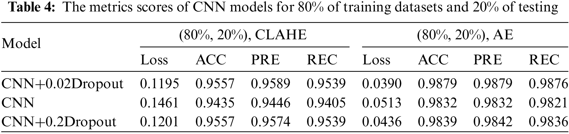
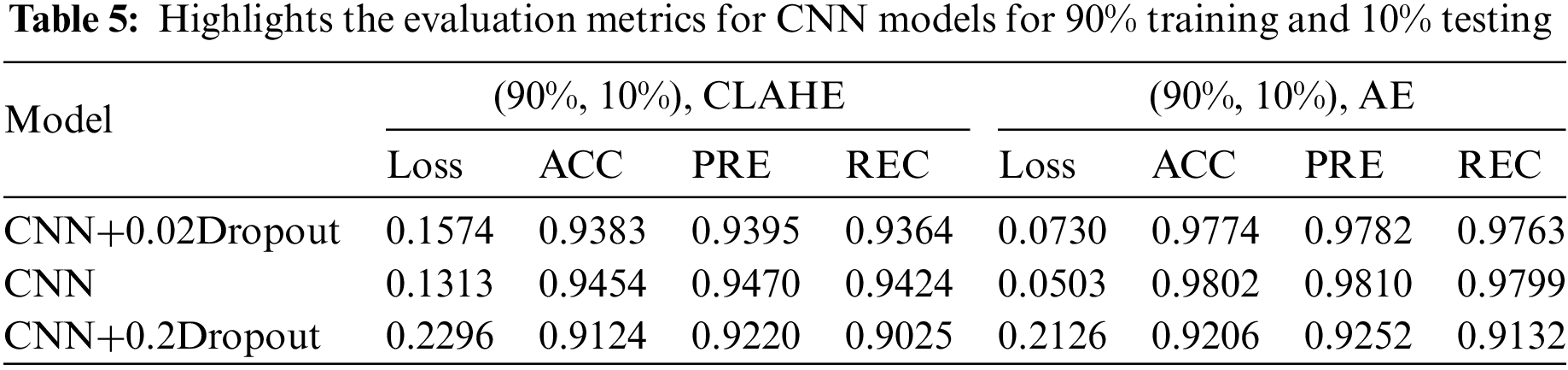
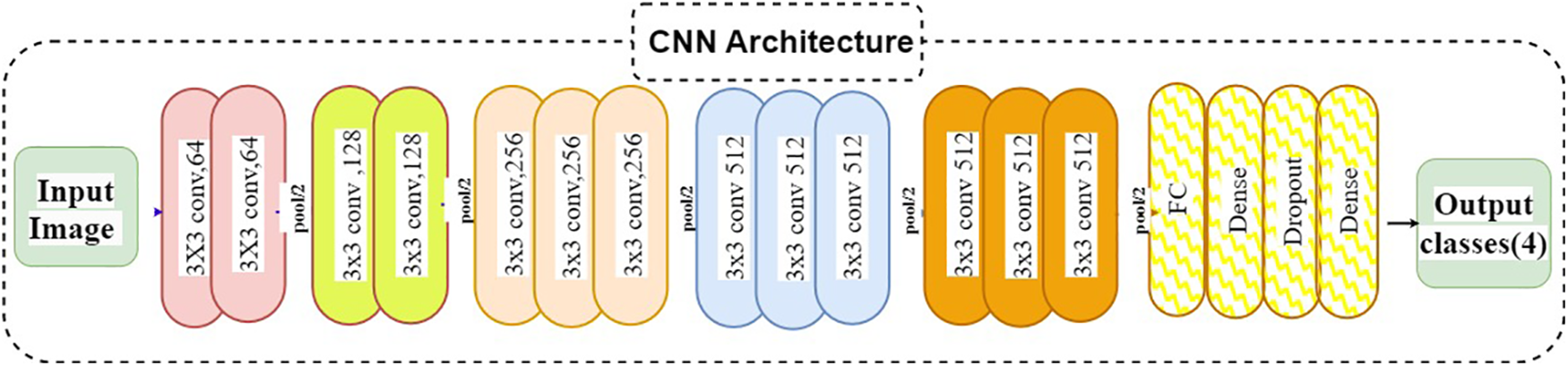
Figure 2: CNN architecture

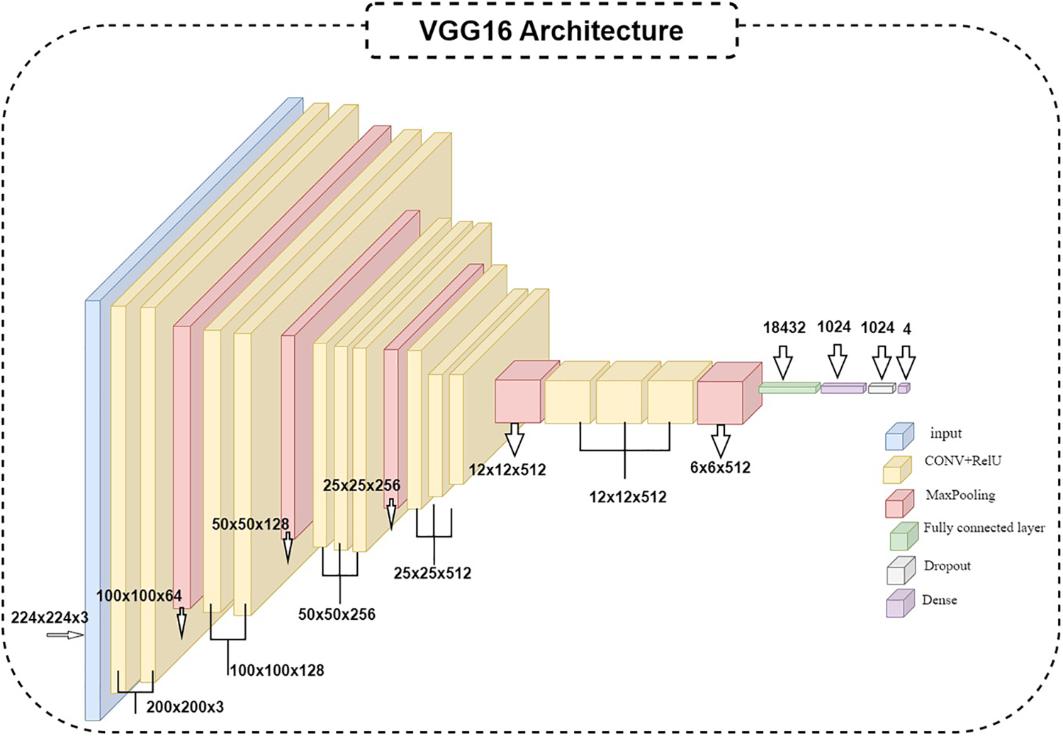
Figure 3: VGG16 architecture

4.1 Concluded Results

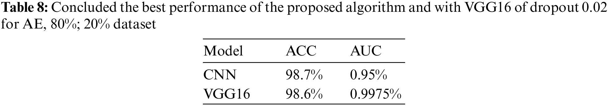
After analyzing different cases of CNN architecture and VGG16, it was observed that the results obtained using the AE filter were the most favorable in terms of metrics. Table 8 presents the ACC of 98.7% achieved when employing the AE filter.

4.2 CM

The enhanced database with the AE filter exhibited the highest performance improvement among the cases studied. Furthermore, the CM in Fig. 4 and the AUC in the figure provided additional insights into the classification outcomes.

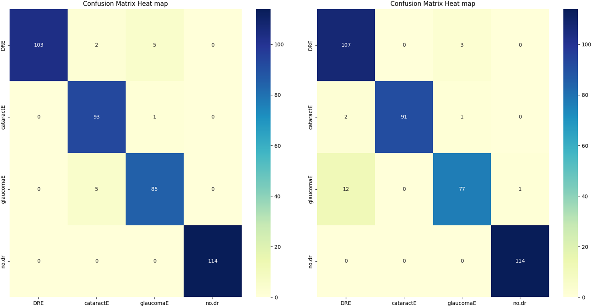
Figure 4: CM of the proposed algorithms

4.3 Receiver Operating Characteristic (ROC) Curve

Plotting the ROC Curve is a trustworthy way to evaluate a classifier’s classification ACC. The True Positive Rate (TPR) and False Positive Rate (FPR) charts allow us to observe how the classifier responds to various thresholds. The closer the ROC curve comes to touching the upper left corner of the picture, the better the model performs in categorizing the data. We may compute the AUC, which shows how much of the graphic is below the curve [61,62]. The model becomes more accurate as the AUC approaches the value of 1. The figure below shows the combined dataset’s AUC score and ROC curve after being tested on four classes of DR. The black, diagonally dashed line shows the 50% area. According to the graphic, the combined model with the VGG16 and CNN of AE filters and AUC performs better at classifying DR and typical retinal pictures. VGG16CNN has AUC curves, as shown in the below Fig. 5.

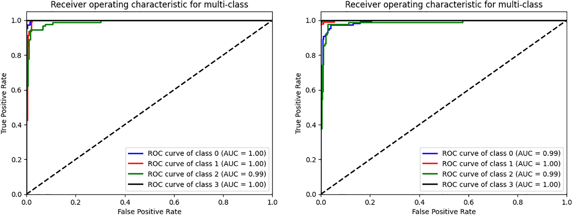
Figure 5: The ROC curve of the VGG16 and CNN evaluated on four datasets. (0) CT, (1) GL, (2) DR, (3) NDR

4.4 Comparisons

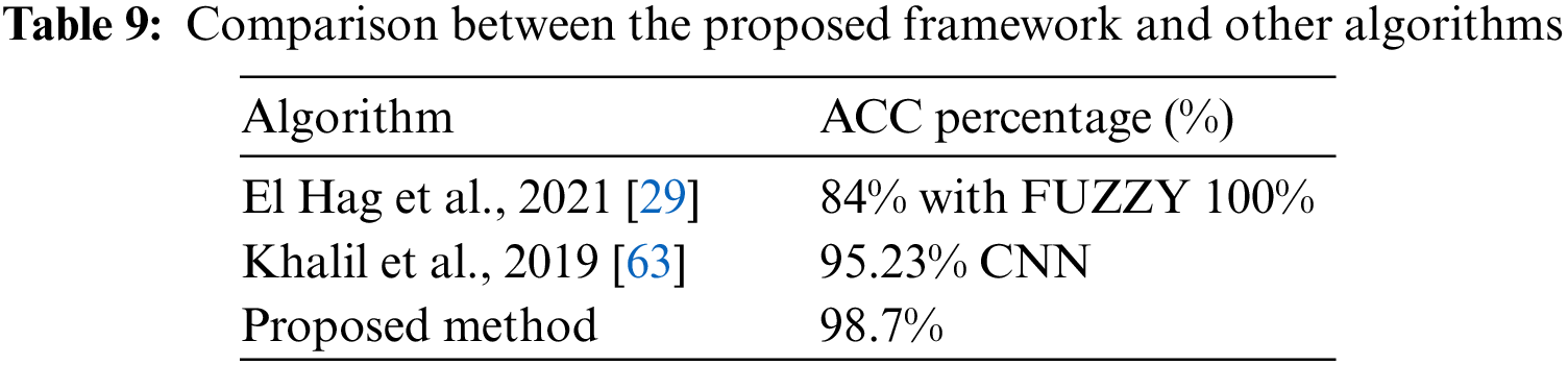
By comparing the obtained results from the proposed framework with other research [29,61], It can be concluded that the proposed model in this paper has achieved better ACC than the others. This is presented in Table 9.

5  Conclusion

This study evaluated the performance of four distinct datasets related to eye conditions: GL, CT, DR, and NDR. This article started by performing data cleansing to ensure the quality of the datasets. Afterward, they prepared the classes for initializing algorithms based on the VGG16CNN architecture. In this work, various parameters were adjusted and experimented with. The datasets were divided into training, validation, and testing sets using different ratios, such as 90% for training, 5% for validation, and 5% for testing, or 80% for training, 10% for validation, and 10% for testing. Dropout values, which help prevent overfitting, were set to 0.02 and 0.2. Multiple architectures were implemented and tested, leading to variations in the experimental setup.

The dropout was applied both with and without the CNN architecture or VGG16. To train and test the network for classifying the enhanced classes, a DTL approach was employed in this study. We used TL techniques to leverage pre-trained models and improve classification performance. The proposed model showed promising results when using AE-enhanced classes in combination with TL and CNN models. The achieved metrics included an ACC of 98.62%, an SPE of 98.65%, and a REC of 98.59%. The authors suggest several improvements further to enhance the model’s ACC for future work. One recommendation is to expand the dataset by adding new distinctive classes related to eye conditions. Increasing the diversity and size of the dataset can help the model generalize better and improve its performance. Additionally, incorporating new TL techniques beyond the ones used in this study may enhance the model’s capabilities and overall performance.

Acknowledgement: The authors thank the Department of Electrical Engineering, Faculty of Engineering, Benha University, for providing intellectual assistance.

Funding Statement: The authors received no specific funding for this study.

Author Contributions: The authors confirm their contribution to the paper as follows: study conception and design: Heba F. Elsepae and Heba M. El-Hoseny; data collection: Ayman S. Selmy and Heba F. Elsepae; analysis and interpretation of results: Heba F. Elsepae, Heba M. El-Hoseny and Wael A. Mohamed; draft manuscript preparation: Ayman S. Selmy and Wael A. Mohamed. All authors reviewed the results and approved the final version of the manuscript.

Availability of Data and Materials: The datasets generated during and/or analyzed during the current study are available from the corresponding author upon reasonable request.

Conflicts of Interest: The authors declare that they have no conflicts of interest to report regarding the present study.

References

1. L. Zhang, L. Tang, M. Xia and G. Cao, “The application of artificial intelligence in glaucoma diagnosis and prediction,” Frontiers in Cell and Developmental Biology, vol. 11, pp. 1–13, 2023. [Google Scholar]

2. E. Guallar, P. Gajwani, B. Swenor, J. Crews, J. Saaddine et al., “Optimizing glaucoma screening in high-risk population: Design and 1-year findings of the screening to prevent (stop) glaucoma study,” American Journal of Ophthalmology, vol. 180, pp. 18–28, 2017. [Google Scholar] [PubMed]

3. X. Q. Zhang, J. S. Fang, Y. Hu, R. Higashita, J. Liu et al., “Machine learning for cataract classification grading on ophthalmic imaging modalities: A survey,” Machine Intelligence Research, vol. 19, no. 3, pp. 184–208, 2022. https://doi.org/10.1007/s11633-022-1329-0 [Google Scholar] [CrossRef]

4. S. R. Flaxman, S. Resnikoff, R. R. Bourne, S. Resnikoff, P. Ackland et al., “Global causes of blindness and distance vision impairment 1990–2020: A systematic review and meta-analysis,” The Lancet Global Health, vol. 5, no. 12, pp. 1221–1234, 2017. [Google Scholar]

5. Y. Kumar and S. Gupta, “Deep transfer learning approaches to predict glaucoma, cataract, choroidal neovascularization, diabetic macular edema, drusen, and healthy eyes: An experimental review,” Archives of Computational Methods in Engineering, vol. 30, no. 1, pp. 521–541, 2023. [Google Scholar]

6. A. Kelkar, J. Kelkar, H. Mehta and W. Amoaku, “Cataract surgery in diabetes mellitus: A systematic review,” Indian Journal of Ophthalmology, vol. 66, no. 10, pp. 1401–1410, 2018. https://doi.org/10.1155/2021/6641944 [Google Scholar] [CrossRef]

7. N. Shaukat, J. Amin, M. Sharif, S. Kadry, L. Sevcik et al., “Classification and segmentation of diabetic retinopathy: A systemic review,” Applied Sciences, vol. 13, no. 5, pp. 1–25, 2023. [Google Scholar]

8. N. Shaukat, J. Amin, M. Sharif, F. Azam, S. Kadry et al., “Three-dimensional semantic segmentation of diabetic retinopathy lesions and grading using transfer learning,” Journal of Personalized Medicine, vol. 12, no. 9, pp. 1–17, 2022. https://doi.org/10.3390/jpm12091454 [Google Scholar] [PubMed] [CrossRef]

9. M. S. Junayed, M. B. Islam, A. Sadeghzadeh and S. Rahman, “CataractNet: An automated cataract detection system using deep learning for fundus images,” IEEE Access, vol. 9, pp. 128799–128808, 2021. https://doi.org/10.1109/ACCESS.2021.3112938 [Google Scholar] [CrossRef]

10. S. Duan, P. Huang, M. Chen, T. Wang, X. Sun et al., “Semi-supervised classification of fundus images combined with CNN and GCN,” Journal of Applied Clinical Medical Physics, vol. 23, no. 12, pp. 1–13, 2022. [Google Scholar]

11. V. Gulshan, L. Peng, M. Coram, M. Stumpe, A. Narayanaswamy et al., “Development and validation of a deep learning algorithm for detection of diabetic retinopathy in retinal fundus photographs,” JAMA, vol. 316, no. 22, pp. 2402–2410, 2016. https://doi.org/10.1001/jama.2016.17216 [Google Scholar] [PubMed] [CrossRef]

12. R. Kashyap, R. R. Nair, S. M. Gangadharan, S. Farooq, A. Rizwan et al., “Glaucoma detection and classification using improved U-Net deep learning model,” Healthcare, vol. 10, no. 12, pp. 1–19, 2022. [Google Scholar]

13. X. Li, T. Pang, B. Xiong, W. Liu, P. Liang et al., “Convolutional neural networks based transfer learning for diabetic retinopathy fundus image classification,” in 10th Int. Congress on Image and Signal Processing, Biomedical Engineering and Informatics (CISP-BMEI), Shanghai, China, pp. 1–11, 2017. [Google Scholar]

14. A. Krizhevsky, I. Sutskever and G. E. Hinton, “ImageNet classification with deep convolutional neural networks,” Communications of the ACM, vol. 60, no. 6, pp. 84–90, 2017. https://doi.org/10.1145/3065386 [Google Scholar] [CrossRef]

15. C. Szegedy, W. Liu, Y. Jia, P. Sermanet, S. Reed et al., “Going deeper with convolutions,” in Proc. of the IEEE Conf. on Computer Vision and Pattern Recognition, Boston, MA, USA, pp. 1–9, 2015. [Google Scholar]

16. K. Simonyan and A. Zisserman, “Very deep convolutional networks for large-scale image recognition,” in 3rd Int. Conf. on Learning Representations (ICLR 2015Computational and Biological Learning Society, San Diego, CA, USA, pp. 1–14, 2015. [Google Scholar]

17. W. Lu, Y. Tong, Y. Xing, C. Chen, Y. Shen et al., “Deep learning-based automated classification of multi-categorical abnormalities from optical coherence tomography images,” Translational Vision Science & Technology, vol. 7, no. 6, pp. 41, 2018. https://doi.org/10.1167/tvst.7.6.41 [Google Scholar] [PubMed] [CrossRef]

18. K. He, X. Zhang, S. Ren and J. Sun, “Deep residual learning for image recognition,” in Proc. of the IEEE Conf. on Computer Vision and Pattern Recognition, Las Vegas, NV, USA, pp. 770–778, 2016. [Google Scholar]

19. M. M. Kamal, M. H. Shanto, A. Hasnat, S. Sultana, M. Biswas et al., “A comprehensive review on the diabetic retinopathy, glaucoma and strabismus detection techniques based on machine learning and deep learning,” European Journal of Medical and Health Sciences, vol. 4, no. 2, pp. 24–40, 2022. [Google Scholar]

20. J. M. Ahn, S. Kim, K. S. Ahn, S. H. Cho, K. B. Lee et al., “A deep learning model for detecting both advanced and early glaucoma using fundus photography,” PLoS One, vol. 13, no. 11, pp. 1–8, 2018. [Google Scholar]

21. N. B. Thota and D. U. Reddy, “Improving the accuracy of diabetic retinopathy severity classification with transfer learning,” in 2020 IEEE 63rd Int. Midwest Symp. on Circuits and Systems (MWSCAS), Springfield, MA, USA, pp. 1003–1006, 2020. https://doi.org/10.1109/MWSCAS48704.2020.9184473 [Google Scholar] [CrossRef]

22. A. Sebastian, O. Elharrouss, S. Al-Maadeed and N. A. Almaadeed, “A survey on deep-learning-based diabetic retinopathy classification,” Diagnostics, vol. 13, no. 3, pp. 1–22, 2023. [Google Scholar]

23. C. Xu, X. Xi, X. Yang, L. Sun, L. Meng et al., “Local detail enhancement network for CNV typing in OCT images,” in 2022 15th Int. Conf. on Human System Interaction (HSI), Melbourne, Australia, pp. 1–5, 2022. https://doi.org/10.1109/HSI55341.2022.9869483 [Google Scholar] [CrossRef]

24. O. Khaled, M. El-Sahhar, Y. Talaat, Y. M. Hassan, A. Hamdy et al., “Cascaded architecture for classifying the preliminary stages of diabetic retinopathy,” in Proc. of the 9th Int. Conf. on Software and Information Engineering, Cairo, Egypt, pp. 108–112, 2020. [Google Scholar]

25. H. Pratt, F. Coenen, D. M. Broadbent, S. P. Harding and Y. Zheng, “Convolutional neural networks for diabetic retinopathy,” Procedia Computer Science, vol. 90, pp. 200–205, 2014. [Google Scholar]

26. M. T. Islam, S. A. Imran, A. Arefeen, M. Hasan and C. Shahnaz, “Source and camera independent ophthalmic disease recognition from fundus image using neural network,” in 2019 IEEE Int. Conf. on Signal Processing, Information, Communication & Systems (SPICSCON), Dhaka, Bangladesh, pp. 59–63, 2019. https://doi.org/10.1109/SPICSCON48833.2019.9065162 [Google Scholar] [CrossRef]

27. R. Sarki, K. Ahmed, H. Wang and Y. Zhang, “Automated detection of mild and multi-class diabetic eye diseases using deep learning,” Health Information Science and Systems, vol. 8, no. 1, pp. 1–9, 2020. [Google Scholar]

28. U. Raghavendra, H. Fujita, S. V. Bhandary, A. Gudigar, J. H. Tan et al., “Deep convolution neural network for accurate diagnosis of glaucoma using digital fundus images,” Information Sciences, vol. 441, pp. 41–49, 2018. https://doi.org/10.1016/j.ins.2018.01.051 [Google Scholar] [CrossRef]

29. N. A. El-Hag, A. Sedik, W. El-Shafai, H. M. El-Hoseny, A. A. Khalaf et al., “Classification of retinal images based on convolutional neural network,” Microscopy Research and Technique, vol. 84, no. 3, pp. 394–414, 2021. https://doi.org/10.1002/jemt.23596 [Google Scholar] [PubMed] [CrossRef]

30. A. Bali and V. Mansotra, “Transfer learning-based one versus rest classifier for multiclass multi-label ophthalmological disease prediction,” International Journal of Advanced Computer Science and Applications, vol. 12, no. 12, pp. 537–546, 2021. [Google Scholar]

31. M. K. Hasan, T. Tanha, M. R. Amin, O. Faruk, M. M. Khan et al., “Cataract disease detection by using transfer learning-based intelligent methods,” Computational and Mathematical Methods in Medicine, vol. 2021, pp. 1–11, 2021. https://doi.org/10.1155/2021/7666365 [Google Scholar] [PubMed] [CrossRef]

32. M. Z. Atwany, A. H. Sahyoun and M. Yaqub, “Deep learning techniques for diabetic retinopathy: A classification survey,” IEEE Access, vol. 10, pp. 28642–28655, 2022. https://doi.org/10.1109/ACCESS.2022.3157632 [Google Scholar] [CrossRef]

33. F. Li, Z. Liu, H. Chen, M. Jiang, X. Zhang et al., “Automatic detection of diabetic retinopathy in retinal fundus photographs based on deep learning algorithm,” Translational Vision Science & Technology, vol. 8, no. 6, pp. 4, 2019. https://doi.org/10.1167/tvst.8.6.4 [Google Scholar] [PubMed] [CrossRef]

34. I. Arias-Serrano, P. A. Velásquez-López, L. N. Avila-Briones, F. C. Laurido-Mora, F. Villalba-Meneses et al., “Artificial intelligence based glaucoma and diabetic retinopathy detection using MATLAB retrained AlexNet convolutional neural network,” F1000Research, vol. 12, no. 14, pp. 1–15, 2023. https://doi.org/10.12688/f1000research.122288.1 [Google Scholar] [CrossRef]

35. S. A. Kamran, K. F. Hossain, A. Tavakkoli, S. L. Zuckerbrod and S. A. Baker, “VTGAN: Semi-supervised retinal image synthesis and disease prediction using vision transformers,” in Proc. of the IEEE/CVF Int. Conf. on Computer Vision, Montreal, Canada, pp. 3235–3245, 2021. [Google Scholar]

36. T. J. Jebaseeli, C. A. Deva Durai and J. D. Peter, “Retinal blood vessel segmentation from depigmented diabetic retinopathy images,” IETE Journal of Research, vol. 67, no. 2, pp. 263–280, 2021. [Google Scholar]

37. M. Widyaningsih, T. K. Priyambodo, M. Kamal and M. E. Wibowo, “Optimization contrast enhancement and noise reduction for semantic segmentation of oil palm aerial imagery,” International Journal of Intelligent Engineering & Systems, vol. 16, no. 1, pp. 597–609, 2023. [Google Scholar]

38. J. Dissopa, S. Kansomkeat and S. Intajag, “Enhance contrast and balance color of retinal image,” Symmetry, vol. 13, no. 11, pp. 1–15, 2021. https://doi.org/10.3390/sym13112089 [Google Scholar] [CrossRef]

39. A. W. Salehi, S. Khan, G. Gupta, B. I. Alabduallah, A. Almjally et al., “A study of CNN and transfer learning in medical imaging: Advantages, challenges, future scope,” Sustainability, vol. 15, no. 7, pp. 1–28, 2023. [Google Scholar]

40. V. K. Velpula and L. D. Sharma, “Multi-stage glaucoma classification using pre-trained convolutional neural networks and voting-based classifier fusion,” Frontiers in Physiology, vol. 14, pp. 1–17, 2023. [Google Scholar]

41. C. Iorga and V. E. Neagoe, “A deep CNN approach with transfer learning for image recognition,” in 2019 11th Int. Conf. on Electronics, Computers and Artificial Intelligence (ECAI), Pitesti, Romania, pp. 1–6, 2019. [Google Scholar]

42. P. Mathur, T. Sharma and K. Veer, “Analysis of CNN and feed-forward ANN model for the evaluation of ECG signal,” Current Signal Transduction Therapy, vol. 18, no. 1, pp. 1–8, 2023. [Google Scholar]

43. M. Vakalopoulou, S. Christodoulidis, N. Burgos, O. Colliot and V. Lepetit, “Deep learning: Basics and convolutional neural networks (CNNs),” in Machine Learning for Brain Disorders, 1stedition, Saskatoon, Canada: Humana Press, pp. 77–115, 2023. https://doi.org/10.1007/978-1-0716-3195-9 [Google Scholar] [CrossRef]

44. M. M. Taye, “Theoretical understanding of convolutional neural network: Concepts, architectures, applications, future directions,” Computation, vol. 11, no. 3, pp. 1–23, 2023. https://doi.org/10.3390/computation11030052 [Google Scholar] [CrossRef]

45. Y. Gong, L. Wang, R. Guo and S. Lazebnik, “Multi-scale orderless pooling of deep convolutional activation features,” in European Conf. on Computer Vision, Zurich, Switzerland, pp. 392–407, 2014. [Google Scholar]

46. T. Szandała, “Review and comparison of commonly used activation functions for deep neural networks,” in Bio-Inspired Neurocomputing, 1stedition, Warszawa, Poland: Springer Singapore, pp. 203–225, 2020. https://doi.org/10.1007/978-981-15-5495-7_1 [Google Scholar] [CrossRef]

47. A. A. Mohammed and V. Umaashankar, “Effectiveness of hierarchical softmax in large scale classification tasks,” in 2018 Int. Conf. on Advances in Computing, Communications, and Informatics (ICACCI), Bangalore, India, pp. 1090–1094, 2018. https://doi.org/10.1109/ICACCI.2018.8554637 [Google Scholar] [CrossRef]

48. Y. Zheng, B. Danaher and M. Brown, “Evaluating the variable stride algorithm in the identification of diabetic retinopathy,” Beyond Undergraduate Research Journal, vol. 6, no. 1, pp. 1–9, 2022. [Google Scholar]

49. S. S. Basha, S. R. Dubey, V. Pulabaigari and S. Mukherjee, “Impact of fully connected layers on performance of convolutional neural networks for image classification,” Neurocomputing, vol. 378, pp. 112–119, 2020. https://doi.org/10.1016/j.neucom.2019.10.008 [Google Scholar] [CrossRef]

50. M. Iman, H. R. Arabnia and K. Rasheed, “A review of deep transfer learning and recent advancements,” Technologies, vol. 11, no. 2, pp. 1–14, 2023. https://doi.org/10.3390/technologies11020040 [Google Scholar] [CrossRef]

51. G. V. Doddi, “Preprocessed_eye_diseases_fundus_images,” [Online]. Available: https://www.kaggle.com/datasets/gunavenkatdoddi/preprocessed-eye-diseases-fundus-images (accessed on 02/09/2023). [Google Scholar]

52. M. Aatila, M. Lachgar, H. Hrimech and A. Kartit, “Diabetic retinopathy classification using ResNet50 and VGG-16 pretrained networks,” International Journal of Computer Engineering and Data Science (IJCEDS), vol. 1, no. 1, pp. 1–7, 2021. [Google Scholar]

53. T. Aziz, C. Charoenlarpnopparut and S. Mahapakulchai, “Deep learning-based hemorrhage detection for diabetic retinopathy screening,” Scientific Reports, vol. 13, no. 1, pp. 1–12, 2023. [Google Scholar]

54. C. Bhardwaj, S. Jain and M. Sood, “Diabetic retinopathy severity grading employing quadrant-based Inception-V3 convolution neural network architecture,” International Journal of Imaging Systems and Technology, vol. 31, no. 2, pp. 592–608, 2021. https://doi.org/10.1002/ima.22510 [Google Scholar] [CrossRef]

55. T. Araújo, G. Aresta, L. Mendonça, S. Penas, C. Maia et al., “Data augmentation for improving proliferative diabetic retinopathy detection in eye fundus images,” IEEE Access, vol. 8, pp. 182462–182474, 2020. [Google Scholar]

56. M. Xiao, Y. Wu, G. Zuo, S. Fan, Z. A. Shaikh et al., “Addressing overfitting problem in deep learning-based solutions for next generation data-driven networks,” Wireless Communications and Mobile Computing, vol. 2021, pp. 1–10, 2021. https://doi.org/10.1155/2021/8493795 [Google Scholar] [CrossRef]

57. N. Srivastava, G. Hinton, A. Krizhevsky, I. Sutskever and R. Salakhutdinov, “Dropout: A simple way to prevent neural networks from overfitting,” The Journal of Machine Learning Research, vol. 15, no. 1, pp. 1929–1958, 2014. [Google Scholar]

58. A. Defazio and S. Jelassi, “Adaptivity without compromise: A momentumized, adaptive, dual averaged gradient method for stochastic optimization,” The Journal of Machine Learning Research, vol. 23, no. 1, pp. 6429–6462, 2022. [Google Scholar]

59. R. H. Paradisa, A. Bustamam, A. A. Victor, A. R. Yudantha and D. Sarwinda, “Diabetic retinopathy detection using deep convolutional neural network with visualization of guided grad-CA,” in 4th Int. Conf. of Computer and Informatics Engineering (IC2IE), Depok, Indonesia, pp. 19–24, 2021. https://doi.org/10.1109/IC2IE53219.2021.9649326 [Google Scholar] [CrossRef]

60. E. M. El Houby, “Using transfer learning for diabetic retinopathy stage classification,” Applied Computing and Informatics, vol. 1, no. 1, pp. 1–11, 2021. https://doi.org/10.1108/ACI-07-2021-0191 [Google Scholar] [CrossRef]

61. F. S. Nahm, “Receiver operating characteristic curve: Overview and practical use for clinicians,” Korean Journal of Anesthesiology, vol. 75, no. 1, pp. 25–36, 2022. https://doi.org/10.4097/kja.21209 [Google Scholar] [PubMed] [CrossRef]

62. A. A. Ahmed, E. H. Salama, H. A. Shehata and A. K. Noreldin, “The role of Ischemia modified albumin in detecting diabetic nephropathy,” SVU-International Journal of Medical Sciences, vol. 6, no. 1, pp. 359–367, 2023. https://doi.org/10.21608/svuijm.2022.165289.1419 [Google Scholar] [CrossRef]

63. H. Khalil, N. El-Hag, A. Sedik, W. El-Shafie, A. E. Mohamed et al., “Classification of diabetic retinopathy types based on convolution neural network (CNN),” Menoufia Journal of Electronic Engineering Research, vol. 28, pp. 126–153, 2019. [Google Scholar]