
 Submit a Paper
 Propose a Special lssue
 Open Access
ARTICLE

Learning Dual-Domain Calibration and Distance-Driven Correlation Filter: A Probabilistic Perspective for UAV Tracking
1 Jiangsu Province Key Lab on Image Processing and Image Communication, Nanjing University of Posts and Telecommunications, Nanjing, China
2 School of Computer Science, Qufu Normal University, Qufu, China
3 National Engineering Research Center of Communication and Network Technology, Nanjing University of Posts and Telecommunications, Nanjing, China
* Corresponding Author: Lizhen Deng. Email:
(This article belongs to the Special Issue: AI Powered Human-centric Computing with Cloud and Edge)
Computers, Materials & Continua 2023, 77(3), 3741-3764. https://doi.org/10.32604/cmc.2023.039828
Received 19 February 2023; Accepted 01 July 2023; Issue published 26 December 2023
 View Full Text
 Download PDF
Abstract
Unmanned Aerial Vehicle (UAV) tracking has been possible because of the growth of intelligent information technology in smart cities, making it simple to gather data at any time by dynamically monitoring events, people, the environment, and other aspects in the city. The traditional filter creates a model to address the boundary effect and time filter degradation issues in UAV tracking operations. But these methods ignore the loss of data integrity terms since they are overly dependent on numerous explicit previous regularization terms. In light of the aforementioned issues, this work suggests a dual-domain Jensen-Shannon divergence correlation filter (DJSCF) model address the probability-based distance measuring issue in the event of filter degradation. The two-domain weighting matrix and JS divergence constraint are combined to lessen the impact of sample imbalance and distortion. Two new tracking models that are based on the perspectives of the actual probability filter distribution and observation probability filter distribution are proposed to translate the statistical distance in the online tracking model into response fitting. The model is roughly transformed into a linear equality constraint issue in the iterative solution, which is then solved by the alternate direction multiplier method (ADMM). The usefulness and superiority of the suggested strategy have been shown by a vast number of experimental findings.Keywords
Smart cities [1] are increasingly emerging as the primary outcome of urbanization and information technology integration as social intelligence advances. Six-generation (6G) technology [2] supports intelligent interconnection of human-machine objects and can generate potential application scenarios [3] such as full regional coverage by making full use of full spectrum resources. However, smart cities lack the support of spatial geographic information, and the application scenarios usually require terminal devices to provide more processing power and are more sensitive to transmission delays. However, current devices typically have poor processing power, and the centralized architecture of traditional cloud computing networks may result in poor transmission latency [4]. With the development of the Internet of Things (IoT) [5–10], information data is extracted in a timely manner using big data technologies, and edge computing servers are deployed at the edge of the network through mobile edge computing (MEC) [11–13]. This can effectively solve the problems of sensitive transmission delay and insufficient computing power of mobile terminals [14], and facilitate the provision of sufficient information for smart city construction [15–18]. In MEC networks, UAVs are highly flexible and operable and can dock space networks with ground networks to collaboratively build three-dimensional networks [19]. UAVs are able to dynamically adjust their deployment position in the network by tracking and adaptively responding to changes in the network environment [20]. UAVs’ visual tracking has been used for aerial refueling [21], aerial aircraft tracking [22], and target tracking [23,24]. Although there have been many successful research results in visual tracking, it still remains a difficult point to achieve high robustness and accuracy visual tracking with the influence of environmental factors such as occlusion, target in-plane/out-plane rotation, fast motion, blurring, lighting, and deformation, etc.
Recently, discriminative correlation filters (DCFs) [25] based tracking methods have received widespread attention [26–28]. However, these methods have caused the boundary effect problem with adverse effects on tracking performance while using the circular matrix which is calculated in the frequency domain to improve the model efficiency. Therefore, if it is affected by aberrance in challenging scenes. Compared with ordinary target tracking, the targets in the UAV domain are often very small and the existing DCF methods are definitely sensitive to handle the small targets in this case [29,30]. The existing DCF methods estimate the center position of the target, and the tracking model will continue to degenerate in the sequences [28]. Thus, if the target is small and similar to the background, UAV tracking is more prone to template drift and model degradation during the learning process.
A variety of visual tracking methods based on DCF have been proposed, and most of the successful strategies are applied to solve the above model degradation problem. For example, spatially regularized discriminative correlation filters (SRDCF) [31] and spatial-temporal regularized correlation filters (STRCF) [32] used spatial regularization and space-time regularization to solve boundary effects. In addition, STRCF mitigates the degradation of time filtering by introducing penalty terms in the context of SRDCF, which makes the tracker subject to more noise interference and reduces tracking reliability. And adaptive spatially-regularized correlation filters (ASRCF) [33] used the adaptive spatial regularization method to further improve the estimation ability of object perception and obtain more reliable filter coefficients. Many DCFs based trackers have suppressed the boundary effects by expanding the search area to obtain better tracking effects. The background-aware correlation filter (BACF) [34] used a cropping matrix to extract patches densely from the background and expand the search area at a lower computational cost. Group feature selection method for discriminative correlation filters (GFS-DCF) [35] advocates channel selection in DCF-based tracking and used an effective low-rank approximation [36]. The filter constraint here can smoothly realize the temporal information and adaptively integrate historical information to achieve group feature selection across channels and spatial dimensions. In order to get accurate tracking, a large margin object tracking method with circulant feature maps (LMCF) [37] and an attentional correlation filter network (ACFN) [38], tried to suppress the possible abnormalities through some measures. To solve the aberrance problem of response maps, the aberrance repressed correlation filter (ARCF) [39] added a regular term on the basis of BACF which can suppress the mutation of the response maps and used Euclidean distance to define the direct response approximation between the two response maps. In addition, in order to deal with the problem of boundary discontinuity and sample contamination caused by the cosine window, Li et al. [40] proposed a spatial regularization method to remove the cosine window and further introduced binary and Gaussian shape mask functions to eliminate the boundary problem.
For UAV tracking, there are also some special strategies in the DCF framework. Semantic-aware real-time correlation tracking framework (SARCT) [41] introduced a semantic-aware DCF-based framework for UAV tracking by combing the semantic segmentation module and sharing features for the object detection module and semantic segmentation. Also, the part-based mechanism was also combined with BACF in [42] and the Bayesian inference approach was proposed to achieve a coarse-to-fine strategy. AutoTrack [43] proposed a new method for online automatic adaptive learning of spatiotemporal regularization terms, which uses spatial local response map variants as spatial regularization, so that DCF focuses on the learning of the trusted part of the object, and determines the update processing of the filter according to the global response map variants. Overall, these existing methods share some commonalities. In particular, they often heavily rely on a presumed fixed spatial or temporal filter learning and fixed response map approximation.
In this paper, UAV tracking is sufficiently far away from the object in traditional tracking scenarios that the small target is fundamentally limited by less knowledge used in online learning and a more unbalanced sample problem. While many existing works focus on the sparsity [44] in spatial smooth or temporal smooth, the direct coupling of the several regularization terms used in several works like [34,41–43] is not a good choice, and the online filter learning will be obfuscated by redundancy. Therefore, it is interesting to ask the problem concerned in this work: what can we measure in online learning: probabilistic response fitting or direct response approximation?
From the perspective of actual and observed probability filter distribution in small targets for UAV tracking, the probabilistic response fitting in temporal smooth is more robust than the direct response approximation. Although Euclidean distance is useful, it is limited by the largest-scaled feature that would dominate the others. It is hard to judge the “best” similarity measure or a best-performing measure here. In general, we are the first work to transfer the statistical distance to correlation response fitting in the online tracking model. It also could shed light on the performance and behavior of measures in deep learning works like [45]. Although the insights of this work are the most similar to our work, the main truth is that the distribution assumption is different.
Furthermore, a novel unsupervised method called maximally divergent intervals (MDI) [46] searched for continuous intervals of time and region in a space containing anomalous events instead of analyzing the data point by point and attempted to use KL divergence and unbiased KL divergence to achieve better detection results. Not only that, but MDI also introduced JS divergence to demonstrate the superiority of the model and improve its scalability of the model. Similarly, Jiang et al. in [47] also used KL divergence to search for abnormal blocks in higher-order tensors. At the beginning of signal processing, the KL and JS divergence was used to fit the matching degree of the two distribution signals. Inspired by this, we consider the similarity search between the response maps of the filters as the curve fitting problem between the adjacent frame filters. It should be noted that the original Euclidean distance is not applicable because it is prone to filter under-fitting learning. Actually, the under-fitting problem had recently been mentioned in feature embedding problems like [48]. While it seems to be rather complicated to estimate a probabilistic response fitting by the above KL or JS procedure, the main benefit of estimating the mean and the covariance lies in the inherent regulation properties in our correlation filter response term.
While the KL divergence and JS divergence can achieve a good fitting effect. In addition, since the fitting object in the KL divergence is the response map of the adjacent frame filter to the image block [39], the KL divergence term can ensure that the filter has the highest similarity in the response map in the time domain. Therefore, our model uses a temporal-response calibrated filter based on the KL divergence. Since the KL divergence does not measure the distance between the two distributions in space, the KL divergence can be considered as a measure of the information loss of the response maps in the filter in our algorithm. Then we can find the target with the highest response value in the time domain according to the principle of function loss minimization, which is considered our tracking target. Experiments have shown that trackers based on temporal-response calibrated filters have greatly improved accuracy.
Based on the above-mentioned analysis, we propose a new model named AKLCF. Specifically, we use KL divergence fitting to mitigate the under-fitting of the Euclidean distance. In addition, to ensure the validity of the model, we add model confidence terms to avoid the variations of the model that occurred during the optimization process, which greatly improves the stability of the model. The algorithm flow chart of AKLCF is shown in Fig. 1a. Specifically, the multi-channel features are extracted from the previous frame of an image. We use KL divergence to calculate the similarity between response maps, and then build the learning model of AKLCF. At the same time, we further use the JS divergence to investigate the impact of the similarity measurement method on the tracking effect of related filters and propose the AJSCF model. The algorithm flow chart of AJSCF is shown in Fig. 1b. Notice that AJSCF is different from AKLCF in divergence. Compared with KL divergence, JS divergence solves the problem of asymmetry of KL divergence and avoids the “gradient disappearance” problem in the process of KL divergence fitting, thereby improving the tracking effect of the model.
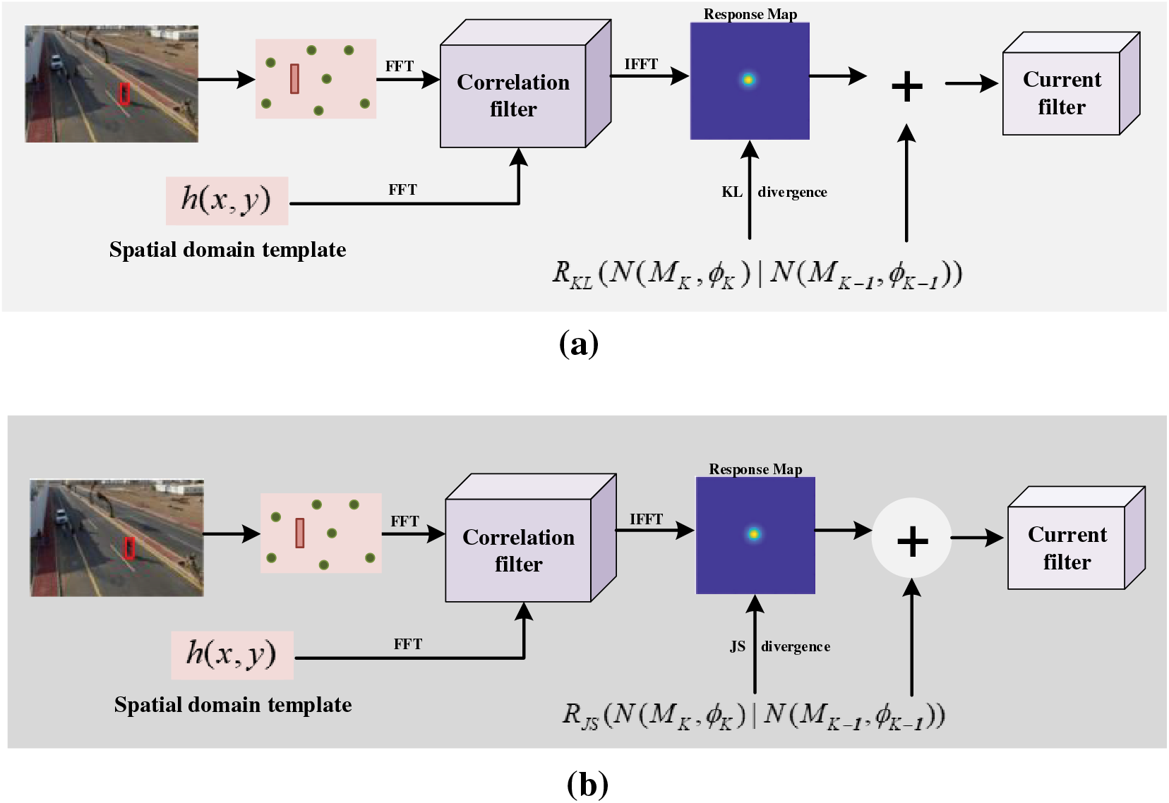
Figure 1: The algorithm flowcharts of aberrance Kullback-Leibler (KL) divergence correlation filter (AKLCF) and aberrance Jensen-Shannon (JS) divergence correlation filter (AJSCF). The structure of the two flowcharts is the same and the main difference is that the former uses KL divergence to achieve similarity fitting, while the latter uses JS divergence
The UAV tracking will be further influenced by the imbalance of positive and negative samples during training DCF. Although kernelized correlation filter (KCF) [49] gave continuous weighting to samples with different offsets by continuous labeling, and could effectively detect target samples of interest to a certain extent and improve the accuracy of visual tracking, it does not solve the adverse effects of imbalance of positive and negative samples on visual tracking. Therefore, inspired by the collaborative distribution alignment (CDA) model [50], we propose a dual-domain Jensen-Shannon divergence correlation filter (DJSCF) model, which introduces dual-domain weighting into the data items of the loss function, uses a weighting method to suppress the influence of the imbalance of positive and negative samples and combines JS divergence to improve the accuracy of target tracking. The algorithm flow chart of DJSCF is shown in Fig. 2. DJSCF adds the sorting and selection of features on the basis of AJSCF, which is realized by dual-domain weighting, and effectively alleviates the problem of imbalance between samples.
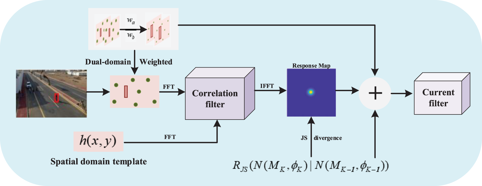
Figure 2: The flow chart of dual-domain Jensen-Shannon divergence correlation filter (DJSCF)
The main contributions of this work are shown as follows:
• To address the under-fitting of the response approximation in the Euclidean distance domain, we suggest the AKLCF model, which makes use of KL divergence fitting. The distortion brought on by noise can be efficiently reduced by the filter based on temporal response calibration. To further assure the model’s validity, we also include model confidence terms.
• We introduce JS divergence to propose the AJSCF model, which validates the impact of measurement methods on tracking accuracy and enhances the richness and verifiability of article content, in order to address the asymmetry of KL divergence and the disappearance of gradient.
• In order to address the issue of sample imbalance, we present a DJSCF model with JS divergence fitting that incorporates two-domain weighting due to two diagonally weighted matrices in the sparse data item. Several tests were carried out to demonstrate the excellence of our DJSCF.
Target tracking mainly uses the tracking algorithm to select the one with the highest similarity to the target object as the target of the next frame, and then obtains the motion trajectory of the target object in the entire video sequence. Therefore, how accurately represent the similarity between the candidate block and the target block is an important factor that determines the accuracy of target tracking. As the research of target tracking and the difficulty of tracking tasks continue to increase, the distance similarity measurement methods used by tracking algorithms are also continuously improved. In image processing and analysis theory, common similarity measurement methods include Euclidean distance, block distance, checkerboard distance, weighted distance, Bart Charlie coefficient, Harsdorf distance, etc. Among them, Euclidean distance is the most applied and simplest.
The most commonly used mathematical expression of the Euclidean distance is the norm, which is mainly divided into four norms. Among them, the target tracking algorithm often uses the
When the probability of an event is
From the KL divergence formula, we can see that the closer the distribution of Q is to P (the more fitting the Q distribution is to P), the smaller the divergence value is, that is, the smaller the loss value is. Because the logarithmic function is convex, the value of KL divergence is non-negative. KL divergence is sometimes called KL distance, but it does not satisfy the property of distance. Because KL divergence is not symmetric and KL divergence does not satisfy triangle inequality. In machine learning, KL divergence can be used to evaluate the gap between label and predictions. In the process of optimization, we only need to pay attention to the cross entropy.
In probability statistics, JS divergence has the same ability to measure the similarity of two probability distributions as KL divergence. Its calculation method is based on KL divergence and inherits the non-negative nature of KL divergence. However, there is one important difference: JS divergence has symmetry. The formula of JS divergence is as follows: set two probability distributions as P and Q,
If the two distributions P and Q are far apart and completely do not overlap, then the KL divergence value is meaningless, while the JS divergence value is a constant
Due to the differences in background, light, sensor resolution, and other aspects, the data collected by UAVs in different scenes may be in different data domains. There are different numbers of positive samples and negative samples in each domain, and the number of negative samples (background) is far greater than the number of positive samples (target) in single-target tracking. The problem of sample imbalance will lead to the over-fitting of a large sample proportion, and the prediction will tend to classify with more samples. Therefore, there is a strong need to align the number of samples between different domains and train the data to find samples suitable for the target domain. Inspired by the trilateral weighted sparse coding scheme (TWSC) in [51] and the dual-domain collaboration in [50], we use the method of two-field weighting to increase the weight of samples, that is, to add a larger weight to the samples with a smaller number of samples, and to add a smaller weight to the samples with a larger number of samples.
In the model, we introduce two diagonal matrices,
where x is the positive sample, y is the negative sample. Our method also introduces the idea of dual-domain weighting, and the supporting materials show the specific processing operations of
3 The Dual-Domain Collaboration and Distances Correlation Filters
In this section, we first introduce the AKLCF and explain the role of KL divergence in the model tracking process. We further make the derivation of the optimization process in detail. Then, we introduce and derive DJSCF in detail, and introduce how dual-domain weighting and JS divergence can jointly improve the accuracy and robustness of target tracking. Considering that our model is based on the similarity of response maps, Fig. 2 shows the response effect graphs of the three methods. The trackers learn both positive samples (red sample) of objects and negative samples (green sample) in the background.
3.1 Aberrance Kullback-Leibler Divergence Correlation Filter (AKLCF) Model
Our AKLCF optimizes the response approximation in Euclidean distance to the KL divergence to achieve the curve fitting of the filters. In addition, the AKLCF increases the model confidence to improve the reliability of the model. Below we detail the construction of model functions. For simplicity, let
Then, we replace the third term of Eq. (4) with the function
As discussed above, in the formula with Eq. (5) add of is replaced by the Kullback-Leibler divergence term. In addition, we add a model confidence term to ensure the reliability of the model. Then we improve the loss functions by minimizing the following unconstraint objective:
where
To better reflect the effect of the KL divergence term, we first analyze it in detail to obtain the specific expression of the KL divergence term. Since the KL divergence is a measure of the asymmetry of the difference between the two probability distributions. In our model, the KL divergence is used to measure the difference between the convolution matrix of the current frame and the previous frame, that is:
where
For convenience, we assume that the value vectors of filter and image blocks have multivariate Gaussian distributions, then the convolution matrix also has a Gaussian distribution, i.e.,
We substitute the specific expression of the model confidence term and Eq. (8) into Eq. (6) to get:
In general, the first term of the formula is data fidelity, the second is the space penalty, and the third and fourth terms are our improved contents, namely the model confidence term and the KL divergence term.
3.2 The Dual-Domain Jensen-Shannon Divergence Correlation Filter (DJSCF) Model
DJSCF adds dual-domain weighted matrices and JS divergence in the response map which need to be considered in the optimization process, therefore the construction of the loss function in DJSCF tracker is described in detail below:
Let
Similar to AKLCF, we use JS divergence and model confidence to improve the third term of the objective function, and get the objective function as follows:
It equals to:
Since the JS divergence is proposed based on the KL divergence, we use two covariance matrices (
The AJSCF model is a version that only replaces the KL divergence of AKLCF with JS divergence. The comparison between AJSCF and AKLCF shows the superiority of JS divergence in similarity fitting. At the same time, the latter DJSCF is obtained by adding dual-domain weighting based on AJSCF. And comparing AJSCF with DJSCF can verify the effect of dual-domain weighting on tracking performance.
3.3 ADMM Decomposition of AKLCF and DJSCF
AKLCF: The model in Eq. (9) is a convex problem and can be minimized with the ADMM algorithm to obtain the global optimal solution. Since Eq. (9) has a convolution calculation in the time domain, Pasival’s theorem is used to facilitate the calculation by converting the problem into the frequency domain. Then we get the objective function in the frequency domain as follows:
where the superscript
According to Eq. (8) and Pasival’s theorem, the KL divergence term in the frequency domain is expressed as follows:
Substitute Eq. (17) into Eq. (16), and using Pasival’s theorem, then we get the specific optimization function.
where
DJSCF: Similar to AKLCF, according to Pasival’s theorem, we get:
We get the optimization formulation:
According to the principle of JS divergence and Eq. (8), we get:
Then the optimization solution of DJSCF is implemented by ADMM and is divided into the following subproblems:
3.4 Solution of Sub-Problems of Two Models
From Eqs. (19) and (23), it is easy to find that except for the subproblem
Solution to subproblem
The solution to subproblem
where
Solution to subproblem:
In AKLCF model, the augmented Lagrangian form is expressed as follows:
Using the ADMM algorithm, two sub-problems can be obtained, namely:
Unfortunately, since subproblem
The subproblem
Each smaller problem can be efficiently calculated and the solution is presented below:
where
Finally, the solution of
According to the ADMM algorithm, the
Then the solution of
In the actual calculation process,
Similar to Eq. (28), the subproblem
After iterative calculation,
The solutions of the weighted matrices
where the parameter
The core idea of matrix update is to set non-diagonal elements to 0 and reorder the diagonal elements to assign values [52,53]. The specific method is to arrange the elements on the diagonal from small to large and replace the original value with the sort position number of each element. For example, if the
where
Update of Lagrangian Parameter:
The Lagrangian parameter is updated according to the following equation:
where the subscript i and
Updating of appearance model:
The appearance model updating takes an important influence on visual tracking. The appearance of tracked objects often changes in the tracking process under the effect of posture, scale, occlusion, and rotation. Therefore, we apply an online update strategy to update the appearance model and improve the robustness of our method. The appearance model at frame t can be updated as follows:
where
In each iterative calculation of subproblem f, the transformation of Fast Fourier Transform (FFT) and Inverse Fast Fourier Transform (IFFT) needs to be performed, then the computational complexity is
To demonstrate the superiority and effectiveness of our proposed models, we compare them with several state-of-the-art trackers with the HOG and deep features. We chose the 19-layer deep convolutional neural network VGG19 [54] (Visual Geometry Group) to extract the deep features in our experiments. In order to better explore the robust performance of the models, we conduct comparative experiments on different data sets. The value of
4.1 Experiment Datasets and Baseline Methods
We evaluated the performance of AKLCF, AJSCF, DJSCF, and other trackers on four benchmark datasets, including UAV123@10fps [55], DTB70 [29], UAVDT-S [30], UAVDT-M [30] and VisDrone2018-test-dev [56] datasets. UAV123 contains 123 video sequences, which is the most commonly used and most comprehensive data set for UAV tracking. DTB70 contains 70 video sequences. UAVDT-S and UAVDT-M are made up of 50 challenging videos respectively. It is worth noting that the UAVDT-M data set is used to detect the performance of multi-target tracking, and we modified it to make it also able to judge the performance of our single-target tracker. The VisDrone2018-test-dev dataset has 35 challenging videos. All evaluation criteria are according to the original protocol defined in three benchmarks, respectively [29,30,55]. We measured the performance of the tracking methods with one-pass evaluation (OPE) [57]. The evaluation method of OPE makes use of marking the real target frame in the first frame of the video sequence, no longer marks the target in the next frame number of images, and carries out a complete tracking of the entire video sequence. The common indicators of OPE are success plots and precision plots. The average pixel error averages the detection error of all frames. If the tracking fails due to accidental factors, it will have a certain impact on the result of this indicator, and the size of the impact is related to the number of frames of accidental factors. When the overlap rate of a frame is greater than the set threshold, take the horizontal axis as the threshold of the overlap threshold and the vertical axis as the success rate to obtain the success plots. The precesion plots are similar to the success plots. The horizontal axis is the threshold, and the vertical axis is the ratio of the number of frames below a certain threshold to the total number of frames. The threshold setting condition is the distance between the detection center and the real target center. When the distance is less than a certain threshold, it is considered to meet the precision. The results are compared with 15 state-of-the-art trackers with both HOG feature-based trackers (i.e., ARCF-HC [39], LADCF [52], STRCF [32], SRDCF [31], DSST [58], SAMF [59], KCF [49], GFSDCF [35], AutoTrack [43], ECO-HC (with gray-scale) [60], Histograms of Oriented Gradients (HOG-LR) [61]) and deep-based trackers (i.e., ECO [60], CCOT [62], ASRCF [33], MDNet [63], ADNet [64], CFNet [65], CREST [66], MCPF [67], SiamFC [68], and HDT [69]).
4.2 Quantitative Analysis of Tracking Dataset
First of all, we compared the overall performance of AKLCF, AJSCF, and DJSCF with other state-of-the-art hand-crafted trackers on UAV123@10fps [55], DTB70 [29], UAVDT-S [30], UAVDT-M [30] and VisDrone2018-test-dev [56] datasets. The comparison results are shown in Fig. 3. From the resulting graph, it can be seen that each comparison method performs best on the dataset UAVDT-M. Due to the limitations of feature extraction ability and computational process, traditional HOG-based methods perform slightly worse than correlation filters and deep learning-based methods. A class of methods based on discriminant correlation filters, combined with spatial adaptation or structured support vector machines, have good computational efficiency and positioning performance and perform well on various datasets. However, the method based on deep learning pays more attention to accuracy and therefore has greater computational complexity. On five different datasets, our method has an accuracy rate that exceeds the lower-performing method by nearly 25%. Even in this individual case on the UAVDT-M dataset, our method is only 0.1% less accurate than the first-place AutoTrack. Therefore, experimental results comparing multiple datasets show that our method has strong competitiveness in tracking target detection.
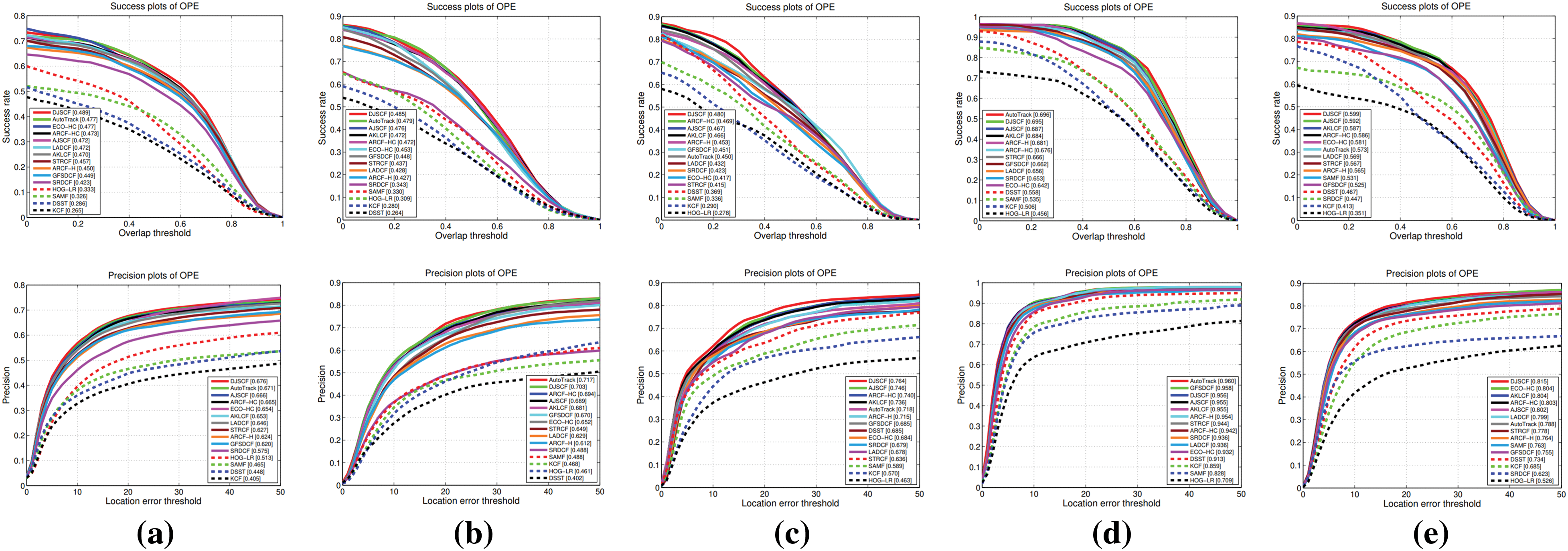
Figure 3: Precision and success plots of proposed methods as well as other HOG feature-based trackers on (a) UAV123@10fps (first column), (b) DTB70 (second column), (c) UAVDT-S (third column), (d) UAVDT-M (fourth column) and (e) VisDrone2018-test-dev (fifth column). Precision and AUC are marked in the precision plots and success plots, respectively
4.3 Quantitative Analysis of Variants and Deep Feature Configuration
We carried out comparative studies in several representative scenarios, such as background clutter, illumination changes, partial occlusion, size changes, and viewpoint shifts, to reflect the tracking performance of DJSCF in various contexts. Fig. 4 also displays the attribute-based performance of each tracker, with each group representing a distinct attribute. In general, a tracker that uses deep learning outperforms other trackers by a large margin. We discovered that all trackers had the lowest scores when it came to background clutter problems, additionally, some trackers struggle with scale change characteristics. Since particle filter frameworks can more effectively explore state space, we can find that particle filter-based approaches (i.e., HOG-LR) are superior to local sliding window-based methods (i.e., DSST and KCF) for qualities relevant to motion models.
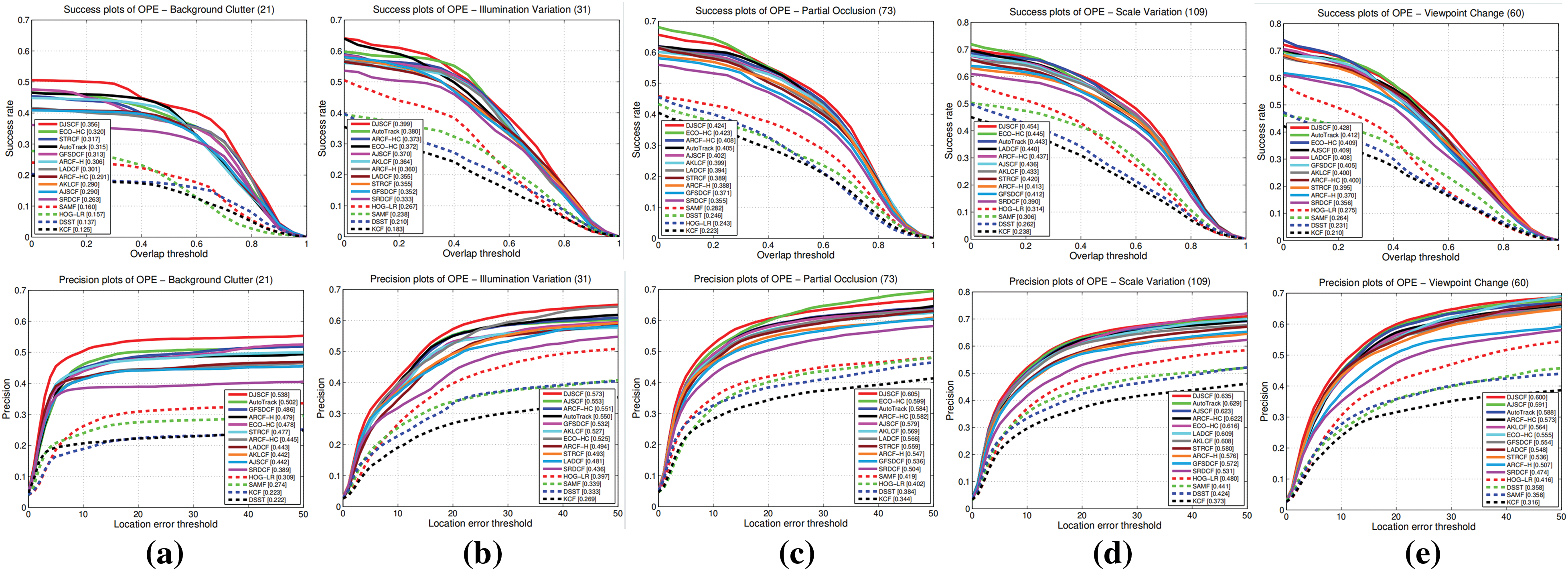
Figure 4: Attributes of proposed methods as well as other HOG feature-based trackers including (a) background clutter (first column), (b) illumination variation (second column), (c) partial occlusion (third column), (d) scale variation (fourth column), and (e) viewpoint change (fifth column). Precision and area under the curve (AUC) are marked in the precision plots and success plots, respectively
To further accurately assess the performance of our AKLCF, AJSCF, and DJSCF, we compared the trackers on the UAVDT-S dataset with deep features. DJSCF, AJSCF, and AKLCF took the top three positions on both the precision and success plots, as shown in Fig. 5. Due to the introduction of a weighting matrix to balance the number of positive and negative samples in DJSCF, the effect is better than AJSCF, with values greater than AJSCF by about 1.5%. In terms of precision plots, DJSCF, AJSCF, and AKLCF outperform ECO (0.702), which has good performance on numerous datasets, by 8.83%, 6.27%, and 4.84%, and MDNet (0.725), which was rated fourth. The DJSCF score is significantly greater than that of other trackers when it comes to success plots. In comparison to MDNet, which is in fourth position, DJSCF is 3.45% higher, while ECO, which is in fifth place, is 6.43% higher.
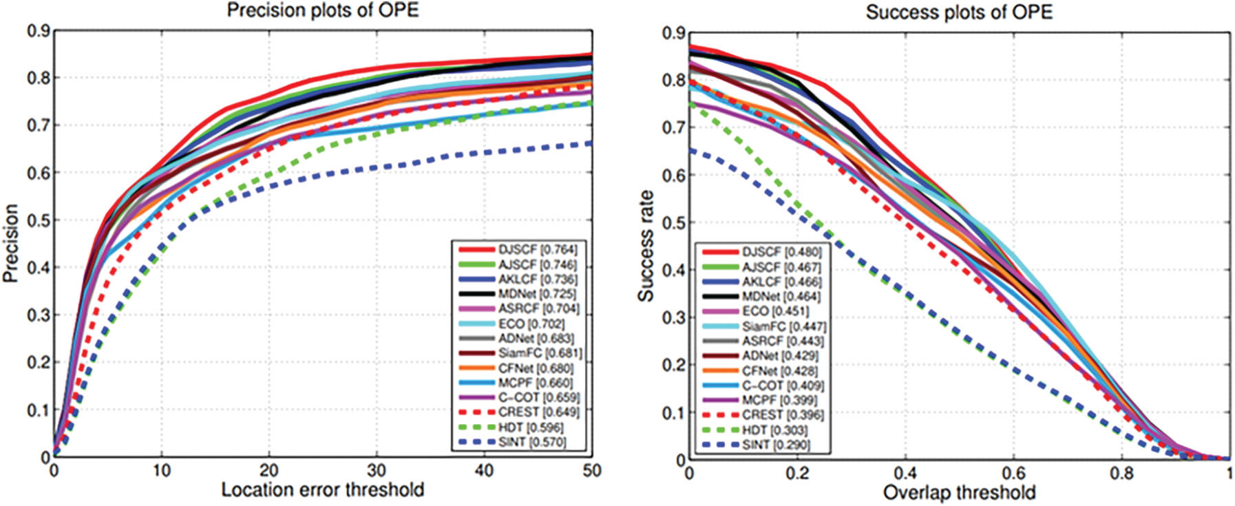
Figure 5: Comparison between DJSCF, AJSCF, and AKLCF trackers and different state-of-the-art deep-based trackers. The value of average precision and average success rate is calculated by OPE results from dataset UAVDT-S
To better demonstrate the superiority of our model in tracking performance, we selected 4 sets of video sequences in the DTB70 dataset to show the performance of the proposed method. As shown in Fig. 6, the different methods in each frame of the image The target tracking results are represented by different colored frames, which are ARCF-HC (red), LADCF (green), AKLCF (blue), DJSCF (black), and STRCF (pink). Because the target of UAV tracking is small, it is difficult to maintain a good tracking effect. For example, in Figs. 6a, 6d, the LADCF has a serious tracking offset, resulting in tracking failure, and STRCF also has the problem of expanding the tracking area in the Bike video. In short, our methods have always maintained a good tracking effect, and the tracking frame always surrounds the tracking target.
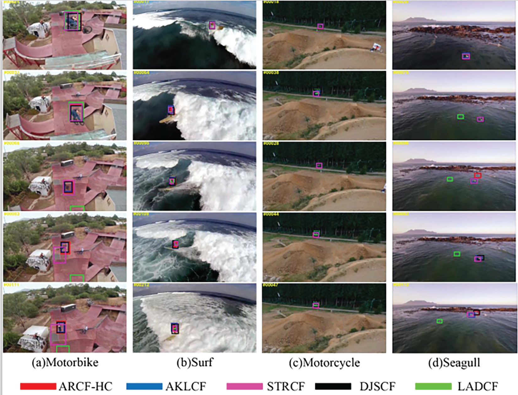
Figure 6: Comparison of tracking performance on the DTB70 dataset
To study the influence of parameter setting on the tracking effect, we carried out a corrosion analysis on the main parameters of the weighting matrix and obtained the parameter setting with the best tracking effect. Because there are two weighting matrices, namely two variable parameters
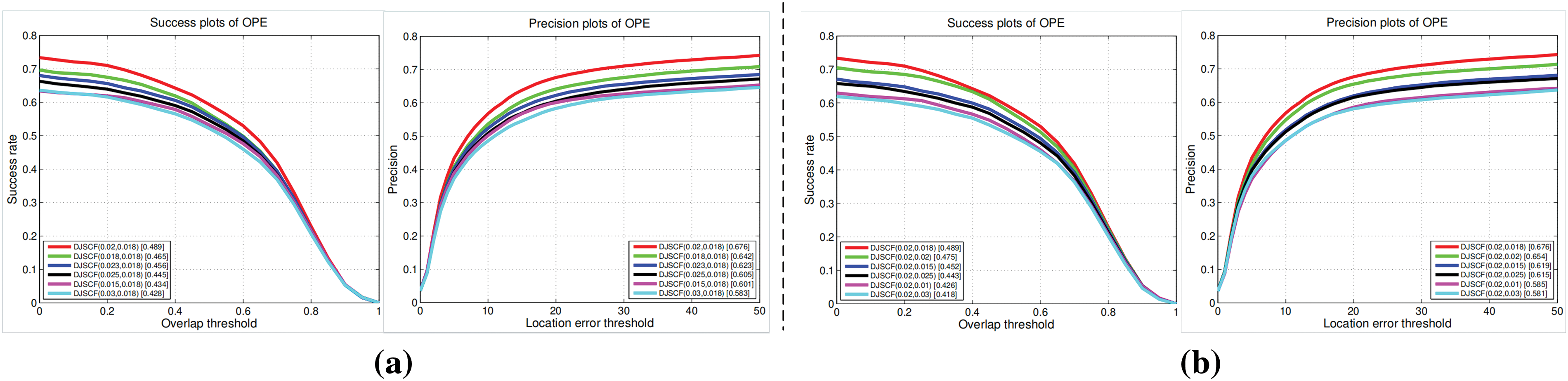
Figure 7: Comparison of tracking results based on different parameters
To reflect the superior robustness of DJSCF, we conducted comparative experiments between DJSCF, ARCF, and AKLCF based on the motorbike video sequence in the DTB70 dataset. As shown in Fig. 8, the robustness of the tracker is mainly reflected by the overlap rate of the target frame estimated by the model and the initial target frame in different frames of images and the overlap value shown on the ordinate. Among them, the blue line represents the ARCF tracker, and the red and green line represents the AKLCF and DJSCF, respectively. It can be seen from Fig. 8 that the overlap rate of DJSCF in different frames is higher than the other two, especially between 31 and 51 frames. This shows that although ARCF or AKLCF are affected by a complex environment and reduce the tracking effect, DJSCF can still maintain a high tracking accuracy and demonstrate good robustness.
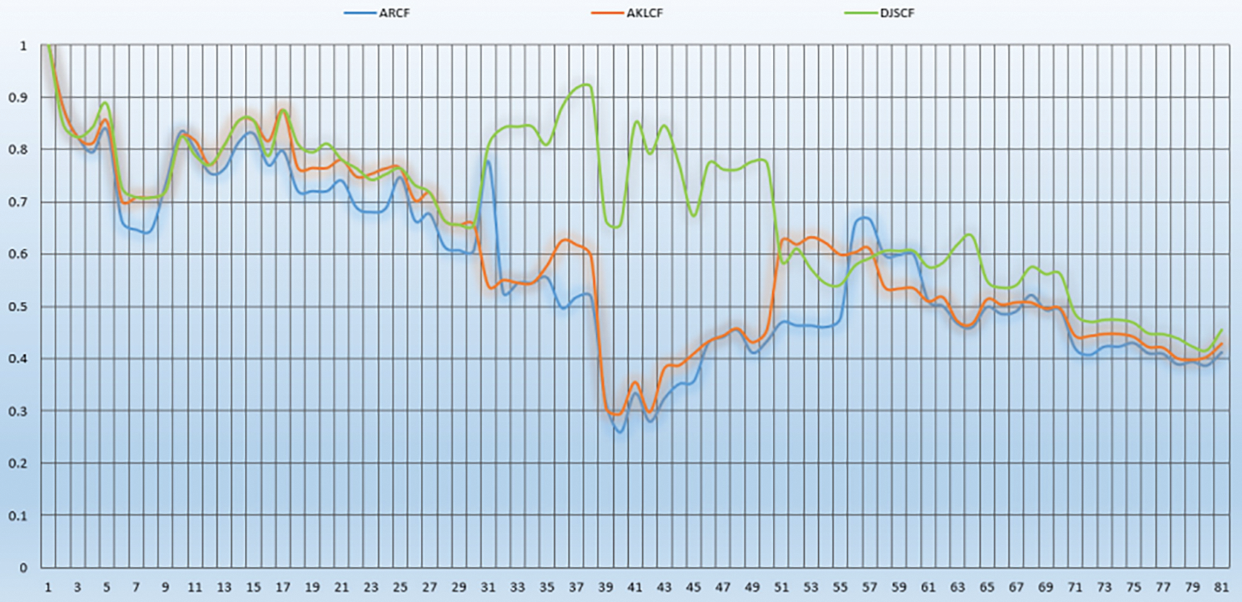
Figure 8: Comparison of robustness on the motorbike video sequence in the DTB70 dataset
To solve the distortion problem of correlation filter caused by boundary effect and background noise, this paper proposes a distorted KL dispersion correlation filter model by introducing KL dispersion, which improves the Euclidean distance of the original model and reduces the tracking offset caused by distortion caused by noise in the filter. In addition, a filter model of JS divergence correlation is proposed based on the two-domain weighted constraint. A large number of experimental results show that the proposed method can improve the accuracy of UAV video target tracking with less speed loss. However, due to the complexity of the DJSCF algorithm, the real-time requirements will be limited. In future work, adding convolution or depth network to the model may further improve the precision and success rate.
Acknowledgement: Resources and computing environment provided by Nanjing University of Posts and Telecommunications, Nanjing, China, thanks to the support of the school.
Funding Statement: This work is supported by the National Natural Science Foundation of China under Grant 62072256 and Natural Science Foundation of Nanjing University of Posts and Telecommunications (Grant Nos. NY221057 and NY220003).
Author Contributions: The authors confirm contribution to the paper as follows: study conception and design: Taiyu Yan, Guoxia Xu and Xiaoran Zhao; data collection: Yuxin Cao and Xiaoran Zhao; analysis and interpretation of results: Taiyu Yan, Guoxia Xu and Hu Zhu; draft manuscript preparation: Taiyu Yan, Yuxin Cao and Lizhen Deng. All authors reviewed the results and approved the final version of the manuscript.
Availability of Data and Materials: All code, dataset images, and other accessible materials in this article can be obtained through the email address of the corresponding author.
Conflicts of Interest: The authors declare that they have no conflicts of interest to report regarding the present study.
References
1. F. Wang, G. S. Li, Y. L. Wang, R. Wajid, Khosravi et al., “Privacy-aware traffic flowprediction based on multi-party sensor data with zero trust in smart city,” ACM Transactions on Internet Technology, 2022. https://doi.org/10.1145/3511904 [Google Scholar] [CrossRef]
2. Y. Chen, F. J. Zhao, X. Chen and Y. Wu, “Efficient multi-vehicle task offloading for mobile edge computing in 6 G networks,” IEEE Transactions on Vehicular Technology, vol. 71, no. 5, pp. 4584–4595, 2021. [Google Scholar]
3. L. Qi, W. Lin, X. Zhang, W. Dou, X. Xu et al., “A correlation graph based approach for personalized and compatible web APIs recommendation in mobile APP development,” IEEE Transactions on Knowledge and Data Engineering, vol. 35, no. 6, pp. 5444–5457, 2022. https://doi.org/10.1109/TKDE.2022.3168611 [Google Scholar] [CrossRef]
4. Y. Z. Xia, X. J. Deng, L. Z. Yi, L. T. Yang, X. Tang et al., “AI-driven and MEC-empowered confident information coverage hole recovery in 6G-enabled IoT,” IEEE Transactions on Network Science and Engineering, vol. 10, no. 3, pp. 1256–1269, 2022. https://doi.org/10.1109/TNSE.2022.3154760 [Google Scholar] [CrossRef]
5. J. W. Huang, Z. Y. Tong and Z. H. Feng, “Geographical POI recommendation for Internet of Things: A federated learning approach using matrix factorization,” International Journal of Communication Systems, pp. e5161, 2022. [Google Scholar]
6. A. Al-Mansor, N. Noordin, A. Saif and S. Alsamhi, “D2D multi-hop energy efficiency toward EMS in B5G,” in Proc. of Emerging Smart Technologies and Applications (eSmarTA), Ibb, Yemen, pp. 1–6, 2022. [Google Scholar]
7. Y. Chen, G. Wei and K. X. Li, “Dynamic task offloading for internet of things in mobile edge computing via deep reinforcement learning,” International Journal of Communication Systems, pp. e5154, 2022. [Google Scholar]
8. J. Huang, H. Gao, S. Wan and Y. Chen, “AoI-aware energy control and computation offloading for industrial IoT,” Future Generation Computer Systems, vol. 139, pp. 29–37, 2023. [Google Scholar]
9. Y. Liu, Z. Song, X. Xu, R. Wajid, X. Zhang et al., “Bidirectional GRU networks-based next POI category prediction for healthcare,” International Journal of Intelligent Systems, vol. 37, no. 7, pp. 4020–4040, 2022. [Google Scholar]
10. Y. Yang, X. Yang, M. H. Heidari, K. M. Ayoub, G. Srivastava et al., “ASTREAM: Data-stream-driven scalable anomaly detection with accuracy guarantee in IIoT environment,” IEEE Transactions on Network Science and Engineering, vol. 10, no. 5, pp. 3007–3016, 2022. https://doi.org/10.1109/TNSE.2022.3157730 [Google Scholar] [CrossRef]
11. Y. Chen, F. Zhao, Y. Lu and X. Chen, “Dynamic task offloading for mobile edge computing with hybrid energy supply,” Tsinghua Science and Technology, vol. 28, no. 3, pp. 421–432, 2023. https://doi.org/10.26599/TST.2021.9010050 [Google Scholar] [CrossRef]
12. L. Kong, L. Wang, W. Gong, C. Yan, Y. Duan et al., “LSH-aware multitype health data prediction with privacy preservation in edge environment,” World Wide Web, vol. 25, no. 5, pp. 1793–1808, 2022. [Google Scholar]
13. A. Saif, K. Dimyati, K. A. Noordin, S. H. Alsamhi, N. A. Mosali et al., “UAV and relay cooperation based on RSS for extending smart environments coverage area in B5G,” 2022. https://doi.org/10.21203/rs.3.rs-2002265/v1 [Google Scholar] [CrossRef]
14. C. Xu, G. Zheng and X. Zhao, “Energy-minimization task offloading and resource allocation for mobile edge computing in NOMA heterogeneous networks,” IEEE Transactions on Vehicular Technology, vol. 69, no. 12, pp. 16001–16016, 2020. [Google Scholar]
15. L. Qi, Y. Liu, Y. Zhang, X. Xu, M. Bilal et al., “Privacy-aware point-of-interest category recommendation in Internet of Things,” IEEE Internet of Things Journal, vol. 9, no. 21, pp. 21398–21408, 2022. [Google Scholar]
16. Y. W. Liu, D. J. Li, S. H. Wan, F. Wang, W. Dou et al., “Along short-term memory-based model for greenhouse climate prediction,” International Journal of Intelligent Systems, vol. 37, no. 1, pp. 135–151, 2022. [Google Scholar]
17. L. Qi, Y. Yang, X. Zhou, W. Rafique and J. Ma, “Fast anomaly identification based on multiaspect data streams for intelligent intrusion detection toward secure Industry 4.0,” IEEE Transactions on Industrial Informatics, vol. 18, no. 9, pp. 6503–6511, 2022. [Google Scholar]
18. K. Li, J. Zhao, J. Hu and Y. Chen, “Dynamic energy efficient task offloading and resource allocation for noma-enabled IoT in smart buildings and environment,” Building and Environment, vol. 226, pp. 109513, 2022. [Google Scholar]
19. J. Xu, D. Li and W. Gu, “UAV-assisted task offloading for IoT in smart buildings and environment via deep reinforcement learning,” Building and Environment, vol. 222, pp. 109218, 2022. [Google Scholar]
20. M. Li, N. Cheng, J. Gao, Y. Wang, L. Zhao et al., “Energy-efficient UAV-assisted mobile edge computing: Resource allocation and trajectory optimization,” IEEE Transactions on Vehicular Technology, vol. 69, no. 3, pp. 3424–3438, 2020. [Google Scholar]
21. Y. Yin, X. Wang, D. Xu, F. Liu, Y. Wang et al., “Robust visual detection–learning–tracking framework for autonomous aerial refueling of UAVs,” IEEE Transactions on Instrumentation and Measurement, vol. 65, no. 3, pp. 510–521, 2016. [Google Scholar]
22. N. Liang, G. Wu, W. Kang, Z. Wang and D. D. Feng, “Real-time long-term tracking with prediction-detection-correction,” IEEE Transactions on Multimedia, vol. 20, no. 9, pp. 2289–2302, 2018. [Google Scholar]
23. H. Cheng, L. Lin, Z. Zheng, Y. Guan and Z. Liu, “An autonomous vision-based target tracking system for rotorcraft unmanned aerial vehicles,” in 2017 IEEE/RSJ Int. Conf. on Intelligent Robots and Systems, Vancouver, Canada, pp. 1732–1738, 2017. [Google Scholar]
24. G. Xu, H. Wang, M. Zhao, M. Pedersen and H. Zhu, “Learning the distribution-based temporal knowledge with low rank response reasoning for UAV visual tracking,” IEEE Transactions on Intelligent Transportation Systems, pp. 1–11, 2022. https://doi.org/10.1109/TITS.2022.3200829 [Google Scholar] [CrossRef]
25. F. Wang, H. Zhu, G. Srivastava, S. Li, M. R. Khosravi et al., “Robust collaborative filtering recommendation with user-item-trust records,” IEEE Transactions on Computational Social Systems, vol. 9, no. 4, pp. 986–996, 2022. [Google Scholar]
26. Y. Wu, J. Lim and M. H. Yang, “Object tracking benchmark,” IEEE Transactions on Pattern Analysis and Machine Intelligence, vol. 37, no. 9, pp. 1834–1848, 2015. [Google Scholar] [PubMed]
27. M. Kristan, J. Matas, A. Leonardis, M. Felsberg, L. Cehovin et al., “The visual object tracking VOT2015 challenge results,” in Proc. of CVPR, Boston, MA, USA, pp. 564–586, 2015. [Google Scholar]
28. M. Kristan, R. Pflugfelder and J. Matas, “The visual object tracking VOT2016 challenge results,” in Proc. of ECCV, Amsterdam, NL, pp. 777–824, 2016. [Google Scholar]
29. S. Li and D. Yeung, “Visual object tracking for unmanned aerial vehicles: A benchmark and new motion models,” in Proc. of AAAI, San Francisco, CA, USA, pp. 4140–4146, 2017. [Google Scholar]
30. D. Du, Y. Qi, H. Yu, Y. Yang, K. Duan et al., “The unmanned aerial vehicle benchmark: Object detection and tracking,” in Proc. of ECCV, Munich, Germany, pp. 370–386, 2018. [Google Scholar]
31. M. Danelljan, G. Hager, F. S. Khan and M. Felsberg, “Learning spatially regularized correlation filters for visual tracking,” in Proc. of ICCV, Santiago, Chile, pp. 4310–4318, 2015. [Google Scholar]
32. F. Li, C. Tian, W. Zuo, L. Zhang and M. H. Yang, “Learning spatial-temporal regularized correlation filters for visual tracking,” in Proc. of CVPR, Salt Lake City, UT, USA, pp. 4904–4913, 2018. [Google Scholar]
33. K. Dai, D. Wang, H. C. Lu, C. Sun and J. H. Li, “Visual tracking via adaptive spatially-regularized correlation filters,” in Proc. of CVPR, Long Beach, CA, USA, pp. 4665–4674, 2019. [Google Scholar]
34. H. K. Galoogahi, A. Fagg and S. Lucey, “Learning background-aware correlation filters for visual tracking,” in Proc. of ICCV, Venice, Italy, pp. 1144–1152, 2017. [Google Scholar]
35. T. Xu, Z. Feng, X. Wu and J. Kittler, “Joint group feature selection and discriminative filter learning for robust visual object tracking,” in Proc. of ICCV, Seoul, Korea, pp. 7949–7959, 2019. [Google Scholar]
36. H. Zhu, H. Ni, S. Liu, G. Xu and L. Deng, “TNLRS: Target-aware non-local low-rank modeling with saliency filtering regularization for infrared small target detection,” IEEE Transactions on Image Processing, vol. 29, pp. 9546–9558, 2020. [Google Scholar]
37. M. Wang, Y. Liu and Z. Huang, “Large margin object tracking with circulant feature maps,” in Proc. of CVPR, Honolulu, HI, USA, pp. 4021–4029, 2017. [Google Scholar]
38. J. Choi, H. Chang, S. Yun, T. Fischer, Y. Demiris et al., “Attentional correlation filter network for adaptive visual tracking,” in Proc. of CVPR, Honolulu, HI, USA, pp. 4807–4816, 2017. [Google Scholar]
39. Z. Huang, C. Fu, Y. Li, F. Lin and P. Lu, “Learning aberrance repressed correlation filters for real-time UAV tracking,” in Proc. of ICCV, Seoul, Korea, pp. 2891–2900, 2019. [Google Scholar]
40. F. Li, X. H. Wu, W. M. Zuo, D. Zhang and L. Zhang, “Remove cosine window from correlation filter-based visual trackers: When and how,” IEEE Transactions on Image Processing, vol. 29, no. 99, pp. 1, 2020. [Google Scholar]
41. X. Xue, Y. Li, X. Yin, C. Shang, T. Peng et al., “Semantic-aware real-time correlation tracking framework for UAV videos,” IEEE Transactions on Cybernetics, vol. 52, pp. 1–12, 2020. [Google Scholar]
42. C. Fu, Y. Zhang, Z. Huang, R. Duan and Z. Xie, “Part-based background-aware tracking for UAV with convolutional features,” IEEE Access, vol. 7, pp. 79997–80010, 2019. [Google Scholar]
43. Y. Li, C. Fu, F. Ding, Z. Huang and G. Lu, “Autotrack: Towards high-performance visual trac for UAV with automatic spatio-temporal regularization,” in Proc. of CVPR, Washington DC, USA, pp. 11920–11929, 2020. [Google Scholar]
44. G. Xu, X. Deng, X. Zhou, M. Pedersen, L. Cimmino et al., “FCFusion: Fractal componentwise modeling with group sparsity for medical image fusion,” IEEE Transactions on Industrial Informatics, vol. 18, no. 12, pp. 9141–9150, 2022. [Google Scholar]
45. M. Danelljan, L. V. Gool and R. Timofte, “Probabilistic regression for visual tracking,” in Proc. of CVPR, Washington DC, USA, pp. 7183–7192, 2020. [Google Scholar]
46. B. Barz, E. Rodner, Y. G. Garcia and J. Denzler, “Detecting regions of maximal divergence for spatio-temporal anomaly detection,” IEEE Transactions on Pattern Analysis and Machine Intelligence, vol. 41, no. 5, pp. 1088–1101, 2019. [Google Scholar] [PubMed]
47. M. Jiang, A. Beutel, P. Cui, B. Hooi, S. Yang et al., “A general suspiciousness metric for dense blocks in multimodal data,” in Proc. of ICDM, Atlantic City, NJ, USA, pp. 781–786, 2015. [Google Scholar]
48. V. Roth, “Outlier detection with one-class kernel fisher discriminants,” Advances in Neural Information Processing Systems, vol. 17, pp. 1169–1176, 2004. [Google Scholar]
49. J. F. Henriques, C. Rui, P. Martins and J. Batista, “Exploiting the circulant structure of tracking-by-detection with kernels,” in Proc. of ECCV, Florence, Italy, pp. 702–715, 2012. [Google Scholar]
50. S. Tan, J. Jiao and W. Zheng, “Weakly supervised open-set domain adaptation by dual-domain collaboration,” in Proc. of CVPR, Long Beach, CA, USA, pp. 5389–5398, 2019. [Google Scholar]
51. J. Xu, L. Zhang and D. Zhang, “A trilateral weighted sparse coding scheme for real-world image denoising,” in Proc. of ECCV, Munich, Germany, pp. 21–38, 2018. [Google Scholar]
52. T. Xu, Z. Feng, X. Wu and J. Kittler, “Learning adaptive discriminative correlation filters via temporal consistency preserving spatial feature selection for robust visual object tracking,” IEEE Transactions on Image Processing, vol. 28, no. 11, pp. 5596–5609, 2019. [Google Scholar] [PubMed]
53. Y. Yang, H. T. Shen, Z. Ma, Z. Huang and X. Zhou, “L2, 1-norm regularized discriminative feature selection for unsupervised learning,” in Proc. of IJCAI, Barcelona, Spain, pp. 1589, 2011. [Google Scholar]
54. K. Simonyan and A. Zisserman, “Very deep convolutional networks for large-scale image recognition,” in 3rd Int. Conf. on Learning Representations, ICLR 2015, San Diego, CA, USA, 2015. [Online]. Available: http://arxiv.org/abs/1409.1556 [Google Scholar]
55. M. Mueller, N. Smith and B. Ghanem, “A benchmark and simulator for UAV tracking,” in Proc. of ECCV, Amsterdam, Nederland, pp. 445–461, 2016. [Google Scholar]
56. L. Wen, P. Zhu, D. Du, X. Bian, H. Ling et al., “Visdrone-sot2018: The vision meets drone single-object tracking challenge results,” in Proc. of ECCV, Munich, Germany, pp. 1–27, 2018. [Google Scholar]
57. Y. Wu, J. Lim and M. H. Yang, “Online object tracking: A benchmark,” in Proc. of CVPR, Portland, OR, USA, pp. 2411–2418, 2013. [Google Scholar]
58. M. Danelljan, G. Hager, F. Khan and M. Felsberg, “Accurate scale estimation for robust visual tracking,” in Proc. of BMVC, Nottingham, UK, pp. 254–265, 2014. [Google Scholar]
59. Y. Li and J. Zhu, “A scale adaptive kernel correlation filter tracker with feature integration,” in Proc. of ECCV, Zurich, Switzerland, pp. 254–265, 2014. [Google Scholar]
60. M. Danelljan, G. Bhat, F. S. Khan and M. Felsberg, “ECO: Efcient convolution operators for tracking,” in Proc. of CVPR, Honolulu, HI, USA, pp. 6931–6939, 2017. [Google Scholar]
61. C. Ma, J. B. Huang, X. Yang and M. H. Yang, “Hierarchical convolutional features for visual tracking,” in Proc. of CVPR, Boston, MA, USA, pp. 1–6, 2015. [Google Scholar]
62. M. Danelljan, A. Robinson, F. Khan and M. Felsberg, “Beyond correlation filters: Learning continuous convolution operators for visual tracking,” in Proc. of CVPR, Las Vegas, NV, USA, pp. 472–488, 2016. [Google Scholar]
63. H. Nam and B. Han, “Learning multi-domain convolutional neural networks for visual tracking,” in Proc. of CVPR, Las Vegas, NV, USA, pp. 4293–4302, 2016. [Google Scholar]
64. S. Yun, J. Choi, Y. Yoo, K. Yun and J. Y. Choi, “Action-decision networks for visual tracking with deep reinforcement learning,” in Proc. of CVPR, Honolulu, HI, USA, pp. 2711–2720, 2017. [Google Scholar]
65. J. Valmadre, L. Bertinetto, J. Henriques, A. Vedaldi and P. H. Torr, “End-to-end representation learning for correlation filter based tracking,” in Proc. of CVPR, Honolulu, HI, USA, pp. 5000–5008, 2017. [Google Scholar]
66. Y. Song, C. Ma, L. Gong, J. Zhang, R. W. H. Lau et al., “Convolutional residual learning for visual tracking,” in Proc. of CVPR, Honolulu, HI, USA, pp. 2555–2564, 2017. [Google Scholar]
67. T. Zhang, C. Xu and M. Yang, “Multi-task correlation particle filter for robust object tracking,” in Proc. of CVPR, Honolulu, HI, USA, pp. 4335–4343, 2017. [Google Scholar]
68. L. Bertinetto, J. Valmadre, J. F. Henriques, A. Vedaldi and P. H. Torr, “Fully-convolutional siamese networks for object tracking,” in Proc. of ECCV, Tel-Aviv, Amsterdam, Nederland, pp. 850–865, 2016. [Google Scholar]
69. Y. Qi, S. Zhang, L. Qin, H. Yao, Q. Huang et al., “Hedged deep tracking,” in Proc. of CVPR, Las Vegas, NV, USA, pp. 2–6, 2016. [Google Scholar]
Cite This Article
 Copyright © 2023 The Author(s). Published by Tech Science Press.
This work is licensed under a Creative Commons Attribution 4.0 International License , which permits unrestricted use, distribution, and reproduction in any medium, provided the original work is properly cited.
 Downloads
 Citation Tools