DNEF: A New Ensemble Framework Based on Deep Network Structure

1  Introduction

Nowadays, machine learning and artificial intelligence have been applied to various fields with remarkable success. Ensemble learning is of great interest among machine learning and Artificial intelligence methods, because of its ability to combine numerous learners to achieve significantly improving the accuracy and generalization performance of the model. Dietterich demonstrated the performance advantages of ensemble learning over a single classifier in statistical, computational, and representational ways [1]. In addition, base classifiers in the ensemble model are typically weak classifiers, which are more trainable than a single strong classifier.

The main challenges in designing ensemble models are the diversity of sub-learners and the ensemble strategies. (1) The diversity of sub-learners: diversity prompts the provision of complementary information among sub-learners [2] and is more advantageous in improving the performance of the ensemble model [3]. To maintain the diversity of sub-learners, most ensemble algorithms construct different types of sub-learners on the same instance space or the same type of sub-learners on different instance space (e.g., ensemble methods based on bagging, including Random Forest (RF) [4], Bagging of Extrapolation Borderline-SMOTE SVM (BEBS) [5], etc...) (2) Ensemble strategies for base classifiers. Typical ensemble strategies include boosting [6] and the base classifier weight-based strategy. Boosting methods improve the classification ability of misclassified instances by adjusting the instance weights to obtain a higher performance of the ensemble model. The sub-classifier weight-based strategy improves the performance of the ensemble model by adjusting the weights of the base classifiers.

Traditional algorithms often adopt a single strategy, ignoring the complex representation of the ensemble model. In this paper, we propose the Deep Network Ensemble Framework (DNEF), which draws on the concept of deep learning and the structure of the neural network. The DNEF framework adopts a hierarchical network structure that combines various ensemble strategies to improve both the diversity of base classifiers and the generalization ability of the ensemble framework. The novelty of the proposed DNEF includes: (1) Construction of different types of base classifiers on various instance subspaces to maximize the diversity of base classifiers in the hidden layer. (2) Combining the boost ensemble strategy and the metric-based ensemble strategy to optimize instance distribution, improve generalization capability, determine base classifier weights, and transfer misclassified instances between the hidden layers. (3) Adoption of an intra-layer parallel inter-layer serial training model to enhance training efficiency. (4) Comparative experiments show that our proposed DNEF achieves significant improvement in classification accuracy compared to popular ensemble algorithms.

2  Related Works

Our approach is related to ensemble learning. We briefly describe the related work including the present ensemble learning and deep ensemble learning in the following sub-sections.

2.1 Traditional Ensemble Learning

Ensemble learning is one of the highly effective learning algorithms in machine learning. The procedure of ensemble learning involves combining multiple weak learners according to a certain strategy into a strong learner with higher predictive performance [7]. Compared to individual algorithms, it has been found that ensemble learning could combine the advantages of each weak learner to represent complex models more accurately, reducing overfitting and providing higher learning performance. Thus, ensemble learning has a wide range of applications for complex data models such as loan approval [8], speech recognition [9], image recognition [10], and industrial process simulation [11].

As mentioned above, the main challenges in designing ensemble models are the diversity of base classifiers and the ensemble strategy. Several typical Ensemble Learning models are described below.

2.1.1 Random Forest

Random Forest is a model for classification and regression that combines the “bagging” method with random feature selection. Random Forest employs the bagging method to select instances to train different random decision trees, which are then combined based on an ensemble strategy.

Current improvements to Random Forest have focused on increasing the diversity of the trees by adding random factors (Menze [12], Zhang et al. [13–15]) and on designing ensemble strategies. For example, Utkin et al. proposed optimizing weights in terms of forest accuracy [16,17]. Random Forest has been widely used in different classification scenarios in recent years. In the industrial scenario, Paul et al. used the improved Random Forest for the classification of dual-phase (DP) steel microstructures [18]. In Intrusion Detection Systems, Resende et al. proposed that the Random Forest has the advantage of speed and efficiency over common machine learning methods [19].

2.1.2 AdaBoost

AdaBoost [20] is a highly popular boosting learning algorithm for improving classification accuracy. It iteratively constructs multiple weak classifiers, with each classifier improving its performance by adjusting weights. During each iteration, AdaBoost increases the weights of the instances that were misclassified in the previous iteration, directing the classifier’s attention towards these instances in subsequent rounds, ultimately leading to higher accuracy. In the realm of chemical detection, Chen et al. found that AdaBoost can be used simultaneously to determine the trace copper and cobalt in high-concentration zinc solution [21]. In the field of electrocardiogram (ECG) classification, Barstuğan et al. employed AdaBoost as a classifier based on a dictionary, using it to classify ECG signals [22].

2.1.3 Stacking

Stacking [23–25] is a hierarchical ensemble learning framework. Stacking methods learn some base classifiers (usually, these learners are of different types) using the initial training data and employ the predictions generated by these base classifiers as a new training set to train a new classifier. Stacking can improve accuracy by reducing the bias in data. Stacking technology has made significant progress in a large number of areas of application. In mining engineering, Koopialipoor et al. predicted rock deformation using the structure of a stacked tree, Random Forest (RF), K-Nearest-Neighbors (KNN), and Multilayer Perceptron (MLP) [26]. For diabetes identification, Kalagotla et al. developed a novel stacking technique with a multi-layer perceptron, support vector machine, and logistic regression to predict diabetes [27].

2.1.4 Weighted-Based Voting

The voting strategy, as a decision rule, is important in ensemble learning. Typically, the predictions are made through majority voting. The voting strategy can be generally divided into weighted and unweighted voting. Among them, weighted voting is a commonly employed approach. Weighted voting can be further divided into dynamic weighted voting [28] and static weighted voting. Voting technology has become well-established in a variety of classification scenarios. In the domain of tuberculosis prediction, Okezie et al. used the weighted voting ensemble technique to improve the accuracy of tuberculosis diagnosis [29]. For Business failure prediction, Kim et al. used a majority voting ensemble method with a decision tree to predict business failure [30].

2.2 Deep Ensemble Learning

After the significant development of deep learning, there has been a widespread focus on how to combine deep learning and ensemble learning to leverage their advantages. Deep ensemble learning encompasses the design of ensemble models and fusion mechanisms. By aggregating multiple deep learning models, the hierarchical relationships between these models are used to achieve more powerful feature extraction and representation capabilities. In this section, we begin by introducing ensemble learning based on neural network modules, followed by an introduction to deep forest.

Sivakumar et al. proposed a deep learning-based graph neural network (DL-GNN) based on the ensemble of recurrent neural networks (RNN) and feedforward neural networks (FNN) [31]. Devarajan et al. introduced a deep learning model integrated with natural language processing (N-DCBL), which combines a convolutional neural network (CNN), Bidirectional Long Short-Term Memory (Bi-LSTM), and Attention [32]. José et al. presented an automated deep learning-based breast cancer diagnosis model (ADL-BCD) for breast cancer diagnosis using digital mammograms. ADL-BCD is an ensemble model of Gaussian filter (GF)-based preprocessing, Tsallis entropy-based segmentation, ResNet34 based feature extraction, chimp optimization algorithm (COA) based parameter tuning, and the wavelet neural network (WNN) based classification [33]. Hussain et al. developed an Ensemble Deep-Learning-Enabled Clinical Decision Support System for Breast Cancer Diagnosis (EDLCDS-BCD). The EDLCDS-BCDC ensemble of VGG-16, VGG-19, and SqueezeNet for feature extraction [34].

Zhou et al. [35] proposed the Deep Forest (DF) model, which is a multi-grained cascade structure. DF typically comprises two steps: the multi-grained scanner and the cascade forest. The former extracts information from raw data while the latter constructs an adaptive-depth ensemble model. DF is a model that combines ensemble learning and deep learning. On the one hand, it is an ensemble learning method based on the decision tree, inheriting most of the advantages of general ensemble learning methods. On the other hand, DF also has the advantages of deep neural networks to increase the diversity of ensemble learning and improve model performance. Subsequently, the deep forest methods have been improved, such as siamese deep forest [36], imprecise deep forest for classification [37], and applied to various domains, including software defect prediction, price prediction, prediction of protein interactions, anti-cancer drug response prediction [38–41].

2.3 Characteristics of DNEF

Our deep ensemble framework, DNEF, combines the structure of deep networks with ensemble learning. Specifically, we use a weighting strategy to facilitate the iteration of DNEF and a transfer strategy to ensure the architectural complexity of the DNEF. Popular ensemble models often employ a single strategy, such as RF, AdaBoost, etc., while DNEF employs two ensemble strategies: the weighting strategy and the transfer strategy. These two strategies take into account both the relationship between classifiers and the complexity of the ensemble structure. Compared to the deep ensemble models based on the neural network, DNEF does not incorporate deep learning modules and does not use neural networks and backpropagation. The weighting strategy in DNEF supports the iteration of the hidden layer, while the transfer strategy enhances the connectivity of the hidden layer. These key differences represent the biggest differentiating factor between DNEF and deep ensemble learning.

3  The Proposed Method

In this section, we introduce our proposed DNEF framework. We first describe the DNEF in Section 3.1. We then explain the weighting strategy and transfer strategy of DNEF in Section 3.2.

3.1 Introduction of DNEF

Inspired by deep neural networks, we propose the DNEF framework, which employs a deep network architecture. From Fig. 1, the DNEF framework includes an input layer, hidden layers, and an output layer. The data in the input layer consists of randomly sampled instances X0. The DNEF framework iterates between hidden layers based on a weighting strategy. Each hidden layer contains m nodes, and each node represents a base classifier h (in this paper, we use the decision tree as the base classifier). The inputs to the node are instances with their weights. In the hidden layer interior, each node generates transfer instances and corresponding weights based on the transfer strategy. These transfer instances and transfer instance weights of all nodes are aggregated with the input data to produce the output data of the next layer. The output of DNEF is obtained through a weighted ensemble of classifiers across all layers.

Figure 1: The architecture of DNEF

It is worth noting that the “ensemble” in this DNEF is based on a deep network structure. Two factors contribute to the accuracy and robustness of DNEF: Firstly, the hidden layer of DNEF builds more accurate base classifiers by utilizing the results of the previous layer. Secondly, independent classifiers are trained in parallel in the hidden layer to reduce variance.

It is also worth mentioning that the key issues are the calculation of instance weights and the transfer strategy that directly affect the performance of the DNEF. As one of the main contributions of this paper, we propose the weighting strategy and the transfer strategy.

The procedures for the weighting strategy and transfer strategy are described below:

1. The procedure of weighting strategy:

(1) Calculation of the base classifier weights Wc: We compute the weight of the base classifier based on its current class error e.

(2) Calculation of instance weights Ws: The instance weights Ws are calculated based on the Wc.

2. The procedure of transfer strategy:

(1) Selecting transfer instances X′ and transfer instance weights Ws′: We select transfer instances and their weights based on the size of training instances and the accuracy of the base classifiers.

(2) Transferring X′ with transfer instance weights Ws′ to the next layer: We Combine the transfer instances X′ of each base classifier with their weights Ws′ into the input data of each base classifier to form the output data. It should be noted that the input data of the base classifier does not include its own transfer instances andtransfer instance weights.

After describing the weighting strategy and the transfer strategy, we show the process of the DNEF framework. Each node in the input layer receives randomly sampled data D0j as its input:

D0j={(X0j,y),W0js},X0j∼X,W0js=1,j=1,2,⋯,m(1)

D0={D01,⋯,D0m}(2)

where X∈Rn, X0j represents the training instances of j-th node in the input layer, W0js is the instance weights of X0j and y represents the labels of instances y∈𝒴={1,−1}. m represents the total number of nodes in the hidden layer. D0 represents the input data of the input layer.

In the i-th hidden layer, Dij represents the training data of the j-th node. The weights Wic of base classifiersare calculated using the weighting strategy. The training data Di+1 of the next hidden layer are generated according to the transfer strategy.

Di={Di1,⋯,Dim}(3)

Dij={(Xij,y),Wijs}(4)

where Xij represents the training instances of j-th node in the i-th layer, Wijs is the instance weights of Xij.

The output of DNEF f is to ensemble the base classifiers H with weights Wc that were trained by the deep network structure.

f(X)=sign(∑i∑jHij∗Wijc(X))(5)

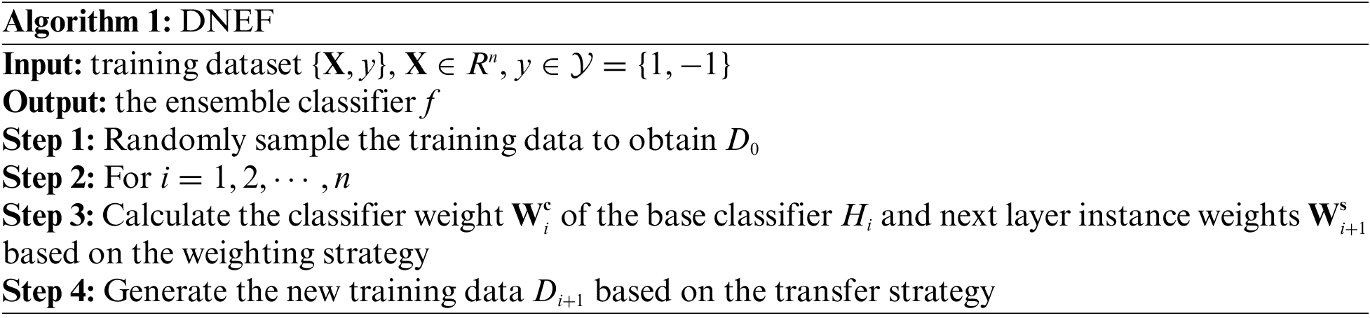
Algorithm 1 gives the process of DNEF, which combines the weighting strategy and the transfer strategy in hidden layers.

3.2 The Strategies of DNEF

In this section, we illustrate the two main strategies of the proposed DNEF framework. In Section 3.2.1, we explain the weighting strategy for the DNEF, followed by a description of the transfer strategy in Section 3.2.2.

3.2.1 DNEF’s Weighting Strategy

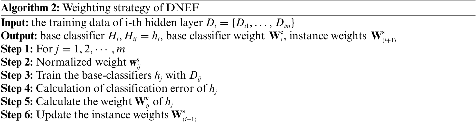
In this subsection, we describe the weighting strategy used in the DNEF framework. Firstly, given the training data for the j-th node in the i-th hidden layer Dij, The base classifier hj is trained using the instances Xij, with each instance being assigned the weights Wijs. Next, the instance weights W(i+1)js are calculated based on the classifier error e. The computing procedure of these weights is as follows: 1. Base classifier weight Wijc; 2. Instance weights W(i+1)js. Algorithm 2 illustrates the weighting strategy employed by the DNEF in the i-th hidden layer.

We first normalize the instance weights:

Wij,ks=wij,ks∑kwij,ks,k=1,2,3…,l(6)

where wij,ks is the k-th of wijs. l is the size of the instance weights wijs.

Then, the error e of the base classifier is calculated based on the classification result of the classifier hj.

e=∑kwij,ksI[y≠hj(Xij,k)](7)

where Xij,k is the k-th instance of Xij. I[y≠hj(Xij,k)] is defined as:

I[y≠hj(Xij,k)]={1hj(Xij,k)≠y0hj(Xij,k)=y(8)

The base classifier weight of hj is expressed as Wijc:

Wijc={12ln⁡(1−e)/e+αγe<=γ12ln⁡(1−e)/ee>γ(9)

where γ is the threshold value we set. αγ is a constant needed so that the equation is continuous [42].

αγ=12ln⁡(1−γγ)−12ln⁡(1−γγ)(10)

When considering the weight of hj, the higher-performing base classifier should have a larger weight. Therefore, we use the square root function to scale the weights of oversized classifiers:

12ln⁡((1−e)/e)+αγ(11)

After calculating the classifier weights Wijc, we update the instance weights W(i+1)js as follows:

W(i+1)js=Wijsexp⁡(Wijc∗I[y≠hj(Xij)])(12)

where Wijc helps to adjust the ensemble weights of the base classifier, W(i+1)js preserves the processing results of the previous layer as the input of the next layer.

3.2.2 The Adaptive Transfer Strategy in DNEF

We design a rule for the base classifier to adaptively choose transfer instances X′ and transfer instance weights Ws′. We then add transfer instances X′ with their weights Ws′ to the input as output data.

In the i-th hidden layer, we use parameters ε and μ to adaptively select the transfer weights W(i+1)s′ (see Algorithm 3). Here ε denotes the accuracy threshold, and μ denotes the instance size threshold. Under the control ε followed by μ, we select a portion of W(i+1)js as the transfer weight W(i+1)js′ in the j-th node. These weights are then assigned to the corresponding instances, forming the transfer instance X(i+1)j′.

Next, we aggregate all the transfer instances X(i+1)j′ with instances Xij of the j-th node.

X(i+1)j=(Xij,Xi1′,…,Xi(j−1)′,Xi(j+1)′,…,Xim′)(13)

Additionally, we aggregate all the transfer instance weights W(i+1)js′ with the instance weights W(i+1)js of j-th node.

W(i+1)js=(W(i+1)js,W(i+1)1s′,…,W(i+1)(j−1)s′,W(i+1)(j+1)s′,…,W(i+1)ms′)(14)

The new training data D(i+1)j is obtained:

D(i+1)j={(X(i+1)j,y),W(i+1)js}(15)

We obtain Di+1 by executing the transfer strategy on all nodes of the i-th hidden layer.

Di+1={D(i+1)1,…,D(i+1)m}(16)

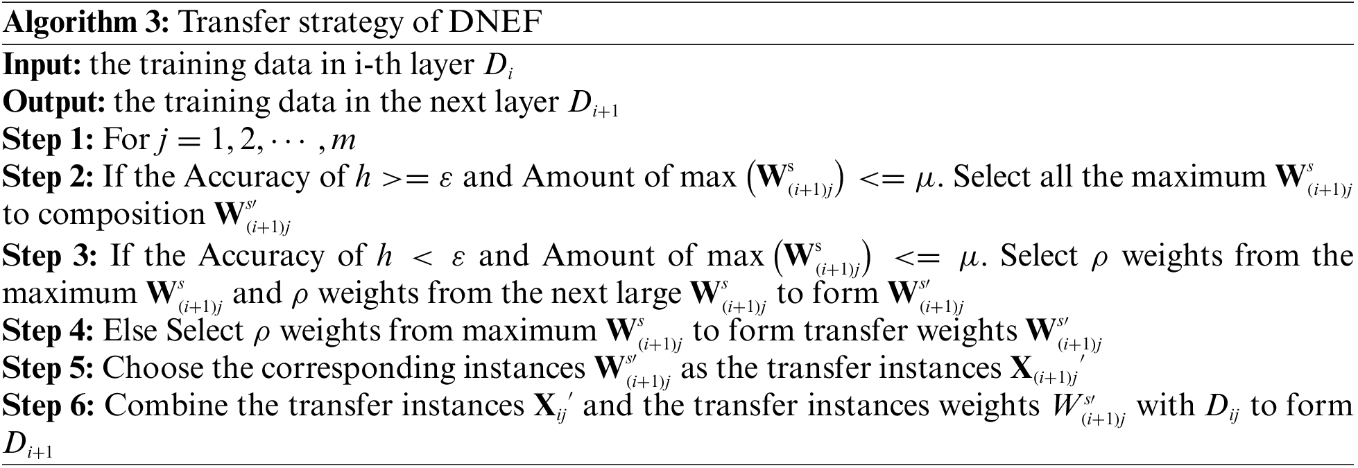
The transfer strategy dynamically selects the misclassified instances with weights into the next layer of training data. Algorithm 3 describes the transfer strategy.

4  Experiments

The experimental environment used in this study consisted of an Intel(R) Xeon(R) CPU E5-2640 v3 and Tesla K80 GPU 11 GB memory. All the experiments were conducted in a Python environment. The required Python libraries for carrying out the experiments were Sklearn, Numpy, Pandas, and Pytorch. The selected methods for providing comparison results included DNEF, Random Forest (RF), AdaBoost, Linear Support Vector Machine (SVM), MLP, and Voting (Decision Tree).

4.1 Datasets

The performance of the DNEF was validated using four datasets of varying dimensions. The Adult dataset has 14 features, the REJAFADA dataset with 6824 features, the Segmentation dataset has 19 features, and the IMDB dataset has 74849 features. We downloaded the Adult dataset, REJAFADA, and Segmentation datasets from the UCI machine learning repository and the IMDB dataset from the Stanford repository.

Table 1 gives the class, instance size, and dimensional information of these datasets.

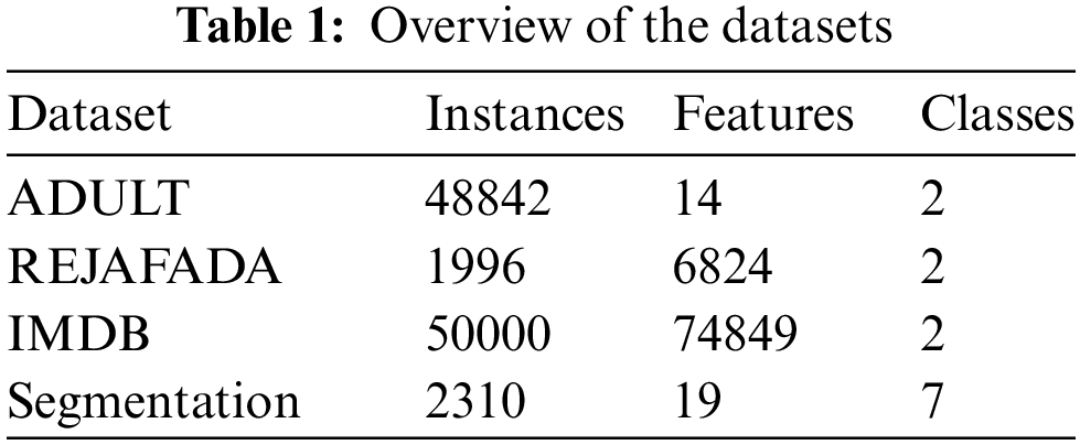
The ADULT dataset comprises 14 features and 48842 instances. The problem is to classify whether the income exceeds $50K/year.

The REJAFADA dataset contains 6824 features and 1996 instances. The problem it addresses is classifying files between benign and malware.

The IMDB dataset with 74849 features and 50,000 instances. The IMDB dataset is represented by tf-idf features with positive and negative labels.

The Segmentation dataset consists of 19 features and 2310 instances. Its objective is to classify seven distinct scenarios.

4.2 Experimental Settings

All results for each model were calculated using the same data set and random seeds for the metrics. The DNEF was set up as follows: (1) Each hidden layer consisted of three nodes. (2) The thresholds γ, ε, μ and ρ of DNEF were set at 0.15%, 0.9%, 150%, and 10%. Here, γ represents the threshold for base classifier error, ε represents the threshold for accuracy, μ represents the threshold for instance size and µ represents the percentage of the transfer weights. The base classifier in DNEF can be any classification model with instance weights. To ensure fairness in our evaluation, we employed the same decision tree as RF, AdaBoost, and Voting for the base classifier of DNEF. The parameters for SVM and Voting remained consistent across all datasets. Specifically, for Hard Voting, we employed a decision tree with the same number and depth as DNEF, while SVM used default parameters for all datasets.

4.2.1 The Adult Dataset

We used 20 hidden layers DNEF whose base classifier is a 6-depth decision tree. We compared with an MLP with structure input-30-20-output and a “Sigmoid layer” is added in the last. Both AdaBoost and Random Forest adopt default parameters from the Sklearn library, employing 50 classifiers and 100 classifiers, respectively.

4.2.2 The REJAFADA Dataset

We used a 20 hidden layers DNEF whose base classifier is a 5-depth decision tree. In addition, we compared it with an MLP having two hidden layers, with 512 and 256 units. For both AdaBoost and Random Forest, we employed 50 and 100 classifiers, respectively.

4.2.3 The IMDB Dataset

We use a 50 hidden layers DNEF whose base classifier is a 10-depth decision tree. We increased the depth of the decision tree to deal with high-dimensional data while improving DNEF performance. We compared it with an MLP with structure input-1024-512-output. AdaBoost and Random Forest had 150 and 200 classifiers, respectively.

4.2.4 The Segmentation Dataset

We used a 20 hidden layers DNEF whose base classifier is a 5-depth decision tree. In comparison, we employed an MLP with a structure of input-256-128-output. We used 150 classifiers and 200 classifiers respectively for AdaBoost and Random Forest.

4.3 Results and Analysis

In this section we analyze the performance of DNEF based on the experimental results then we change the number of base-classifiers in the hidden layer to analyze the DNEF.

4.3.1 Overall Performance

We describe the performance of DNEF in general according to the figures.

Fig. 2 displays the performance of DNEF and the baseline model on each metric on the Adult dataset. As shown in Fig. 1, DNEF performed the best in the Adult dataset, with the highest scores in Accuracy, AUC, F1, and Recall, although with slightly lower Precision metrics.

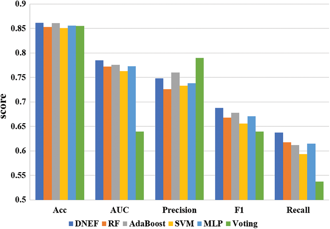
Figure 2: DNEF performance in the adult dataset

Fig. 3 demonstrates that DNEF and the baseline model performed on each metric on the REJAFADA dataset. DNEF achieved the best scores in the REJAFADA dataset, and the scores of Accuracy, AUC, and F1 indicators exceeded 0.98.

Figure 3: DNEF performance in the REJAFADA dataset

Fig. 4 shows the scores of DNEF and the baseline model on the IMDB dataset. In the IMDB high-dimensional sparse dataset, all ensemble models with the decision tree as base classifier performed worse than MLP and SVM. In this case, DNEF performed better than the three ensemble models of RF, AdaBoost, and Voting.

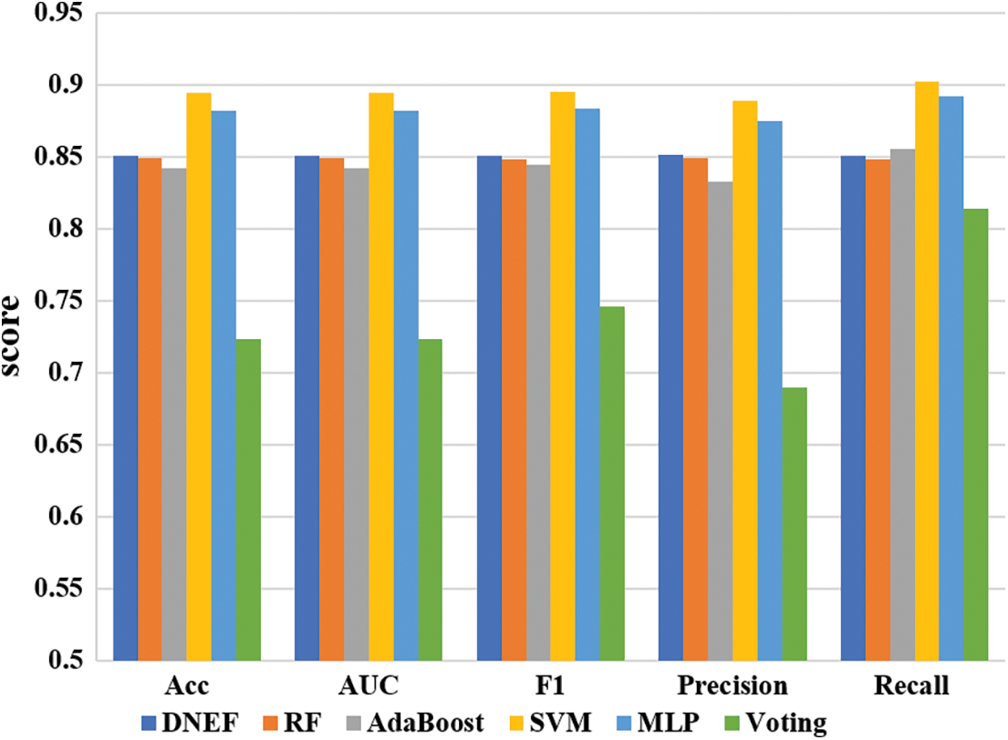
Figure 4: DNEF performance in the IMDB dataset

Fig. 5 illustrates the scores of DNEF and the baseline model for the Segmentation dataset. DNEF performed well in multi-class classification. DNEF outperformed RF, AdaBoost, SVM, and MLP in terms of Accuracy, F1 score, Precision, and Recall. Next, we will analyze in detail the specific performance of DNEF on each dataset.

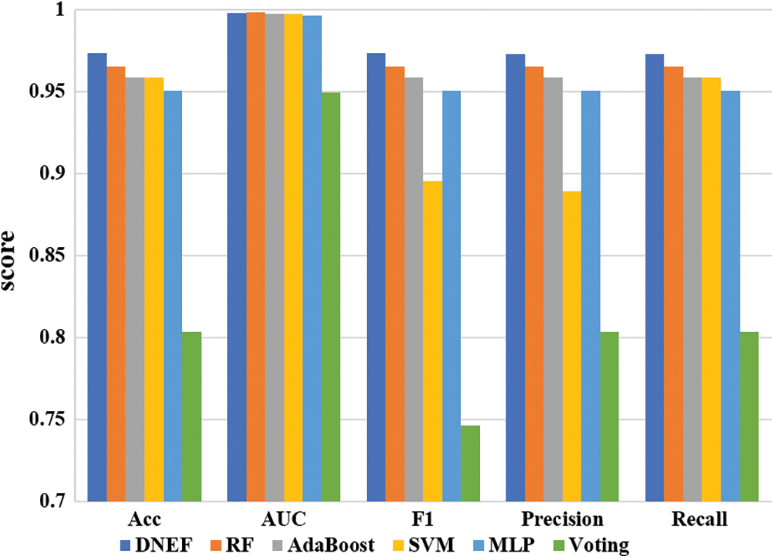
Figure 5: DNEF performance in the segment dataset

4.3.2 The Adult Dataset

Table 2 provides a detailed performance comparison of DNEF and other models. DNEF achieved first place with an accuracy rate of 86.18%, slightly higher than the second AdaBoost by 0.09%. Moreover, DNEF achieved the highest Recall among all models, with a 1.98% higher than RF. In terms of the F1 score, DNEF was 1.01% higher than the second-place AdaBoost. It can be seen from the AUC that DNEF was least affected by the number of positive and negative instances, which was 0.94% higher than AdaBoost. SVM and MLP were prone to overfitting on the Adult dataset with small feature dimensions; therefore, they were not as effective as DNEF. Voting (decision tree) had the worst ability to recognize negative instances, so the recall score was significantly lower than other models.

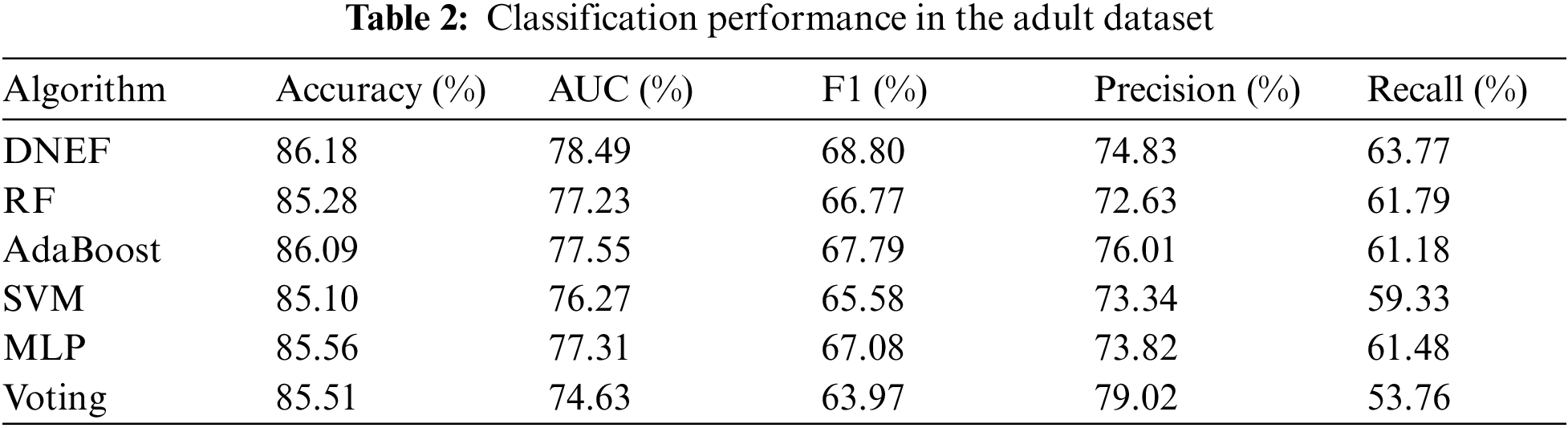
In the Adult dataset, the weighting strategy made DNEF more accurate than RF, SVM, and MLP. DNEF has achieved the highest recall score, possibly due to the transfer strategy that improves the recognition ability of positive instances and also favors the prediction of instances as positive classes, resulting in a decrease in Precision. DNEF not only surpassed AdaBoost in terms of accuracy but also led in F1 and AUC. We can conclude that the transfer strategy effectively enhanced DNEF’s ability to learn from data, making it an excellent classification framework.

4.3.3 The REJAFADA Dataset

Table 3 shows a detailed analysis of DNEF’s performance on the REJAFADA data. Compared to the other baseline models, DNEF achieved first place (98.09%) in experimental results in Accuracy, F1, and AUC. When all baselines achieved an accuracy of 98% or less, DNEF broke through to rank first with 98%, improving by 0.35% over the second-place RF and 0.65% over the third-place SVM. Although SVM has the highest Recall, its Precision was 2.55% lower than DNEF.

Since the baseline models had high accuracy rates of over 97%, the challenge of classification was concentrated in a small number of indistinguishable instances. DNEF effectively handled these tricky instances, benefiting from its transfer strategy. DNEF used the square root to scale down the weights of base classifiers with high accuracy, effectively solving the frequent overfitting problem. Among the three ensemble learning models, AdaBoost and Voting, DNEF outperformed them in terms of Accuracy, AUC, and F1 metrics. This superior performance was attributed to DNEF’s effective weighting strategy, which ensures accurate classification, and its transfer strategy, which enhances the recognition ability for samples from various classes. Consequently, DNEF exhibited exceptional performance in F1 and AUC. SVM and MLP had a significant bias in their ability to recognize positive and negative instances, leading to lower F1 scores.

4.3.4 The IMDB Dataset

In this subsection, we evaluated the performance of DNEF on the IMDB dataset based on Table 4 Regarding Accuracy, DNEF improved by 0.21% and 0.98% compared to RF and AdaBoost. The Precision of DNEF was slightly better than RF by 0.17%. Although the recall score of DNEF was 1.12% lower than that of AdaBoost, DENF scored higher than AdaBoost on all other metrics. In terms of F1 metrics, DNEF’s Precision and Recall combined exceed all ensemble models. Additionally, DNEF achieves the highest AUC score among all ensemble models, surpassing RF by 0.21%.

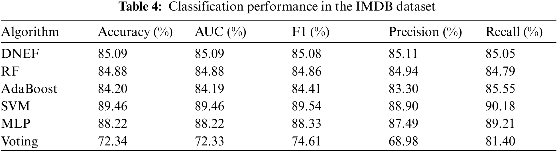
IMDB datasets were represented by tf-idf features with high-dimensional sparsity. According to Table 4, DNEF was still better than the ensemble learning models with decision trees such as RF, AdaBoost, and Voting in processing tf-idf feature data. The inferior performance of Voting suggested that the decision tree was inadequate for handling the IMDB dataset. Comparing the boosting ensemble strategy of AdaBoost with the bagging ensemble strategy of RF, we can obtain that DNEF surpasses these two representative ensemble models in terms of Accuracy, AUC, F1, and so on. SVM and MLP performed well on the IMDB dataset, which can be attributed to their ability to handle high-dimensional sparse data.

4.3.5 The Segmentation Dataset

In this subsection, we present an analysis of DNEF’s performance based on the results summarized in Table 5. Notably, DNEF demonstrated a significant advantage in multi-class classification. It achieved the highest Accuracy, F1, Precision, and Recall among the evaluated models. Specifically, in terms of Accuracy, DNEF surpassed the second-place RF by a margin of 0.97%, reaching 97.32%. Moreover, DNEF exhibited exceptional performance in F1, outperforming RF by 0.97%. Regarding Precision and Recall, DNEF consistently delivered the best results. The AUC of DNEF was only 0.04% lower than that of RF, underscoring its competitive performance across all measured metrics.

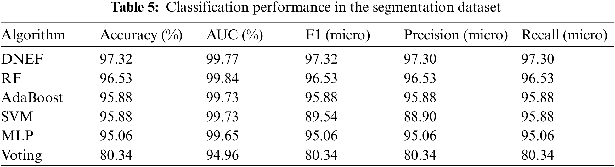
DNEF demonstrated strong performance in multi-class classification tasks, likely due to the effective utilization of its weighting strategy in conjunction with its transfer strategy. DNEF effectively addressed the complexity of multi-class classification through its weighting strategy. By adapting the classifier and instance weights for each class, DNEF further enhanced its accuracy. This tailored adjustment ensured that DNEF could effectively handle the intricacies associated with multi-class classification. Notably, DNEF maintained high classification accuracy while excelling in the F1 metric. This achievement was attributed to its transfer strategy, which intelligently guided indistinguishable instances from each class to the next hidden layer during operation. Consequently, DNEF maintained excellent Precision and Recall, further solidifying its suitability for multi-class classification tasks.

4.3.6 Parameter Analysis

The number of nodes in the hidden layer is an important parameter of DNEF. This subsection analyzes the impact of the number of nodes in the hidden layer on the performance of DNEF. The number of nodes in each hidden layer of DNEF was changed to observe the different effects during training. Fig. 6 displays the training loss of DNEF with three different numbers (1, 2, 3) of nodes per hidden layer on the Adult dataset. As the number of nodes in the hidden layer increased, the loss line became smoother, and the training loss decreased in Fig. 6. We analyzed the details of the three lines in Fig. 6 as follows:

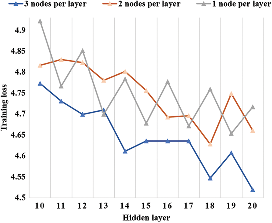
Figure 6: The training loss of DNEF with three different numbers of nodes

The gray line represents only one classifier in each layer of DNEF. In this case, the transfer strategy did not work. The training loss of the gray line decreased from 4.92 to 4.71. The loss decreased in an oscillating manner as the number of layers increased. Compared to the other lines, the gray line was the most oscillating and had a higher loss in the same number of hidden layer cases. The orange lines represented two nodes in each hidden layer in DNEF, in which case the transfer strategy worked. The training loss dropped from 4.81 to 4.66. Compared to the gray line, we could see that the orange line dropped more smoothly, and the loss was smaller with the same number of hidden layers. The blue line represents three nodes in each layer in DNEF. The blue line dropped from 4.77 to 4.51, which was the smallest of all the lines. From Fig. 6, the loss drop line was smoother than the other lines, and the training loss was consistently smaller. It showed that the weighting strategy worked better with the transfer strategy as the number of nodes in the hidden layer increased. This effectively reduced the training loss and made the training smoother.

4.4 Experiment Conclusion

We compare DNEF with the baseline algorithm on four datasets. Our experimental results demonstrate that DNEF outperforms the traditional ensemble model. DNEF significantly improved accuracy on the Adult, REJAFADA, and Segmentation datasets with F1 metrics compared to the baseline model. In the case of the high-dimensional dataset IMDB, DNEF outperforms traditional ensemble models in Accuracy, F1, AUC, and Precision. DNEF shows excellent performance, again proving its strength in multi-class classification. At the same time, we can infer the limitations of DNEF, as it is not directly comparable to MLP and SVM in high-dimensional data when using the decision tree as the base classifier. This is also the challenge of DNEF at present. It can be concluded from the parameter analysis that increasing the number of nodes benefits the effective implementation of DNEF’s transfer and weighting strategy, ultimately enhancing training effectiveness and stability.

DENF framework uses the weighting strategy between hidden layers and the transfer strategy in hidden layers, which is our main difference from other ensemble models. From the experimental results and parameter analysis, we conclude that it is the network structure of DNEF that contributes to its superior performance compared to other traditional ensemble models.

5  Conclusion

In this paper, we propose DNEF, a new ensemble learning architecture, DNEF incorporates a deep network structure that iterates between hidden layers and trains classifiers in parallel within the hidden layer. The weighting strategy trains the classifier based on the instance weights generated in the previous layer and further adjusts the instance weights; the transfer strategy operates within the hidden layer, selecting instances with weights for each node in the layer and combining them with the training data for the next layer. Compared to popular ensemble learning approaches, DNEF accounts for the relationship between base classifiers using the weighting strategy and enhances model complexity with the transfer strategy. The DNEF demonstrated promising results on four real datasets. Specifically, on the multi-class dataset Segmentation, DNEF achieved 0.9732 in Accuracy and F1, respectively. These experimental findings validate that DNEF, as a novel and exceptional deep ensemble architecture, outperforms traditional ensemble models. The primary contribution of this paper lies in exploring the ensemble structure under the network structure and expanding the ideas for ensemble learning. In our future work, we will extend DNEF in two ways: (1) We will explore various base classifiers for high-dimensional datasets. (2) We will also consider applying DNEF to different data such as images, sound signals, etc., and other learning tasks such as semi-supervised learning and incremental learning.

Acknowledgement: We thank the School of Mathematics and Information of South China Agricultural University for supporting this study.

Funding Statement: This work is supported by the National Natural Science Foundation of China under Grant 62002122, Guangzhou Municipal Science and Technology Bureau under Grant 202102080492, and Key Scientific and Technological Research and Department of Education of Guangdong Province under Grant 2019KTSCX014.

Author Contributions: Study conception and design: Ge Song; data processing: Changyu Liu, Zhuoyu Ou; analysis and interpretation of results: Ge Song, Yuqiao Deng, Siyu Yang; draft manuscript preparation: Siyu Yang, Ge Song. All authors reviewed the results and approved the final version of the manuscript.

Availability of Data and Materials: Four publicly datasets were used for analyzing our model. They can be found at https://archive.ics.uci.edu and https://ai.stanford.edu/~amaas/data/sentiment.

Conflicts of Interest: The authors declare that they have no conflicts of interest to report regarding the present study.

References

1. T. G. Dietterich, “Ensemble methods in machine learning,” International Workshop on Multiple Classifier Systems, vol. 1857, pp. 1–15, 2000. [Google Scholar]

2. M. P. Sesmero, J. A. Iglesias, E. Magán, A. Ledezma and A. Sanc, “Impact of the learners diversity and combination method on the generation of heterogeneous classifier ensembles,” Applied Soft Computing, vol. 111, pp. 107689, 2021. [Google Scholar]

3. L. Rokach, “Ensemble-based classifiers,” Artificial Intelligence Review, vol. 33, no. 1–2, pp. 1–39, 2010. [Google Scholar]

4. P. N. Thanh and M. Kappas, “Comparison of random forest, k-nearest neighbor, and support vector machine classifiers for land cover classification using sentinel-2 imagery,” Sensors, vol. 18, no. 2, pp. 18, 2017. [Google Scholar]

5. Q. Wang, Z. H. Luo, J. C. Huang, Y. H. Feng and Z. Liu, “A novel ensemble method for imbalanced data learning: Bagging of extrapolation-SMOTE SVM,” Computational Intelligence and Neuroscience, vol. 2017, pp. 1827016, 2017. [Google Scholar] [PubMed]

6. Y. Freund and R. E. Schapire, “Experiments with a new boosting algorithm,” in Proc. of ICML, San Francisco, CA, USA, pp. 148–156, 1996. [Google Scholar]

7. Y. Freund and R. E. Schapire, “A decision-theoretic generalization of on-line learning and an application to boosting,” Journal of Computer and System Sciences, vol. 55, no. 1, pp. 119–139, 1997. [Google Scholar]

8. Ambika and S. Biradar, “Survey on prediction of loan approval using machine learning techniques,” International Journal of Advanced Research in Science, Communication and Technology, pp. 449–454, 2021. [Google Scholar]

9. W. Wang, W. W. Guo, H. G. Liu, J. H. Yang and S. Y. Liu, “Multi-target ensemble learning based speech enhancement with temporal-spectral structured target,” Applied Acoustics, vol. 205, pp. 109268, 2023. [Google Scholar]

10. D. R. Nayak, R. Dash and B. Majhi, “Brain MR image classification using two-dimensional discrete wavelet transform and AdaBoost with random forests,” Neurocomputing, vol. 177, pp. 188–197, 2015. [Google Scholar]

11. J. M. M. de Lima and F. M. U. de Araujo, “Ensemble deep relevant learning framework for semi-supervised soft sensor modeling of industrial processes,” Neurocomputing, vol. 462, pp. 154–168, 2021. [Google Scholar]

12. B. H. Menze, B. M. Kelm, D. N. Splitthoff, U. Koethe and F. A. Hamprecht, “On oblique random forests,” Machine Learning and Knowledge Discovery in Databases, vol. 6912, pp. 453–469, 2011. [Google Scholar]

13. L. Zhang and P. N. Suganthan, “Random forests with ensemble of feature spaces,” Pattern Recognition, vol. 47, no. 10, pp. 3429–3437, 2014. [Google Scholar]

14. L. Zhang and P. N. Suganthan, “Oblique decision tree ensemble via multi-surface proximal support vector machine,” IEEE Transactions on Cybernetics, vol. 45, no. 10, pp. 2165–2176, 2015. [Google Scholar] [PubMed]

15. L. Zhang and P. N. Suganthan, “Benchmarking ensemble classifiers with novel co-trained kernal ridge regression and random vector functional link ensembles,” IEEE Computer International Magazine, vol. 12, no. 4, pp. 61–72, 2017. [Google Scholar]

16. L. V. Utkin, M. S. Kovalev and A. A. Meldo, “A deep forest classifier with weights of class probability distribution subsets,” Knowledge-Based Systems, vol. 173, pp. 15–27, 2019. [Google Scholar]

17. L. V. Utkin, M. S. Kovalev and F. P. Coolen, “Imprecise weighted extensions of random forests for classification and regression,” Applied Soft Computing, vol. 92, pp. 106324, 2020. [Google Scholar]

18. A. Paul, D. P. Mukherjee, P. Das, A. Gangopadhyay, A. R. Chintha et al., “Improved random forest for classification,” IEEE Transactions on Image Processing, vol. 27, no. 8, pp. 4012–4024, 2018. [Google Scholar] [PubMed]

19. P. A. A. Resende and A. C. Drummond, “A survey of random forest based methods for intrusion detection systems,” ACM Computing Surveys, vol. 51, no. 3, pp. 36, Article 48, 2018. [Google Scholar]

20. Y. Freund and R. E. Schapire, “A decision-theoretic generalization of on-line learning mand an application to boosting,” Journal of Computer and System Sciences, vol. 55, no. 1, pp. 119–139, 1997. [Google Scholar]

21. J. Chen, C. Yang, H. Q. Zhu, Y. G. Li and J. Gong, “Simultaneous determination of trace amounts of copper and cobalt in high concentration zinc solution using UV-vis spectrometry and Adaboost,” Optik, vol. 181, pp. 703–713, 2019. [Google Scholar]

22. B., Mücahid and R. Ceylan, “The effect of dictionary learning on weight update of AdaBoost and ECG classification,” Journal of King Saud University-Computer and Information Sciences, vol. 32, pp. 1149–1157, 2018. [Google Scholar]

23. L. Breiman, “Stacked regressions,” Machine Learning, vol. 24, no. 1, pp. 49–64, 1996. [Google Scholar]

24. D. H. Wolpert, “Stacked generalization,” Neural Networks, vol. 5, no. 2, pp. 241–259, 1992. [Google Scholar]

25. K. M. Ting and I. H. Witten, “Stacked generalization: When does it work,” in Proc. of IJCAI, Nagoya, JP, pp. 866–873, 1997. [Google Scholar]

26. M. Koopialipoor, P. G. Asteris, A. S. Mohammed, D. E. Alexakis, A. Mamou et al., “Introducing stacking machine learning approaches for the prediction of rock deformation,” Transportation Geotechnics, vol. 34, pp. 100756, 2022. [Google Scholar]

27. S. K. Kalagotla, S. V. Gangashetty and K. Giridhar, “A novel stacking technique for prediction of diabetes,” Computers in Biology and Medicine, vol. 135, pp. 104554, 2021. [Google Scholar] [PubMed]

28. A. M. P. Canuto, M. C. C. Abreu, L. M. Oliveira, J. C. Xavier Jr and A. M. Santos, “Investigating the influence of the choice of the ensemble members in accuracy and diversity of selection-based and fusion-based methods for ensembles,” Pattern Recognition Letters, vol. 28, no. 4, pp. 472–486, 2007. [Google Scholar]

29. V. C. Osamor and A. F. Okezie, “Enhancing the weighted voting ensemble algorithm for tuberculosis predictive diagnosis,” Scientific Reports, vol. 11, pp. 14806, 2021. [Google Scholar] [PubMed]

30. S. Y. Kim and A. Upneja, “Majority voting ensemble with a decision trees for business failure prediction during economic downturns,” Journal of Innovation & Knowledge, vol. 6, no. 2, pp. 112–123, 2021. [Google Scholar]

31. N. R. Sivakumar, S. M. Nagarajan, G. G. Devarajan, L. Pullagura and R. P. Mahapatra, “Enhancing network lifespan in wireless sensor networks using deep learning based graph neural network,” Physical Communication, vol. 59, pp. 1020716, 2023. [Google Scholar]

32. G. G. Devarajan, S. M. Nagarajan, S. I. Amanullah, S. S. A. Mary and A. K. Bashir, “AI-Assisted deep NLP-based approach for prediction of fake news from social media users,” IEEE Transactions on Computational Social Systems, pp. 1–11, 2023. [Google Scholar]

33. J. Escorcia-Gutierrez, R. F. Mansour, K. Beleño, J. Jiménez-Cabas, M. Pérez et al., “Automated deep learning empowered breast cancer diagnosis using biomedical mammogram images,” Computers, Materials & Continua, vol. 71, no. 3, pp. 4221–4235, 2022. [Google Scholar]

34. M. Ragab, A. Albukhari, J. Alyami and R. F. Mansour, “Ensemble deep-learning-enabled clinical decision support system for breast cancer diagnosis and classification on ultrasound images,” Biology, vol. 11, no. 3, pp. 439, 2022. [Google Scholar] [PubMed]

35. Z. H. Zhou and J. Feng, “Deep forest: Towards an alternative to deep neural networks,” in Proc. of IJCAI, Melbourne, Australia, pp. 3553–3559, 2017. [Google Scholar]

36. L. V. Utkin and M. A. Ryabinin, “A siamese deep forest,” Knowledge-Based Systems, vol. 139, pp. 13–22, 2018. [Google Scholar]

37. L. V. Utkin, “An imprecise deep forest for classification,” Expert Systems with Applications, vol. 141, pp. 112978, 2020. [Google Scholar]

38. C. Ma, Z. B. Liu, Z. G. Cao, W. Song, J. Zhang et al., “Cost-sensitive deep forest for price prediction,” Pattern Recognition, vol. 107, pp. 107499, 2020. [Google Scholar]

39. T. C. Zhou, X. B. Sun, X. Xia, B. Li and X. Chen, “Improving defect prediction with deep forest,” Information and Software Technology, vol. 114, pp. 204–216, 2019. [Google Scholar]

40. B. Yu, C. Chen, X. L. Wang, Z. M. Yu, A. Ma et al., “Prediction of protein-protein interactions based on elastic net and deep forest,” Expert Systems with Applications, vol. 176, pp. 114876, 2021. [Google Scholar]

41. R. Su, X. Y. Liu, L. Y. Wei and Q. Zou, “Deep-Resp-Forest: A deep forest model to predict anti-cancer drug response,” Methods, vol. 166, pp. 91–102, 2019. [Google Scholar] [PubMed]

42. H. Allende-Cid, R. Salas, H. Allende and R. Ñanculef, “Robust alternating AdaBoost,” in Pattern Recognition, Image Analysis and Applications, pp. 427–436, 2007. [Google Scholar]