Bearing Fault Diagnosis with DDCNN Based on Intelligent Feature Fusion Strategy in Strong Noise

1  Introduction

With the rapid improvement of science and technology and the development of modern industry, mechanical equipment is used in almost all daily production and life. Machinery tends to operate in complex environments, which makes modern intelligent sensing and maintenance very difficult. Although the speed and load equivalent can be artificially adjusted to keep the equipment in relatively stable operating conditions. However, some unavoidable factors such as mechanical vibration, speed fluctuation during operation, foreign body intrusion such as dust, insufficient lubrication, etc., will cause the detected signal to contain a large amount of noise. Therefore, the intelligent fault diagnosis of bearings must accurately extract important fault characteristic information from high-noise signals to determine the location and category of faults.

To enable the diagnosis of rolling bearing faults in complex environments, many methods have been proposed and implemented to eliminate the effects of noise. These methods can be broadly classified into two categories. One type removes noise from the signal by data pre-processing. One category directly extracts features from the highly noisy signal using deep learning models.

It is common to use signal processing methods to remove noise. Li et al. [1] used spectrum fusion to reconstruct the signal spectrum, which effectively reduces the noise interference in the resonant band. Chegini et al. [2] proposed an empirical wavelet transform (EWT) based technique for vibration signal denoising and bearing fault identification. Zheng et al. [3] proposed a denoising model for the sparsity characteristics of bearing fault signals in the frequency domain. Li et al. [4] and Ge et al. [5] decomposed bearing vibration signals to denoise and extract signal features by improving ensemble empirical mode decomposition (EEMD). These denoising methods of utilizing signal processing inevitably involve a great deal of expertise and experience, which leads to widely varying results in the processing of data depending on the skills of experts.

The deep learning model overcomes the aforementioned drawbacks. It can automatically extract data features and process complex data. Zhuang et al. [6] performed real-time bearing fault diagnosis by a clever combination of dilated convolution, long short-term memory network (LSTM) input gate structure, and residual network. Yan et al. [7] constructed an optimized stacked variational denoising autoencoder (OSVDAE) for the reliable fault diagnosis of bearings. Zou et al. [8] designed an adversarial denoising convolutional neural network (ADCNN) by combining GAN and CNN. Wang et al. [9] proposed a novel attention-guided joint learning convolutional neural network (JL-CNN) for mechanical equipment condition monitoring. Su et al. [10] built deep convolutional neural networks by stacking small convolutional kernels as the basic building blocks. To extract features from high-noise signals, different network combinations or superposition deepening models are used. This inevitably makes the structure of the model more complex. In addition, the input signals in the above research are all from a single sensor. If there is a large amount of noise in the input signal, the detection accuracy will be greatly reduced.

In fact, CNN has a satisfactory ability to capture and extract the rich features of the original fault signal. Excellent results can be achieved by using only a few layers of CNN. This paper employs a multi-sensor signal fusion strategy and leverages the remarkable capabilities of CNN to effectively capture and extract valuable features from original fault signals. It proposes a novel parallel multi-channel CNN architecture model. Xue et al. [11] proposed that the parallel multi-channel structure of 1D-CNN and 2D-CNN could deeply extract features. Ozcan et al. [12] implemented and tested a new bearing fault diagnosis system based on multi-channel 1D-CNN architecture that simultaneously utilizes multi-channel sensor data. They all prove that the multi-channel structure can further enhance the feature extraction ability of the model. However, the above multi-channel architecture only uses the parallel computing power of computers to repeatedly extract features from the same signal for fusion. The structure of multiple channels is uniform, complicated, and redundant. At the same time, there is no clear signal fusion strategy for the features extracted from multiple channels. The simple repetitive channel structure inevitably leads to single and redundant channels and is not suitable for bearing fault diagnosis in high-noise environments.

To reduce the effects of excessive noise, it is recommended to avoid relying solely on signals from a single sensor. To improve accuracy, it is advisable to consider data from multiple sensors. The absolute judgment of a single signal is avoided by comparing signals from different sensors. This reduces the error caused by noise, improving fault diagnosis performance. Different sensor signals are input through multiple channels. In the present multi-channel structure model, all channel configurations maintain high levels of consistency to ensure that the extracted features from each channel have the same dimensions and can be readily fused with each other. The recurrent channel structure involves extracting features from the input multiple times, with limited added benefits. To support the notion of multi-sensor joint diagnosis, a novel efficient signal fusion strategy is presented alongside a nov dual-channel structure.

The main idea of the parallel dual-channel model proposed in this paper is to integrate the detailed and deep features of the primary sensor signal with the global information and shallow features of the secondary sensor signal. The feature of the primary sensor signal is extracted by the small convolution kernel, which is used to judge the fault signal. The feature of the secondary sensor signal is extracted by the large convolution kernel to complement the defect feature. The problem of poor signal quality obtained from a single sensor in a high-noise environment is avoided. At the same time, a large convolution kernel is used to replace a multi-layer small convolution kernel in a channel to obtain a larger receptive field, reduce the training parameters of the model, and avoid the redundancy of channels.

The innovative contributions of this paper are as follows:

1.    The novel dual-channel convolution model for bearing diagnosis under complex working conditions is proposed. The redundant dual-channel structure is optimized, and excellent denoising performance and fault diagnosis are obtained.

2.    A new feature fusion method to improve the noise robustness of fault diagnosis models is discussed. Not only the number of parameters in training is greatly reduced, but also the stability performance of the model is enhanced.

3.    The superiority of the novel dual-channel convolution model was demonstrated through a multifaceted comparison of the dataset of Paderborn and Case Western Reserve University. The validity and accuracy of the model are ensured in strong noise environments.

The remainder of the paper is organized as follows: Section 2 details the proposed feature fusion strategy and the novel dual-channel model framework. Section 3 compares the performance of the proposed model and provides a visual analysis. Section 4 further verifies the model with additional datasets. Section 5 summarizes the work of this paper and looks forward to future research plans.

2  Feature Fusion Strategy and Proposed Framework

2.1 Proposed Feature Fusion Strategy

The general idea of the proposed feature fusion strategy is shown in Fig. 1. The detailed features of the primary signal are gradually extracted by using deep small convolution as the main basis for fault identification. To avoid the influence of high noise, shallow large convolution is used to quickly extract the global information of secondary signals as a complement to the defect features. The multi-sensor signals are fused at the feature level, and the features of the deep layer and shallow layer are taken into account to ensure the accuracy and stability of fault diagnosis. Finally, fault diagnosis is performed according to the fused feature information to classify the type and determine the cause of bearing failure.

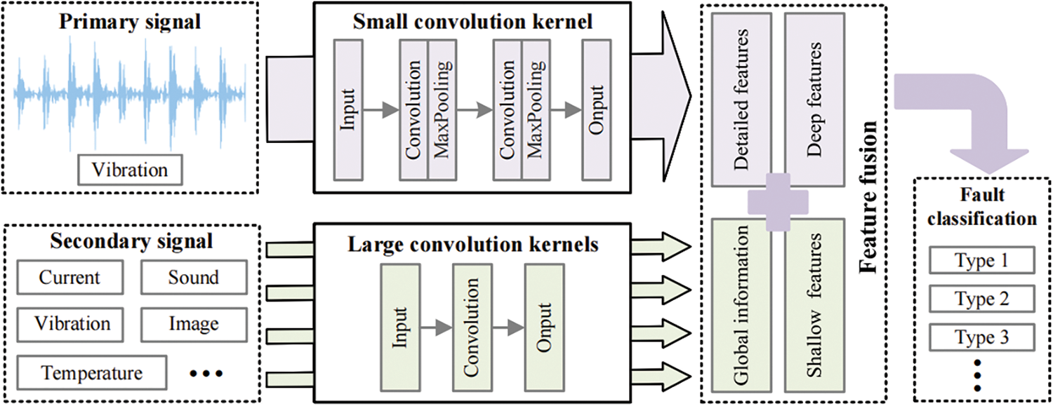
Figure 1: Feature fusion strategy diagram

The proposed feature fusion strategy considers different types of signal features, including four parts: detailed features, deep features, global information, and shallow features. Meanwhile, to enrich the diversity of extracted features, four types of features are extracted from two signals each. Detailed features and deep features come from primary signals, while global information and shallow features come from secondary signals. Bearing vibration is very sensitive to bearing damage, such as spalling, indentation, rust, cracking, wear, etc., which will be reflected in bearing and vibration measurements. Therefore, the vibration signal is used as the primary signal input. The selection of secondary signals is relatively wide. They can be current, sound, images, temperature, or even vibration signals from other places. The signal that can reflect the bearing change can be used as the secondary signal input. The fused signal features can carry more information and are not susceptible to noise interference. It can ensure the stability and robustness of the model in a complex environment.

2.2 Novel Dual-Channel Network Model

2.2.1 Construction of Dual-Channel Model

The proposed dual-channel network model is a 2D convolutional model that uses data from different sensors as input. The main channel uses a multi-layer small convolution kernel to extract the detailed features of the primary signal, while the supplementary channel uses a large convolution kernel to optimize the model, avoid the redundancy of the channel, and extract the global information of the secondary signal. After fusing the characteristic information of all channels, the output is finally classified by the full connection layer. The establishment process of the dual-input dual-channel convolutional neural network (DDCNN) model is shown in Fig. 2.

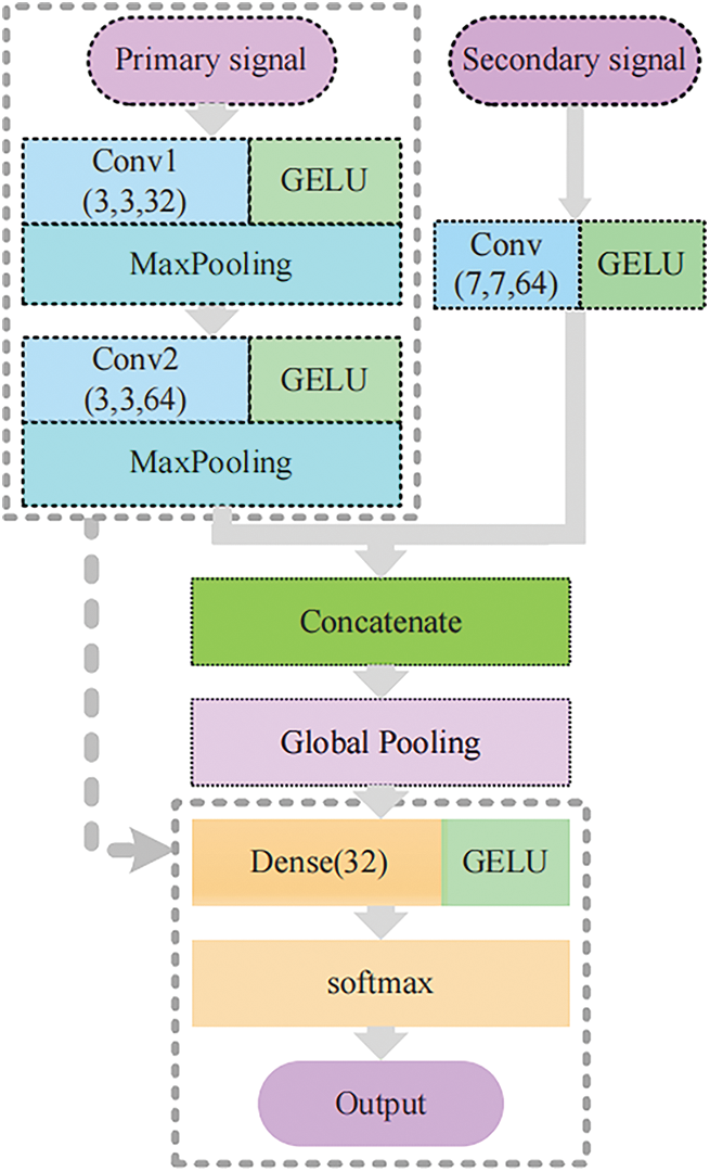
Figure 2: Establishment process of the dual-channel structure

Due to the uncontrollable influence of mixed dust, insufficient lubrication, mechanical resonance, and so on, the bearing will inevitably be doped with a lot of noise in operation. The first thing to consider is how to improve the performance of the model under heavy noise. The signal measured by the vibration sensor is the primary signal. However, the original one-dimensional vibration signal makes it difficult to achieve the ideal recognition effect due to the high noise. Given the stronger feature extraction ability of two-dimensional convolution, the model input is converted from the original one-dimensional vibration data to two-dimensional data. Then, multilayer convolution is used to extract the features of the signal step by step. To make the signal features more detailed, the small convolution kernel is used to focus the local features. The final main channel structure is shown in the dotted box in Fig. 2.

Under stable conditions, the model has a good performance. However, the vibration signal becomes significantly degraded due to the presence of high levels of noise pollution, resulting in a decrease in diagnostic accuracy. Therefore, the secondary sensor signals are added to further verify the discriminant results as a powerful supplement to the primary sensor signal. To avoid interfering with the primary sensor’s feature extraction, other secondary signals are input on separate channels. Simply repeating the original feature extraction module will inevitably lead to channel redundancy. Therefore, only one large convolutional layer is used to extract the signal features on the supplementary channel. By using one large convolutional layer instead of several small convolutional layers, the number of training parameters is greatly reduced. More importantly, it adds the shallow features and global information that is missing in the main channel. Before classification, the features extracted from the supplementary channel and the main channel are integrated to perform the final fault diagnosis.

2.2.2 Model Details

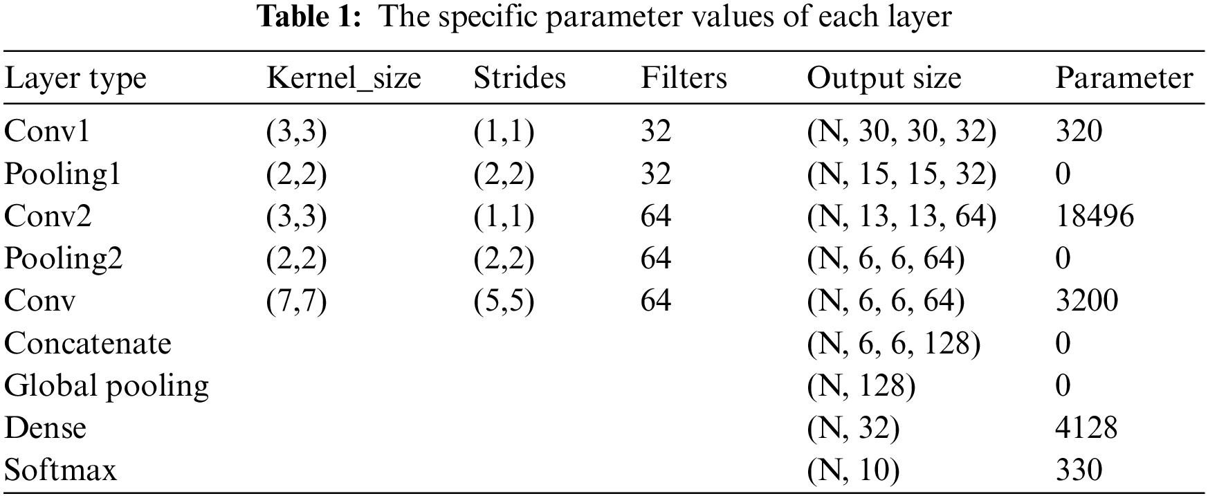
Based on the above ideas, we built the DDCNN model. The proposed DDCNN is a dual-channel 2D model with inputs from multiple sensors. The structure of the DDCNN model is shown in Fig. 3. Input1 which uses two convolutional-pool layers is the primary sensor data, and the detailed features are extracted using a 3 × 3 small convolution kernel with a step size of 1. Input2 which uses only one convolution layer is the secondary sensor data, and the global information is obtained using a 7 × 7 large convolution kernel with a step size of 5. After fusing the convolved dual-channel data, different bearing states are output using SoftMax classification through a global average pooling layer and a fully connected layer. The specific parameter values of each layer are shown in Table 1.

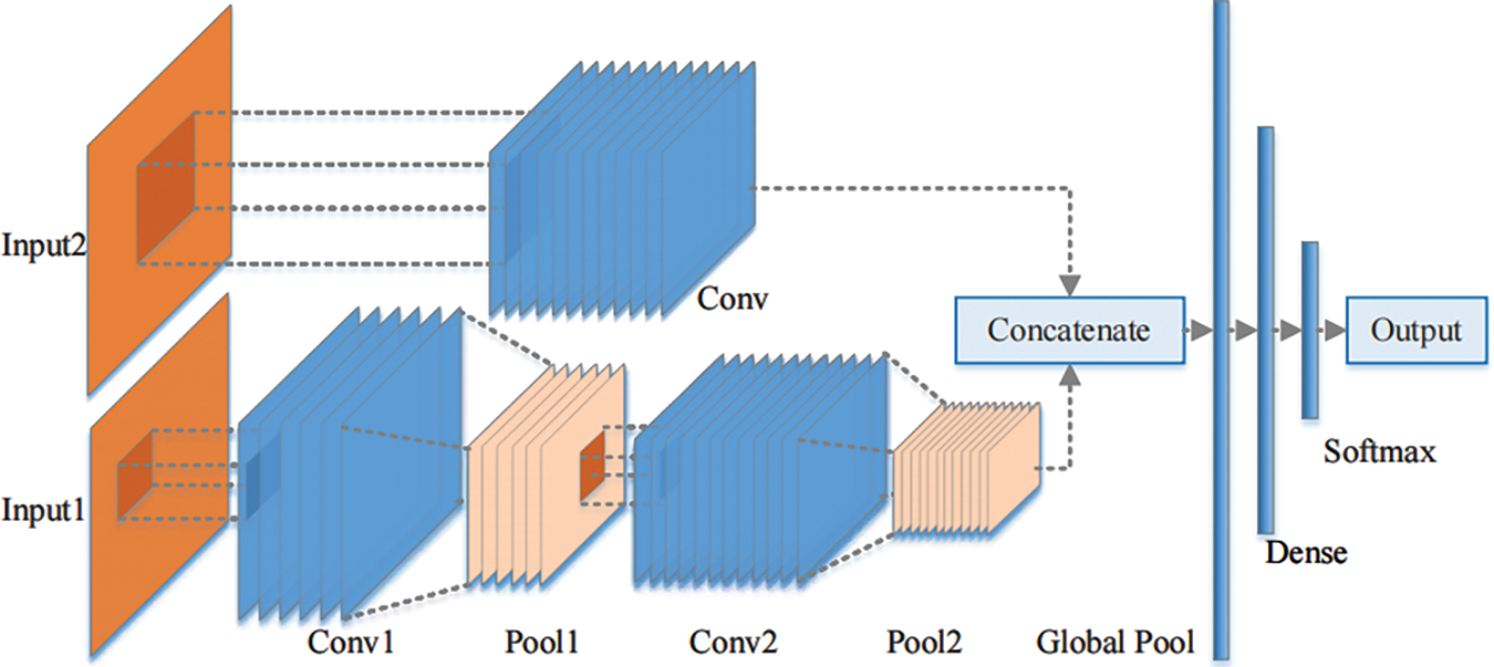
Figure 3: Architecture of the DDCNN model

3 × 3 is the smallest size that can capture information from eight neighborhoods of a pixel. Stacking two layers of small convolutional kernels ensures that detailed features of the defect information are extracted. At this point, the finite receptive field is equivalent to 5 × 5. Therefore, we use a large convolutional kernel of 7 × 7 with a step size of 5 in the other channel. The receptive field is expanded as much as possible without increasing parameters and running time. The larger the receptive field, the more global features are extracted and the better the recognition performance.

Gaussian Error Linear Unit (GELU) [13] is adopted as the activation function of the proposed model. GELU incorporates the idea of dropout in the activation, which mainly introduces randomness to the activation function and makes the model more robust in the training process. Compared to the commonly used RELU activation function, GELU does not lose characteristic information when the signal is less than 0. This allows the model to extract more detail from important sensor signals. It is given below:

GELU(x)=x∗Φ(x)≈0.5(1+tanh⁡[2π(x+0.044715x3)])(1)

where Φ(x) is cumulative distribution of the Gaussian normal distribution of x, and the final calculation results are approximate.

In order to obtain more accurate defect information and better identify defect categories, one_hot is used to label the data, categorical_crossentropy is used as the loss function, and Adam is used as the optimizer. In addition, it is worth noting that given the relatively slow gradient descent of the two-dimensional input, the learning rate takes on a function that decreases exponentially with the number of iterations. The dynamic learning rate ensures that the model can achieve the best performance in every stage of training. This is as follows:

αt=0.01∗0.96t(2)

The initial learning rate is 0.01 and t is the number of iterations. After 50 iterations, the learning rate is about 0.0013. The advantage is that it can get a higher descent rate at the beginning of the iteration and a better convergence with a smaller epoch. In the later stage of training, a small learning rate can ensure the stability of the model and avoid parameters oscillating between two sides of the optimal solution.

3  Model Comparative and Performance Test

The experimental data used in this section are from the rolling bearing database center of Case Western Reserve University (CWRU) in the United States. The CWRU data is one of the most commonly used data sets for bearing fault diagnosis [14], which sampling system is shown in Fig. 4. One acceleration sensor is placed above the bearing housing at the Fan End (FE), and one above Drive End (DE) of the motor to collect vibration acceleration signal of faulty bearing. The drive end-bearing fault data measured by sensors at different locations were obtained at a 12 kHz sampling frequency. The model performance test was conducted using FE data as the primary data and DE data as the secondary data.

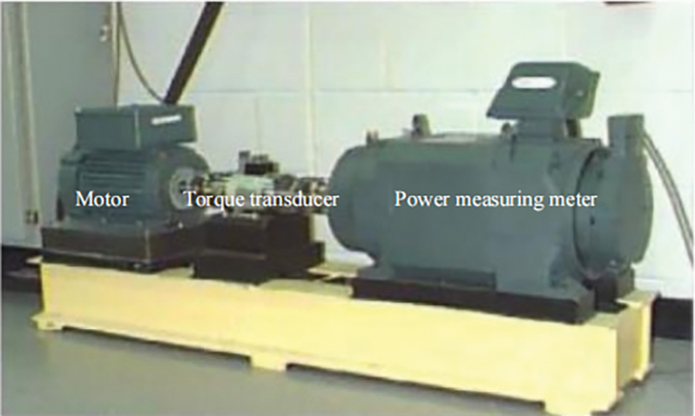
Figure 4: The CWRU bearing data sampling system

3.1 Data Processing Procedures

Considering the difference in data processing, the final performance of the model will be affected. Therefore, in order to obtain more accurate experimental results, the processing of data is clearly explained Fig. 5 illustrates the specific data processing procedure. On the left is a diagram of the data mixing. The data from all operating conditions are mixed in a certain proportion for training to adapt to a variety of conditions. Meanwhile, the amount of fault data at different locations is also reasonably distributed. The data pre-processing process is shown on the right. First, to cope with the complex practical application environment, raw data from various sensors are noise-enhanced. The data volume is then increased using data augmentation techniques. Finally, the data is reconstructed into a two-dimensional data input.

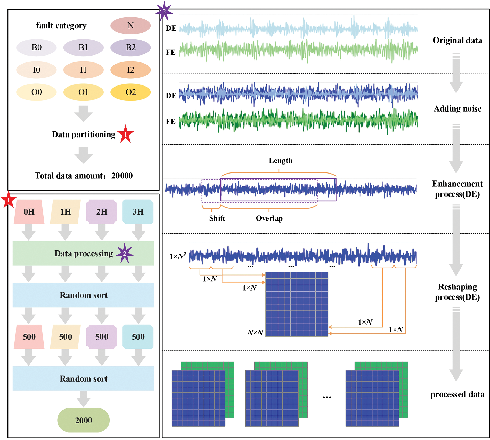
Figure 5: The specific procedures of data processing

The CWRU-bearing data is relatively simple and stable. Therefore, in this paper, random noise is added to the data in a way that simulates the noise signals that exist in practice. As noise increases, the signal becomes more blurred, and the corresponding features are more difficult to extract. Signal-to-Noise Ratio is used to measure the intensity of noise, which is expressed as:

SNR(dB)=10log10⁡(PSPN)(3)

where PS and PN represent the effective power of signal and noise respectively. In general, the stronger the noise entrained in the vibration signal, the smaller the SNR. When the SNR is 0, it means that the noise power is the same as the signal power. At this time, the signal reliability is extremely low, and the correct signal cannot be judged basically. As the noise continues to increase, SNR will be less than 0. This indicates that the noise power is greater than the signal power. It is very difficult to extract features from the signal due to the influence of a large amount of noise. When the noise exceeds a certain proportion, the collected signal will almost lose its function, and no useful characteristics can be obtained from it. To highlight the intense noise environment, the test was conducted with an SNR of −4.

For one-dimensional bearing fault vibration signals, data enhancement is usually performed by overlapping sampling with a sliding window. Suppose there is a window of sample length, and each time the sample interval is shifted by a certain amount. Then two sets of data obtained will have overlapping parts. This can be expressed as:

N=D−LS(4)

where N is the number of samples obtained, D is the length of the original data, L is the length of each training sample collected, and S is shift. To obtain more training data, the experiment uses an L value of 1024 and an s value of 128.

Two-dimensional image signals contain more in-depth and high-dimensional features compared to one-dimensional vibration time series signals, which are suitable for model generalization. Therefore, a one-dimensional original signal can be transformed into a two-dimensional signal as input in a superposition manner. First, every N point of the one-dimensional signal after maximum-minimum normalization is taken out as one of the rows of data in a two-dimensional signal; then the N rows of data are superimposed to form an N×N two-dimensional signal. The N value is 32 for the experiment.

Most of the diagnostic methods proposed so far are performed under the same operating conditions. In CWRU data, operating conditions refer to different workloads. However, the working load varies with the equipment products under complex running environments. Moreover, issues such as environmental noise and equipment aging can cause load to differ from the actual settings. As a result, traditional methods based on the same workload may not achieve original results in practical applications, and may even fail to identify faults [15].

In order to attenuate the impact of load as much as possible, the data from all different loads are mixed for training to extract features of fault data. With a certain amount of training data guaranteed, data are allocated by the structure: number of each type of load (500) * ten types of faults (10) * four types of loads (4). Total number of samples is 20,000. The ratio of training samples, validation samples, and test samples is 7:2:1, all of which are randomly selected without repetition from the samples after data enhancement, and the numbers are 14000, 4000, and 2000, respectively.

3.2 Noise-Resistant Test

In this paper, four CNN models with good performance and strong generality are used as comparison experiments. The WDCNN [16] is composed of five 1D convolution layers in alternating order with pooling layers. It mainly uses a wide kernel of the first convolutional layer to extract features and suppress high-frequency noise. The WKCNN [17] has a similar structure to the WDCNN, and the core idea is to widen the convolutional kernel and combine deep learning with other optimization algorithms. Both models are 1D-CNN networks. Wen et al. [18] proposed a New CNN based on LeNet-5, which has good potential in the field of fault diagnosis. AlexNet [19] is a classical network for processing images. The basic model is kept unchanged, and the size of the CNN layer and pooling layer is appropriately reduced so that it can handle small image data. Both models use two-dimensional image input. The DDCNN is a two-dimensional dual-input model proposed in this paper. In addition, we tested the model’s performance with only a single input, and the experimental results are denoted as DDCNN-. The DDCNN- and DDCNN models are identical. The difference is that the inputs of both channels of the DDCNN- are DE data.

A certain amount of noise is added to data for comparison experiments. The results with SNR of 0, −2, −4, −6, −8, and −10 dB are shown in Fig. 6. The accuracy of each model decreases significantly as the noise increases. The accuracy of 2D-CNN begins to exceed that of 1D-CNN. When the SNR is −4 dB, all models’ accuracy can still be maintained above 90%. And then accuracy starts to decrease rapidly with the increase of noise. Especially, 1D-CNN is seriously disturbed by noise. When the SNR reaches −10 dB, the WKCNN accuracy is 51.84%, and the WDCNN does not even exceed 50%, with only 46.52% accuracy. At this time, the New CNN accuracy is 78.85%, while the AlexNet effect is relatively poor, which can also reach 74.79%. It can be inferred that the two-dimensional model carries richer feature information and is less affected by noise interference than the one-dimensional model.

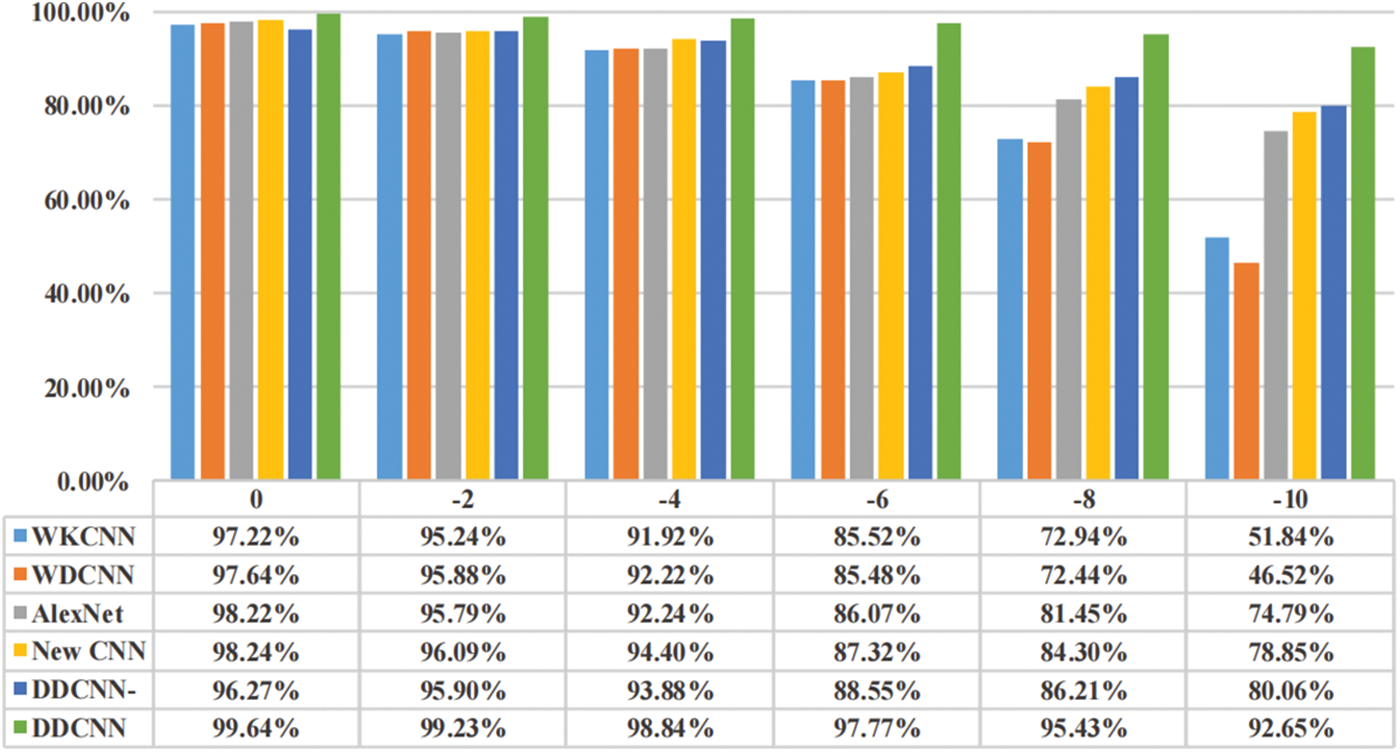
Figure 6: Comparison of the accuracy of each model under different SNRs

The proposed DDCNN model is much less affected by noise than other models. With a SNR of −4 dB, the accuracy is as high as 98.84%, and when the SNR reaches −10 dB, the accuracy is still 92.65%. Compared with other models, the recognition effect of DDCNN becomes more and more obvious with the increase in noise. It is well illustrated that the method of using FE and DE dual-data input for mutual verification can increase the noise-resistance interference ability of data, improve the robustness of the model, and ensure very high accuracy under the complex environment of strong noise. In addition, the DDCNN- model, which uses only DE as input, originally had slightly worse accuracy than other 2D models. However, after the SNR is less than −6 dB, the accuracy starts to significantly exceed the other models. This indicates that the dual-channel convolution has a strong anti-interference ability in a strong noise environment. The fusion of features extracted by dual-channel separately can enhance the feature extraction ability of the network and improve the stability and accuracy of the model.

3.3 Model Comparison

The accuracy of every model is above 90% when the SNR is −4 dB. Therefore, the specific training of each model at this time was examined. Accuracy curves and loss curves of the test are shown in Fig. 7.

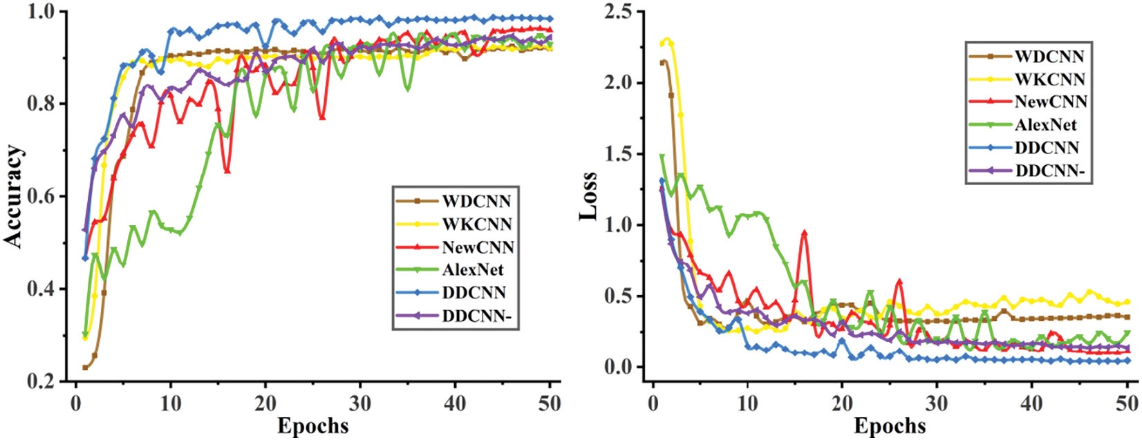
Figure 7: Variation curves when SNR is −4 dB

The accuracy and loss changes of WDCNN and WKCNN are generally similar. As a 1D-CNN model, the overall recognition effect is relatively stable and does not fluctuate much as the training of the network deepens. However, the accuracy is not as good as 2D-CNN under the strong noise environment. It is worth noting that loss functions of two 1D-CNN models tend to increase slightly after the epoch is greater than 10, and accuracy decreases slightly, showing signs of overfitting. New CNN and AlexNet, as 2D-CNN models, outperform 1D-CNN in accuracy when SNR is −4 dB. Although the fluctuations during the training process are relatively large, the overall trend is in line with expected results. And 2D-CNN can carry richer signal features by itself, so there is no overfitting within 50 epochs. Moreover, New CNN has a better recognition effect compared to AlexNet.

Due to the dual-channel mutual verification, DDCNN- has higher recognition accuracy, less overall fluctuation, and is more stable than other two-dimensional models. DDCNN with the addition of dual-data inputs further improves performance. It not only has a high feature extraction ability and recognition accuracy in a strong noise environment but also has excellent stability and robustness with no obvious fluctuation in verification results.

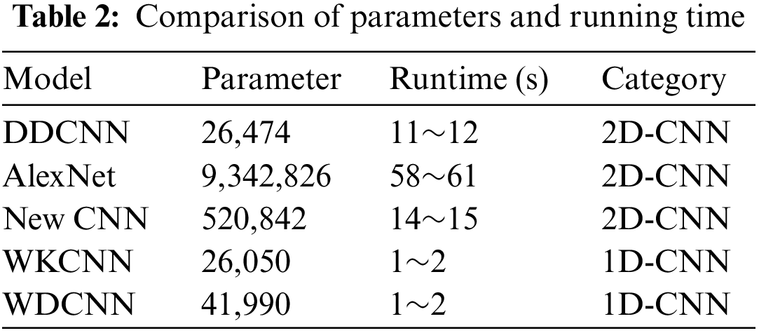
In addition, the number of parameters and the running time of an epoch for each model are recorded in Table 2. The proposed DDCNN model takes advantage of the optimized dual channel to avoid a large stacking of modules. The number of parameters and the running time are much smaller than other 2D-CNNs. Compared with 1D-CNN, the training speed is significantly slower, although the difference in the number of parameters is not large. This is the defect of the 2D model itself, which is difficult to enhance.

3.4 Workload Test

In order to avoid the situation that the accuracy of the model is greatly reduced by cross-loads, all workload data are mixed during data processing. So that the model can ignore the effects of load as much as possible and extract more fault characteristics. To verify the feasibility of this method, the trained models are tested separately with data from different loads. Fig. 8 exhibits the variation of model accuracy with load when SNR is −4 dB.

Figure 8: Variation of model accuracy with load when SNR is −4 dB

The accuracy of each model varies under different loads, but the absolute difference does not exceed 4%. Due to the fluctuation of model accuracy itself increases in a high noise environment, the overall results are still within an acceptable range. In addition, the average accuracy of the model under all loads remains highly consistent with experimental results in previous sections. It indicates that it is feasible to mix the data of different loads together for training.

The proposed DDCNN model has an accuracy difference of only 1.65% between loads. It is the smallest variation among all models. It shows that the DDCNN is better than other models in ignoring the differences brought by load and focusing on the characteristic information of the fault itself.

3.5 Inputs Comparison

Each of the bearing fault diagnosis datasets of Western Reserve University contains the fault data of DE and FE sensors that have not been fully utilized in other studies. An idea of feature fusion is proposed based on this, which focuses on detailed features of data measured by the key sensor and simply obtains global information of the other sensor for the supplement. The results of comparing different data as inputs are shown in Fig. 9, which proves the feasibility of this idea. The accuracy of “FE, FE” as input reaches 96.93%, which is 2.92% higher than the accuracy of “DE, DE” as input. This indicates that FE data is better overall and carries more information than DE data.

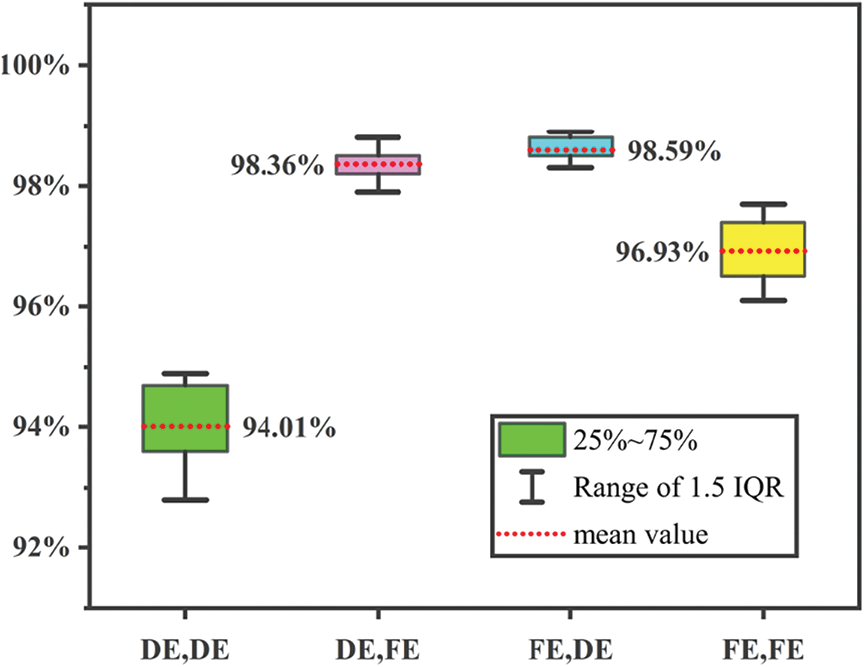
Figure 9: Comparison of different input results

The accuracy of using only DE data or FE data is not as good as using both. In addition, the results of both using DE and FE data as input have much less fluctuation, which obviously increases the stability of the model. In comparison, the best results can be obtained by processing FE data with the small convolutional kernel while processing DE data with the large, which also verifies that FE data has more advantages than DE data, and the features are relatively more obvious.

In summary, the proposed model uses dual data as input: the small convolutional kernels are used to extract detailed features of FE data, and the large convolutional kernel is used to obtain global information on DE. The model has a better recognition effect and higher accuracy compared with single data input, and the output results fluctuate less and have strong stability and robustness.

3.6 Visual Analysis

3.6.1 Confusion Matrix

Confusion matrix is a kind of visual method to evaluate the accuracy of classification models. The X-axis represents the prediction label and the Y-axis represents the real label. A confusion matrix usually fills the matrix with the number of categories. However, the data of the experiment in this paper is divided randomly, and each type of fault number is around 200, which is not the same. In order to make the visualization results more intuitive, the confusion matrices are normalized.

It shows the confusion matrix of the proposed model without noise in Fig. 10a. The classification accuracy basically reached a hundred percent at this time. Only in the case of the OR014 fault can it be classified as a B014 fault with a small probability. The confusion matrix when adding noise with an SNR of −4 is shown in Fig. 10b. It is obvious that fault classification errors are concentrated between the outer ring fault and the ball fault. Among them, OR014 and B007 faults and OR014 and B014 faults are mainly confused. The overall phenomenon is similar to the confusion matrix without adding noise.

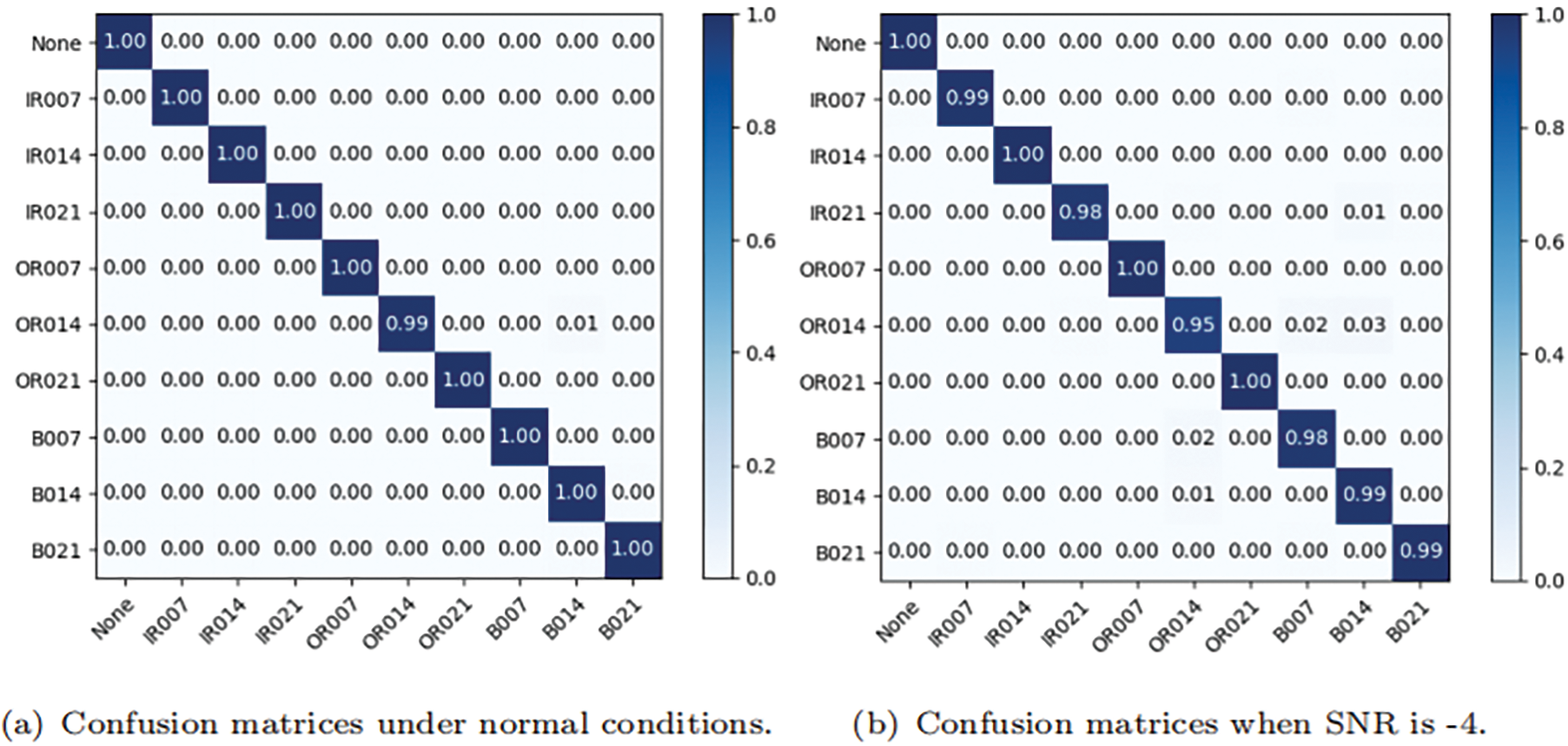
Figure 10: Classification results of the DDCNN

In general, The DDCNN model has high fault classification accuracy and good recognition ability even in strong noise environments. Moreover, fault classification errors are mainly between OR014 and B007 or B014, which can be improved to further enhance the performance of the DDCNN model.

3.6.2 T-SNE-Based Visualization

T-distributed Stochastic Neighbor Embedding (T-SNE) was proposed by Van der Maaten et al. in 2008 [20]. It is the most effective data dimension reduction and visualization method at present. The distributions of the 10 feature data are mapped onto a two-dimensional plane through T-SNE, and the classification visualization results of key layers are drawn in the DDCNN model when the SNR is −4, as shown in Fig. 11.

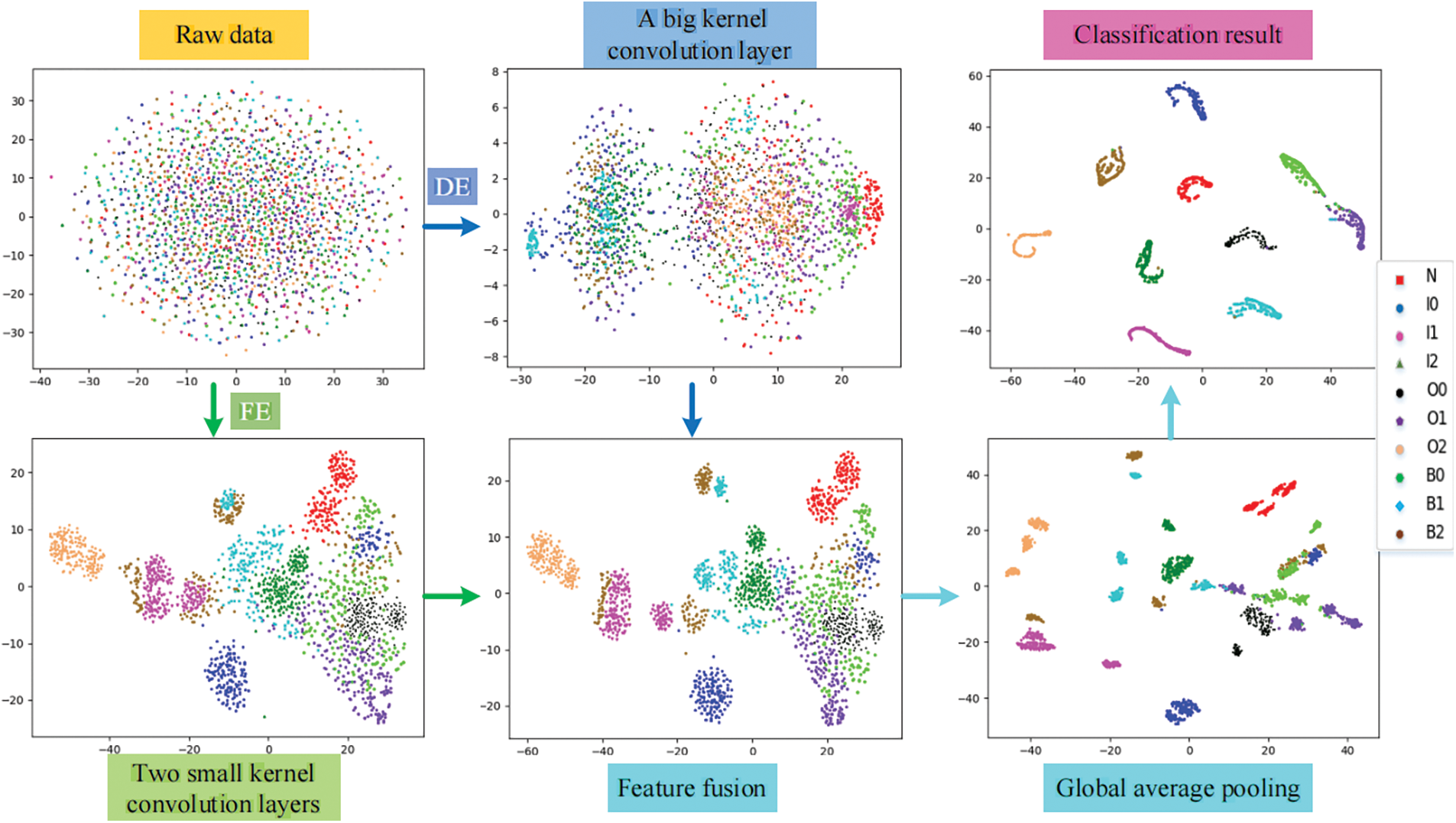
Figure 11: Feature visualization of the DDCNN model based on T-SNE

The original input is disorganized, with the highest degree of confusion. The data of DE go through a layer of large convolution, clustering for only part of the fault feature. After two layers of small convolution and pooling, the confusion degree of FE data is greatly reduced, but some faults still exist mixing phenomenon. The boundary of mixed fault signals is clearer after signal features of both ends are fused. In the global average pooling layer, signal features are basically clustered into small pieces with a certain degree of mixing. Finally, each fault feature is further aggregated and separated significantly between groups by classifying output through the full connection layer.

It can be inferred that the mixing degree between different features is small after the combined efforts of dual data and dual channels. Therefore, it has proved useful for the model to converge more easily and classify better. In addition, observing the final T-SNE visualization clustering results, it can be seen that the most confusion occurred when green (B007) and light blue (B014) were clustered into purple (OR014). This is consistent with the conclusion of the confusion matrix in the previous section.

4  Further Validation

The CWRU dataset consists of fault data collected under stable conditions with minimal operational noise, including speed, load, and other factors. In previous experiments, adding random noise to the dataset was used to simulate complex operating environments, resulting in relatively good experimental results. This section describes further experiments using the bearing dataset from the University of Paderborn in Germany. Fig. 12 is an illustration of the test platform. The data collected from it is more complex and can better represent the actual operating conditions.

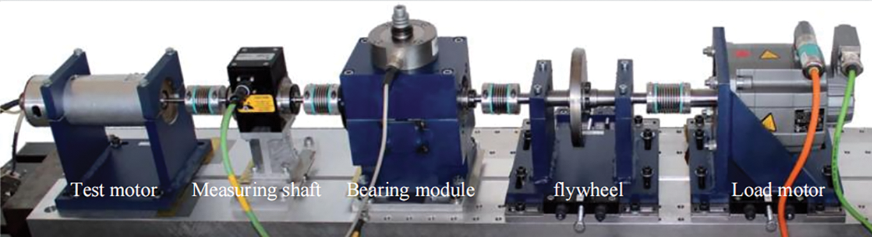
Figure 12: The Paderborn dataset test platform

The Paderborn Condition Monitoring (CM) dataset contains vibration and motor current signals. The vibration signal is used as the primary data, and the motor current signal as the secondary data for further validation.

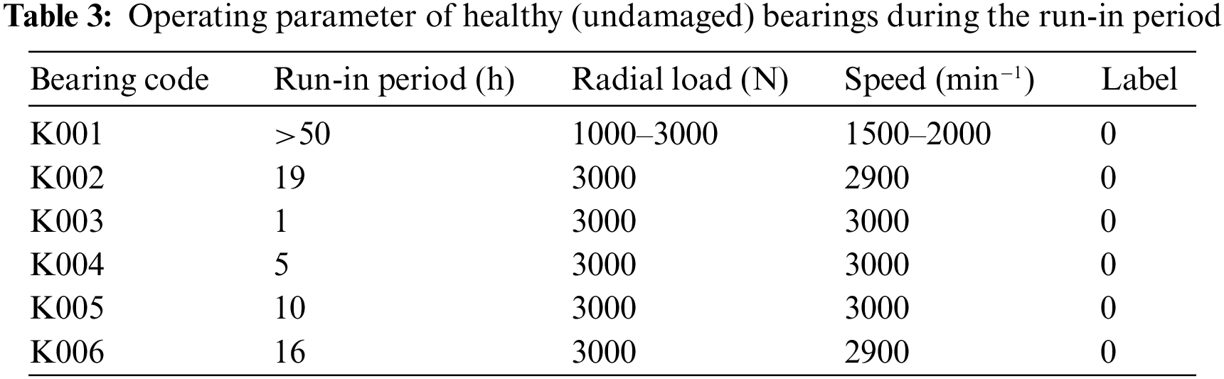
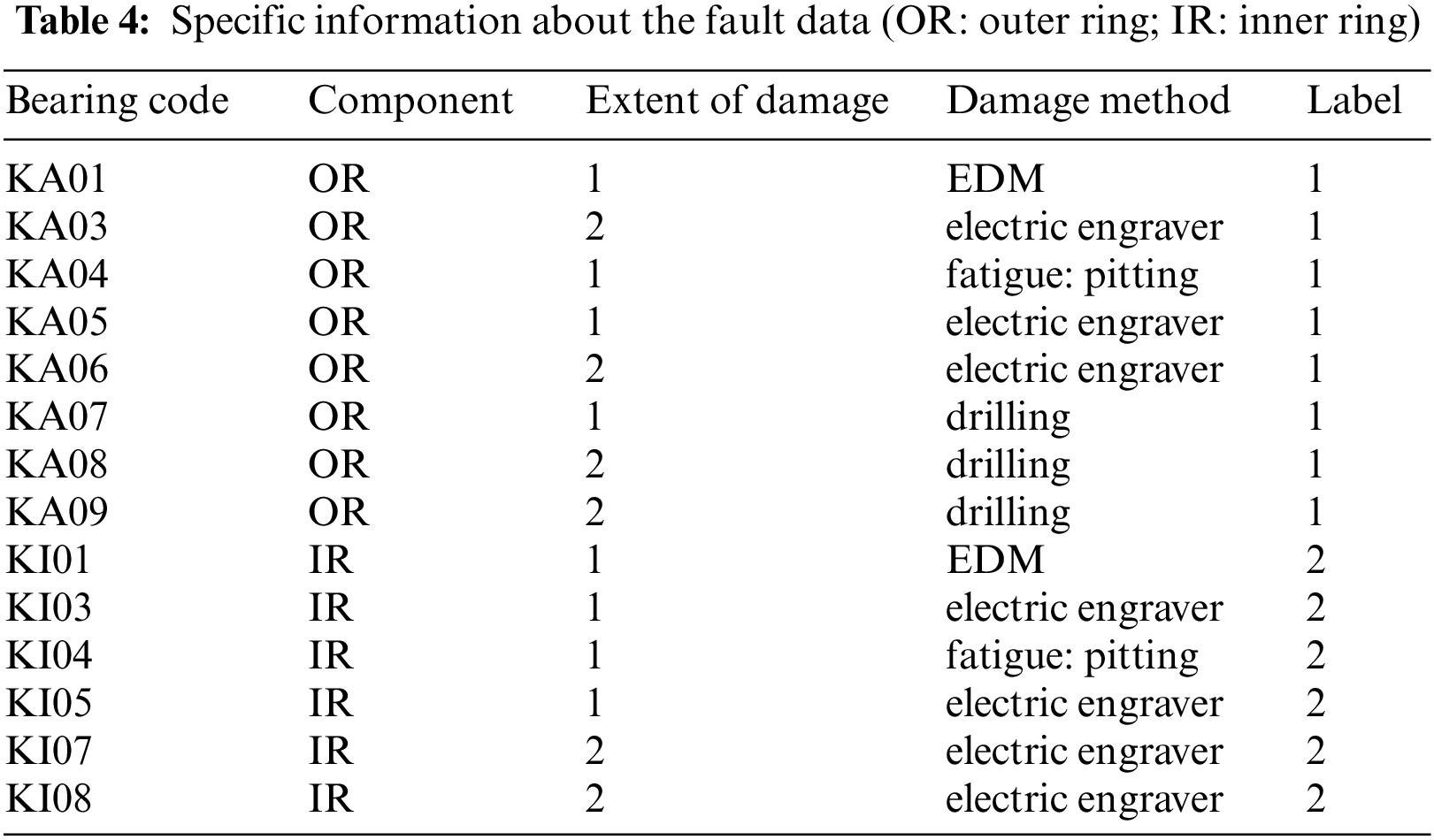
The data collected is more complex and representative of actual operating conditions, with key parameters such as speed, radial force and load torque artificially set during operation. In experiments, these parameters were varied to simulate different operating conditions. Uncontrollable factors such as run-in time, extent of damage, and damage method were treated as ambient noise. The focus was solely on damage location classification. Table 3 provides data for various normal categories, while Table 4 provides specific information on failure data. To increase the class balance and reflect real-world scenarios, the number of outer ring defects was slightly higher than other categories.

4.1 Noise Immunity Comparison

In this experiment, 250 data points were collected for each of the 20 different Bearing Codes, resulting in a total of 5000 data points per category of operating conditions. The data was then mixed together for all running conditions and only fault categories were classified. The data processing and model parameters remained unchanged from previous experiments.

Fig. 13 depicts the experimental results of the model on Paderborn data, which show that classification accuracy substantially decreases with the inclusion of a relatively large amount of useless information. The overall results remain consistent with previous experiments involving the addition of random noise to the data. Both 1D-CNN models perform significantly worse than the 2D-CNN model. The proposed DDCNN model achieves an accuracy of 91.85%, outperforming all other models by utilizing a dual data feature fusion approach and dual-channel input. Compared to other models, the DDCNN model exhibits a smaller overall error range and more stable experimental results.

Figure 13: Comparison of models

4.2 Operating Conditions Comparison

During model training, data from all running conditions were mixed together. Table 5 shows the four running conditions, with T4 as the baseline condition. Data for different running conditions were obtained by separately varying the speed, load, and radial force based on the T4 condition.

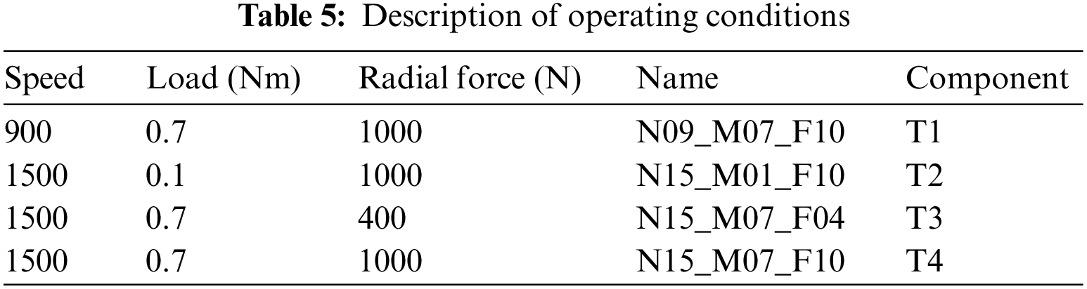
Fig. 14 depicts the results of testing the trained model under different running conditions, evaluated using the F1 score. The overall evaluation of the five models in the T4 running condition is consistent with previous results. However, as running conditions changed, the recognition accuracy showed some fluctuations. Reduction of load led to improved model performance while reduction of radial force resulted in worse performance. Nevertheless, the overall changes were insignificant and within acceptable limits. Changes in rotational speed had the greatest impact on model performance due to temporal compression or stretching of data, which reduced the amount of data collected per unit time. Despite using the same input data length of 1024, a change in rotational speed represented a completely different data segment, resulting in rapid degradation of model performance.

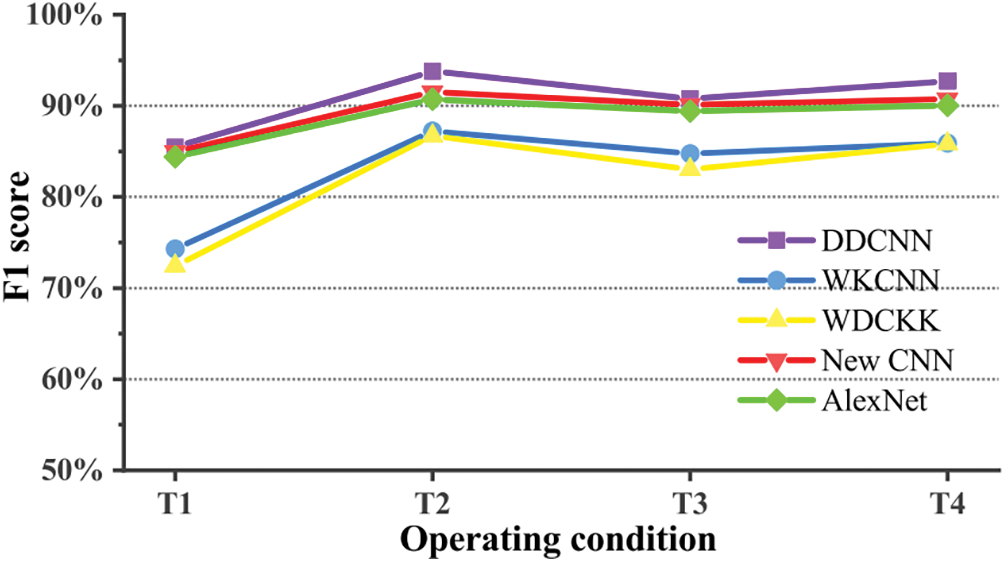
Figure 14: The results obtained by the model under different operating conditions

4.3 Inputs Comparison

Vibration and motor current signals are used in the Paderborn dataset. Experiments with different input channels show the advantages of the proposed multi-data feature fusion strategy. The experimental results are shown in Fig. 15. The darker the color, the higher the accuracy, and the larger the area, the more stable the results.

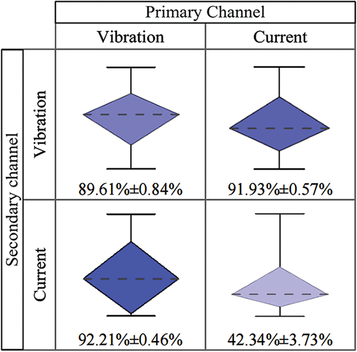
Figure 15: Multi-data fusion test

The detailed features of the vibration signal were extracted from the main channel, and the global features of the current signal were obtained from the supplementary channel. The best diagnostic results were obtained after the fusion of the two features. Not only the recognition accuracy is the highest, but also the fluctuation is the lowest, and the model is the most stable. It fits our strategy perfectly. In addition, when only the current signal is input, the diagnostic accuracy is less than 50%. If it is added as a secondary signal, it can greatly improve the diagnostic ability of the model. The results of the experiment with the current signal as the key signal and the vibration signal as the auxiliary signal are better than expected, even better than the results of the two channels with the vibration signal. The reason may be that the difference between the convolution layers of the two channels is not large enough. With one layer of large 7 × 7 convolution instead of two layers of small 3 × 3 convolution, the overall depth change is small. Of course, this also proves the superiority of multiple data input.

5  Conclusion

This paper proposes a primary and secondary fusion strategy for fault diagnosis using data obtained from different sensors. The DDCNN model is based on this method and optimizes the original two-channel structure to enhance feature extraction abilities. Experiments on two bearing fault datasets show that the model maintains high accuracy and recognition performance even in noisy environments. However, the proposed method only fuses two types of sensor data, and further investigation is required to verify the advantages of multi-data fusion for fault diagnosis. Additionally, the channel structure optimization is only suitable for inputs smaller than 64 × 64, and the model may fail for the larger two-dimensional inputs due to dimensional mismatch. Future work will optimize the channel structure to better adapt to inputs of varying dimensions.

Acknowledgement: The authors would like to thank the Shanxi Key Laboratory of Micro Nano Sensors & Artificial Intelligence Perception. Reviewers are also appreciated for their critical comments.

Funding Statement: This work was supported by the Key Research and Development Plan of Shanxi Province (Grant No. 202102030201012).

Author Contributions: The authors confirm contribution to the paper as follows: study conception and design: C. He, R. Hao; analysis and interpretation of results: K. Yang, Z. Yuan; draft manuscript preparation: C. He, R. Wang; review and editing: R. Hao, S. Sang. All authors reviewed the results and approved the final version of the manuscript.

Availability of Data and Materials: The experimental data used in this paper is from the rolling bearing database center of Case Western Reserve University (CWRU) in the United States (https://engineering.case.edu/bearingdatacenter, accessed on 02/11/2023) and the bearing dataset of the University of Paderborn, Germany (https://mb.uni-paderborn.de/en/kat/main-research/datacenter/bearing-datacenter, accessed on 02/11/2023).

Conflicts of Interest: The authors declare that they have no conflicts of interest to report regarding the present study.

References

1. Y. Li, G. Cheng and C. Liu, “Research on bearing fault diagnosis based on spectrum characteristics under strong noise interference,” Measurement, vol. 169, no. 1, pp. 108509, 2021. [Google Scholar]

2. S. N. Chegini, A. Bagheri and F. Najafi, “Application of a new EWT-based denoising technique in bearing fault diagnosis,” Measurement, vol. 144, no. 1, pp. 275–297, 2019. [Google Scholar]

3. K. Zheng, T. Li, Z. Su and B. Zhang, “Sparse elitist group lasso denoising in frequency domain for bearing fault diagnosis,” IEEE Transactions on Industrial Informatics, vol. 17, no. 7, pp. 4681–4691, 2020. [Google Scholar]

4. R. Li, C. Ran, B. Zhang, L. Han and S. Feng, “Rolling bearings fault diagnosis based on improved complete ensemble empirical mode decomposition with adaptive noise, nonlinear entropy, and ensemble svm,” Applied Sciences, vol. 10, no. 16, pp. 5542, 2020. [Google Scholar]

5. J. Ge, T. Niu, D. Xu, G. Yin and Y. Wang, “A rolling bearing fault diagnosis method based on EEMD-WSST signal reconstruction and multi-scale entropy,” Entropy, vol. 22, no. 3, pp. 290, 2020. [Google Scholar] [PubMed]

6. Z. Zhuang, H. Lv, J. Xu, Z. Huang and W. Qin, “A deep learning method for bearing fault diagnosis through stacked residual dilated convolutions,” Applied Sciences, vol. 9, no. 9, pp. 1823, 2019. [Google Scholar]

7. X. Yan, Y. Xu, D. She and W. Zhang, “Reliable fault diagnosis of bearings using an optimized stacked variational denoising auto-encoder,” Entropy, vol. 24, no. 1, pp. 36, 2021. [Google Scholar] [PubMed]

8. L. Zou, Y. Li and F. Xu, “An adversarial denoising convolutional neural network for fault diagnosis of rotating machinery under noisy environment and limited sample size case,” Neurocomputing, vol. 407, no. 1, pp. 105–120, 2020. [Google Scholar]

9. H. Wang, Z. Liu, D. Peng and Z. Cheng, “Attention-guided joint learning CNN with noise robustness for bearing fault diagnosis and vibration signal denoising,” ISA Transactions, vol. 128, no. 1, pp. 470–484, 2022. [Google Scholar] [PubMed]

10. K. Su, J. Liu and H. Xiong, “Hierarchical diagnosis of bearing faults using branch convolutional neural network considering noise interference and variable working conditions,” Knowledge-Based Systems, vol. 230, no. 1, pp. 107386, 2021. [Google Scholar]

11. F. Xue, W. Zhang, F. Xue, D. Li, S. Xie et al., “A novel intelligent fault diagnosis method of rolling bearing based on two-stream feature fusion convolutional neural network,” Measurement, vol. 176, no. 1, pp. 109226, 2021. [Google Scholar]

12. I. H. Ozcan, O. C. Deveciogu, T. Ince, L. Eren and M. Askar, “Enhanced bearing fault detection using multichannel, multilevel 1D CNN classifier,” Electrical Engineering, vol. 104, no. 2, pp. 435–447, 2022. [Google Scholar]

13. D. Hendrycks and K. Gimpel, Gaussian error linear units (GELUs), 2016. [Online]. Available: https://doi.org/10.48550/arXiv.1606.08415 (accessed on 25/10/2023) [Google Scholar] [CrossRef]

14. Y. Yoo, H. Jo and S. W. Ban, “Lite and efficient deep learning model for bearing fault diagnosis using the CWRU dataset,” Sensors, vol. 23, no. 6, pp. 3157, 2023. [Google Scholar] [PubMed]

15. Y. Gao, L. Gao, X. Li and Y. Zheng, “A zero-shot learning method for fault diagnosis under unknown working loads,” Journal of Intelligent Manufacturing, vol. 31, no. 4, pp. 899–909, 2020. [Google Scholar]

16. W. Zhang, G. Peng, C. Li, Y. Chen and Z. Zhang, “A new deep learning model for fault diagnosis with good anti-noise and domain adaptation ability on raw vibration signals,” Sensors, vol. 17, no. 1, pp. 524, 2017. [Google Scholar]

17. X. Song, Y. Cong, Y. Song, Y. Chen and P. Liang, “A bearing fault diagnosis model based on CNN with wide convolution kernels,” Journal of Ambient Intelligence and Humanized Computing, vol. 13, no. 1, pp. 4041–4056, 2022. [Google Scholar]

18. L. Wen, X. Li, L. Gao and Y. Zhang, “A new convolutional neural network-based data-driven fault diagnosis method,” IEEE Transactions on Industrial Electronics, vol. 65, no. 1, pp. 5990–5998, 2017. [Google Scholar]

19. F. N. Iandola, S. Han, M. W. Moskewicz, K. Ashraf, W. J. Dally et al., SqueezeNet: AlexNet-level accuracy with 50x fewer parameters and <0.5 MB model size, arXiv preprint, 2016. [Online]. Available: https://doi.org/10.48550/arXiv.1602.07360 (accessed on 25/10/2023) [Google Scholar] [CrossRef]

20. L. Van der Maaten and G. Hinton, “Visualizing data using t-sne,” Journal of Machine Learning Research, vol. 9, no. 1, pp. 2579–2605, 2008. [Google Scholar]