Research on Interpolation Method for Missing Electricity Consumption Data

1  Introduction

In the operation of the power grid, the difference between the power supply and sold counted by the measuring meter is called the statistical power line loss, and the corresponding power line loss rate is termed the statistical line loss rate [1]. Power supply enterprises hope that through the calculation and analysis of power line loss, they can dynamically and accurately propose loss reduction targets for power line objects. Inaccurate user metering circuits, such as abnormal behavior of electricity consumption and inaccurate magnification of metering devices, are important reasons for the fluctuation of the power line loss rate [2–5]. In the intelligent analysis and modeling of abnormal power consumption, there are evaluation indicators like power, load, alarm, and line loss. The data quality of these indicators directly affects the result accuracy and the evaluation standard of the models. Consequently, the data interpolation of missing values poses foundational importance to data analysis in diverse fields.

To achieve better modeling and analysis effects, the sample data needs to be preprocessed firstly, such as the missing data of power line loss needs to be filled by the results of appropriate algorithms, and then the power line loss rate can be calculated by using the topological relationship of the power line loss of branch lines. According to statistics, 0.5% of data missing is equal to the situation that 5% noise is injected into the analyzed dataset [6,7]. This is why in many scientific disciplines; data interpolation is a frequently-used method to complete missing data or to increase its resolution [8–11]. Thus, missing data recovery has also become a research hotspot in a wide range of fields. The idea of missing data interpolation with possible values comes from the fact that interpolating missing data with the most probable values produces less information loss than deleting incomplete samples altogether. Many different methods have been developed to implement missing data interpolation depending upon the nature of the data and the accuracy required. The main methods are based on statistical missing data interpolation methods [12–14] and machine learning (ML) based classification methods [15–19]. By assuming the normal distribution of the dataset, Junger et al. [12] proposed an EM algorithm-based method to implement the imputation of missing data in time series for air pollutants. Despite obtaining good accuracy and precision, their proposed imputation method is strictly subject tothe assumption conditions. Based on the random forest (RF) algorithm, Stekhoven et al. [20] introduced a iterative imputation method, which they termed missForest, for the task of mixed-type data interpolation. In the experimental analysis, the missForest outperformed other compared methods and attained competitive results. Nevertheless, this method is based on RF, which is an ensemble algorithm with high complexity. In another research, Picornell et al. [21] applied a moving mean interpolation method to interpolate missing data in aerobiological databases, and they attained a 70% success rate using this method. Although satisfactory accuracy has been obtained, the proposed method, as a parametric statistics method, has certain subjectivity in parameter determination. More than that, machine learning methods are of high computational efficiency and does not require too much prior knowledge, which can make up for some shortcomings of statistical model-based methods. Zhang et al. [16] proposed a novel k nearest neighbor (k-NN) imputation method to iteratively impute missing data. The similarity between missing data and its nearest neighbors is measured by gray distance. Though competitive performance is achieved by their method, the computational processes of this method are complicated. Depending upon the adaptive neuro-fuzzy inference system (ANFIS), Yang et al. [17] introduced a method for the interpolation of missing wind data. Their experimental results indicate that the proposed method outperforms the compared wind shear coefficient (WSC) method. However, this method relies on the condition that the correlation coefficient of data is greater than 0.85. By applying the artificial neural network (ANN) method, Fallah et al. [18] established a two-stage time series model for the interpolation of missing methane (CH4) data, and their model reached an average mean absolute percentage error (MAPE) of 3.03% during the testing stage. Though the high performance was achieved, the ANN-based method has the risk of overfitting and the prediction results are difficult to explain. Thereupon, after reviewing the relevant literature, this study proposed a GMDH-based data interpolation method for missing electricity consumption data. Concretely, the upper and lower limits of missing values are first determined according to prior knowledge or existing data information, and the missing data were randomly interpolated within the upper and lower limits. Then, the GMDH network with multiple variables as the input is established to obtain the optimal complexity model. The missing value is predicted using the optimal complexity model to replace the last interpolated data of the missing value. At last, the iterative loop is implemented until the interpolation data does not change anymore. Overall, the major contributions of this paper are recapitulated as follows:

-   A GMDH-based data interpolation method is proposed for the interpolation of missing electricity consumption data, which is useful for the calculation of power line loss and provides a strong basis for the electricity theft diagnosis and metering fault analysis.

-   This study proposes an approach for the determination of the upper and lower limits and uses them for the random interpolation of missing values. On the basis of this, the GMDH network is established to obtain the optimal complexity model, thereby predicting the optimum interpolation data.

-   The proposed GMDH-based interpolation method builds non-physical models under noisy data, and it filters out the optimal complexity model with the best fitting accuracy and prediction accuracy through internal and external criteria.

-   The anti-interference ability is tested in the model, and considering the noise disturbances, different noise level setups are implemented for the model. Experimental findings reveal the efficacy of the model under different noise levels.

The remaining writing is decorated as: Section 3 presents the materials and methodology. The proposed approach is importantly discussed to perform the data interpolation of missing electricity consumption data. Section 4 dedicates to the experimental part and empirical research is implemented in this section. Section 5 concludes this paper with a summary and points out the direction of future work.

2  Literature Review

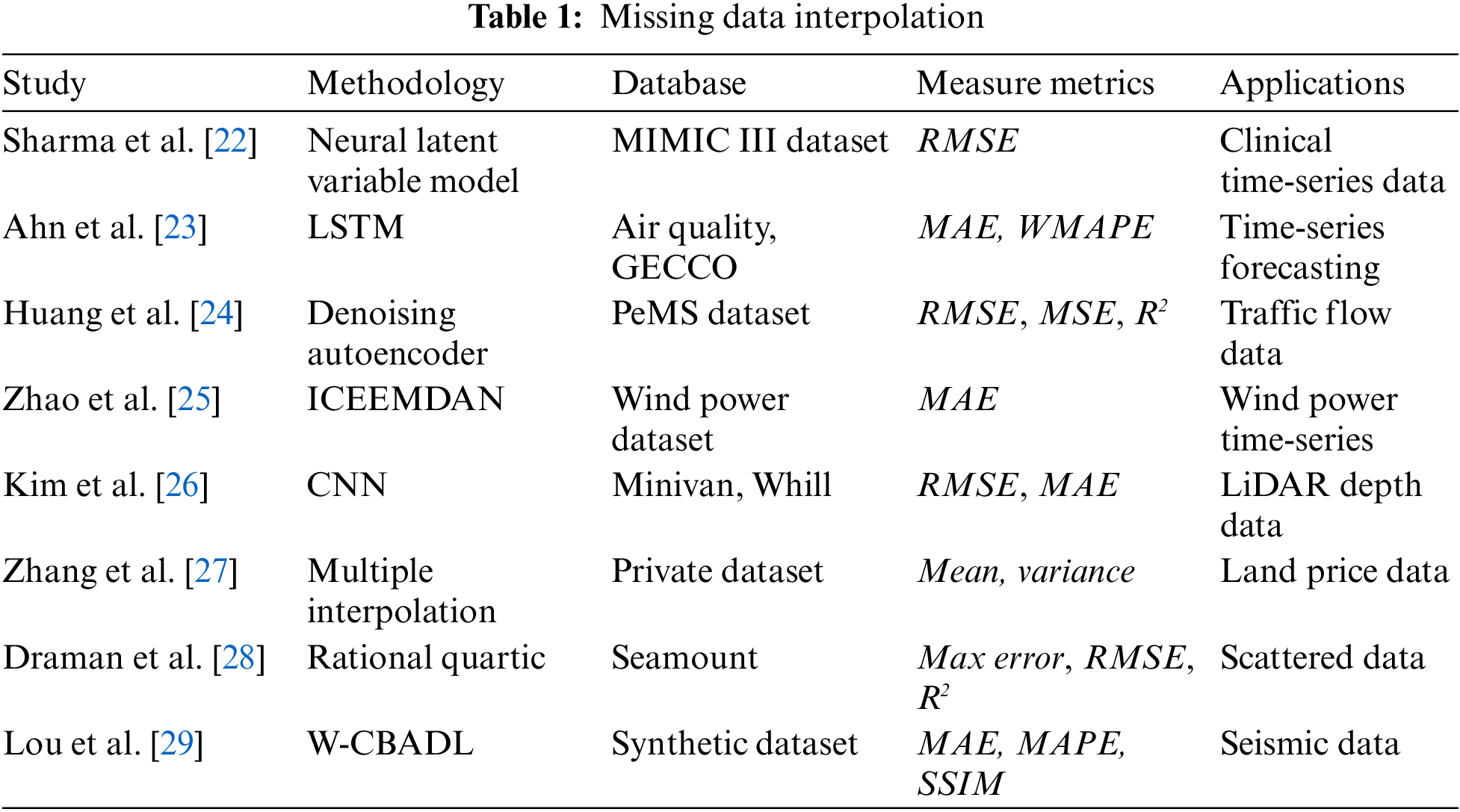
As mentioned in the Introduction, data interpolation which is crucial for timely data analysis or prediction tasks has been widely studied by researchers in various fields. By using a neural latent variable model, known as a Neural Process (NP), Sharma et al. [22] built generative models to estimate missing values in clinical time-series data. Ahn et al. [23] compared and investigated the effects of data imputation methods for building long short-term memory (LSTM) networks-based time series forecasting model, and they used the mean absolute error (MAE) and weighted mean absolute percentage error (WMAPE) as the evaluation metrics. Huang et al. [24] proposed a data interpolation method for traffic generative modeling by applying discrete wavelet transform (DWT) to decompose the complete traffic flow data into low-frequency and high-frequency data. Based on the improved complete ensemble empirical mode decomposition with adaptive noise (CEEMDAN) and generative adversarial interpolation network, Zhao et al. [25] developed a missing interpolation model for wind power data. By establishing a pixelwise dynamic convolution neural network (CNN), Kim et al. [26] performed the interpolation for LiDAR depth data. Using multiple imputation models, Zhang et al. [27] performed data imputation for missing values in land price dataset. Draman et al. [28] applied rational corrected scheme comprising three local schemes defined on each triangle to perform scattered data interpolation, and the metrics including the Root Mean Square Error (RMSE), maximum error (Max error), coefficient of determination (R2) and CPU time (in seconds) are used to evaluate the model performance. Lou et al. [29] proposed a wavelet-based convolutional block attention deep learning network named W-CBADL to implement the interpolation for irregularly sampled seismic data, and they used the metrics such as MAE, MAPE, and structure similarity index measure (SSIM) to evaluate the model performance. Table 1 summarizes the reviewed articles along with their methodologies, databases, measurement metrics, and application fields that focus on missing data interpolation.

3  Materials and Methods

3.1 Materials

The power line loss includes all the power loss from the primary side of the main transformer of the power plant (excluding the power used by the plant) to the user’s electric energy meter. The power line loss cannot be directly measured. It is calculated by subtracting the power supply and the electricity sold. At present, power metering, marketing, business, and decision support systems have basically realized networking and intelligence. It can easily collect, analyze and manage data by using intelligent acquisition terminal equipment and communication network. Relevant data of 1000 10 kV feeder line losses in one year are randomly selected from the power metering system as the research object. The major variables include the object number of 10 kV feeder line loss, voltage level, statistical start time, end time, power input, and power output. Therefore, the line loss rate can be computed as: line loss rate = (supplied power – sold power)/supplied power. Among them, the supplied power is the power collected when entering the line and the sold power is the sum of all the major users’ power consumption on the line. Because the power consumption of individual users such as households is relatively small in a fixed power grid, and be ignored in general, this study primarily focuses on the analysis of the power consumption of large industrial users on the line. Fig. 1 portrays the topology relationship between the large industrial users and lines. It is noteworthy that the electricity consumption of some large users cannot be normally collected due to certain reasons, such as transformer trips, data missing, and terminal parameter setting errors. If this part of the data is lost, the calculation result of the supplied power will be affected, and the daily line loss rate data will eventually lead to a large error. Therefore, it is necessary to interpolate the daily electricity consumption data to achieve a better predictive modeling effect. Table 2 presents the partial sample data.

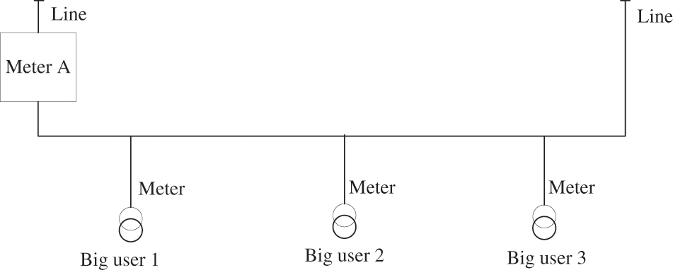
Figure 1: Topological relationship between lines and large users

3.2 Methods

3.2.1 GMDH Algorithm

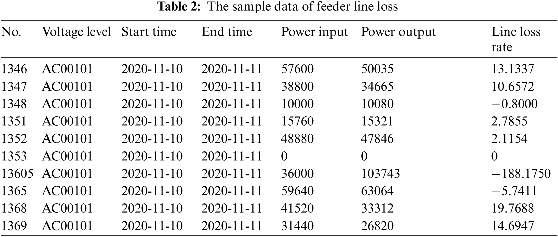
The group method of data handling (GMDH) is a core algorithm of self-organizing data mining, which can automatically determine the variables to enter the model, the model structure and parameters in a self-organizing manner [30–34]. GMDH is essentially a heuristic self-organization algorithm. First, it generates random combinations of input variables based on incomplete information of complex nonlinear systems, and forms multiple combinations named partial descriptions. Then, the optimal combination is selected according to the tentative criteria of adaptability to the external environment. This operation is repeated to form a multi-layer network structure, where each layer includes the formed partial description and selection operation, similar to the process of plant breeding. Finally, the system that can adapt to the external environment is developed automatically, which is termed complete expression. Fig. 2 depicts a typical GMDH network architecture.

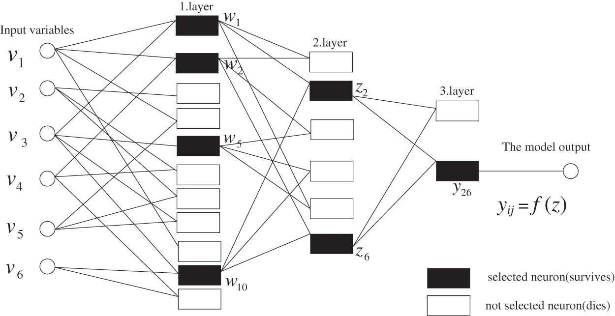
Figure 2: A typical GMDH network

Different from the artificial neural network (ANN) family, GMDH uses the form of mathematical description, namely referential function, to establish the general relationship between the input and output variables for modeling. In general, the Kolmogorov–Gabor (K-G) polynomial [33], which can well represent the mathematical description and model any analytic single-valued transformation through an algebraic sum of terms, is frequently used as the initial model of the algorithm [34]. The K-G polynomial comprised of (v1, v2, ... , vn) variables is established as follows:

y=f(v1,v2,…,vn)=∑i=1naivi+∑i=1n∑j=1naijvivj+∑i=1n∑j=1n∑k=1naijkvivjvk+…(1)

where (v1, v2,..., vn) denotes the input variables, (a1, a2,..., an) means the vector of coefficient or weight, and y is the output variable. Theoretically, as the independent variables and polynomial degree (also known as complexity) increase, a polynomial sequence can fit any numerical data with the required precision [30]. Hence, in practice, this method is often utilized for prediction problems in various domains.

3.2.2 Proposed Approach

First, the dependent and independent variables are defined from the original data set, and the upper and lower limits of missing values are determined according to prior knowledge or existing data information. All missing data are randomly interpolated within the upper and lower limits. Then, the GMDH network of all variables is established to obtain the optimal complexity model, which is used to predict the missing data to replace the last imputed electricity consumption data. Finally, the iterative loop is implemented until the missing values do not change. Fig. 3a portrays the specific processes of the GMDH-based interpolation method, and the details are presented as follows:

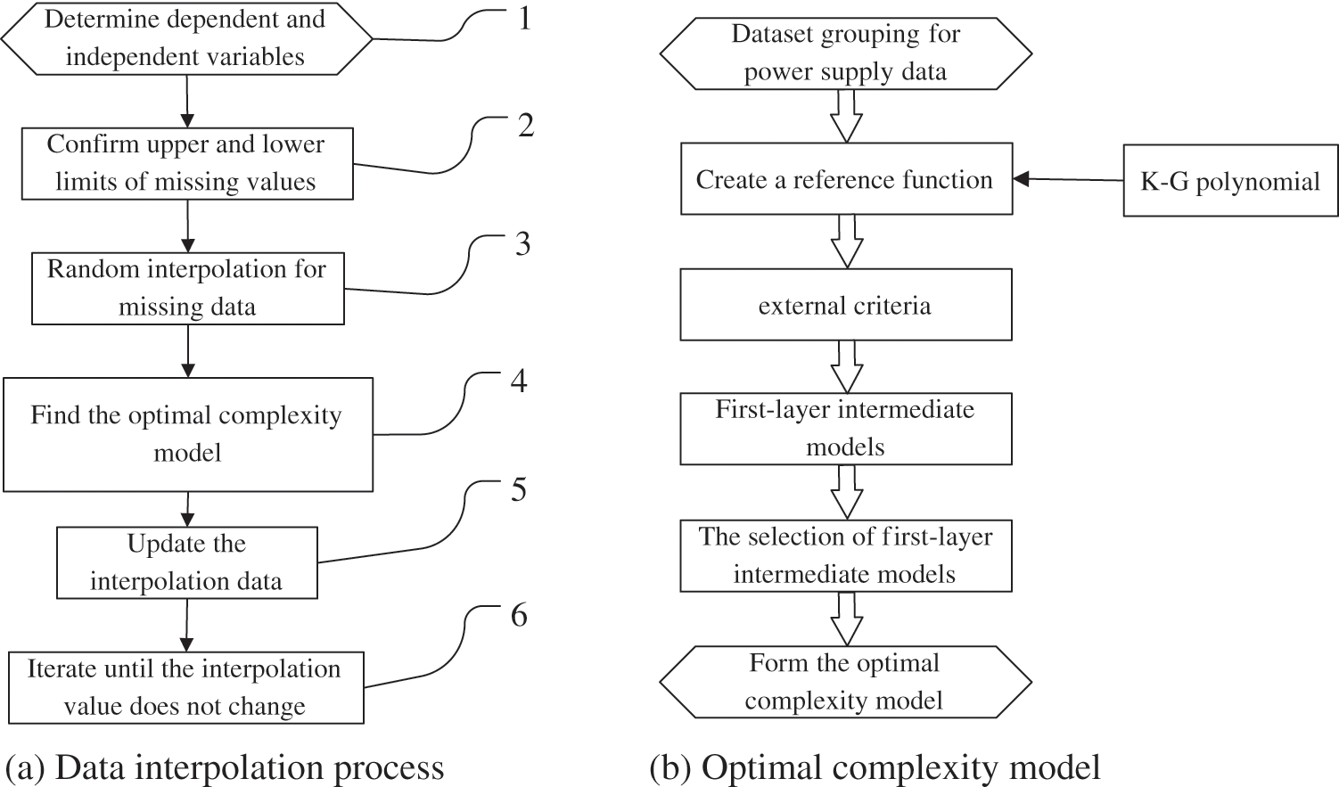
Figure 3: The process of GMDH-based interpolation method

Step 1 (Determine the dependent and independent variables): The variable xi with missing data is determined to be the dependent variable, and the variable (x1, x2, …, xi-1, xi, xi+1, …, xn) without missing data is determined to be the independent variable.

Step 2 (Confirm the upper and lower limits of missing values): According to prior knowledge and existing data information, the upper and lower limits of missing values are counted and designated as [yi_,yi¯]. The value of each iteration does not exceed this range.

Step 3 (Random interpolation for missing data): All missing data are randomly interpolated at the first time, and the interpolated values are located in the interval of [yi_,yi¯].

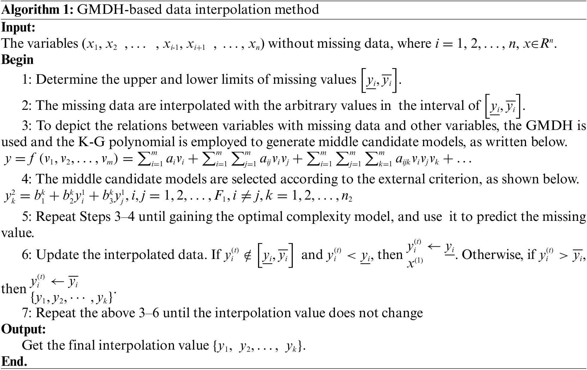
Step 4 (Find the optimal complexity model): This step establishes a GMDH model between variables with missing data and other variables, and finds out the optimal complexity model, as shown in Fig. 3b.

There are two loops in the optimization process: one is the data interpolated by the GMDH algorithm, where the loop is to find the optimum model; the other is to continuously update the filling interpolation value through the loop. Thereafter, the best interpolation value of the model is obtained through the two cycles to improve the accuracy. More specifically, the detailed process of building the optimal complexity model is described as follows:

(1) Divide the electricity consumption data of industrial huge users into training set A and testing set B (Nω=NA+NB,ω=A∪B). Especially, to establish a prediction model, the sampledataset is further divided into a learning set A, validation set B, and testing set C. The ratio of training set, validation set, and test set is 3:1:1, i.e., Nω=NA+NB+NC,ω=A∪B∪C.

(2) The general relationship between dependent variables (variables with missing data) and independent variables (variables without missing data) is established as a “reference function”, where the K-G polynomial is utilized.

(3) Select one or more criteria with the nature of external complementary as the objective function (system), or called external criteria.

(4) Generate the intermediate candidate model of the first layer. The transfer function yk=fk(vi,vj)(k=1,2,…,n) is employed to generate the intermediate candidate models in a self-organizing way, and the number of variables and model structure are different. Whilst, the parameters of yk are estimated on training A.

(5) The selection of the intermediate models in the first layer. Depending upon the external criterion, the first-layer intermediate models are selected on test set B, and the chosen intermediate models ωk(e.g., k=1,2,5,10) are used as the input variables of the second layer.

(6) Form the optimal complexity model. Repeating the above (4) and (5), the intermediate candidate models of the second to nth layers can be yielded in turn, and finally, the optimal complexity model that can be analyzed and explicit is formed.

Step 5 (Update the interpolation data): The value calculated by the optimal complexity model is used to replace the last interpolation value of the missing data. If the calculated value of a certain iteration exceeds the upper and lower limits, the boundary value is used to interpolate the missing data. Mathematically, in the ith iteration, if yi(t)∉[yi_,yi¯] and yi(t)<yi_, then yi(t)←yi_. Otherwise, if yi(t)>yi¯, then yi(t)←yi¯.

Step 6 (Iterate until the interpolation value does not change): Repeat the above processes from step 3 to step 5 until the interpolation value of the iteration does not change anymore. In summary, a brief description of the above processes is presented in Algorithm 1.

4  Experiments

To verify the validity of the proposed approach, this paper uses the actual data collected from the line loss module of the electric energy metering automation system as the analysis object. A real-world empirical study was performed using the proposed GMDH-based data interpolation method for missing electricity consumption data imputation in power supply bureaus of Guangxi, China. Table 3 summarizes the representative sample data, and each row of the original data in this table represents the electricity quantity collected at 10 time points a day. Where the electricity quantity series x of a certain day contains missing data, and the data of the electricity quantity series y of the previous day is complete at the same time. Note that 2 data are missing in 20 sets of data and the missing rate is 10%. Therefore, using the proposed GMDH-based data interpolation method, the missing data are iteratively interpolated and the error rate between the interpolated data and the original data is compared under different noise levels.

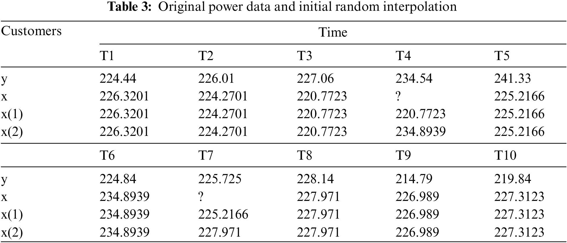
Firstly, all missing data are randomly interpolated, and the interpolated values are located in the interval of [yi_,yi¯]. For example, the nearest data to the missing value x are 220.7723 and 225.2166 when y is equal to 234.54, as shown in Table 3. The first interpolation of missing data for x uses the random value located in the range of [220.772 3225.216 6], and similarly, the nearest values of the second missing data are 234.8939 and 227.971, respectively. The nearest neighbor values can be randomly selected to interpolate into the missing data, and it can be taken as the initial scheme of the next interpolation. By doing this, the data used for each interpolation is the intermediate data of the interval, which ensures that the interpolated value will not exceed the initial upper and lower limits. Subsequently, this study establishes the GMDH model between the variables with missing data and other variables, and finds out the optimal complexity model. The K-G polynomial is selected as the reference function, and to simplify the algorithm, the initial function selected in this experiment is as follows:

y=f(x)=1.5x1+2x2−3x3+2.5x4−0.7x5+1.1x6(2)

where x1~x6 are the 6 samples with the smallest distance (k = 6). In addition, the system is susceptible to various noise disturbances, such as power reading errors, measurement errors, and various objective factors. Therefore, considering the noise interference, the actual observed sample data conforms to the following relationship:

y=f(x)+αZ(3)

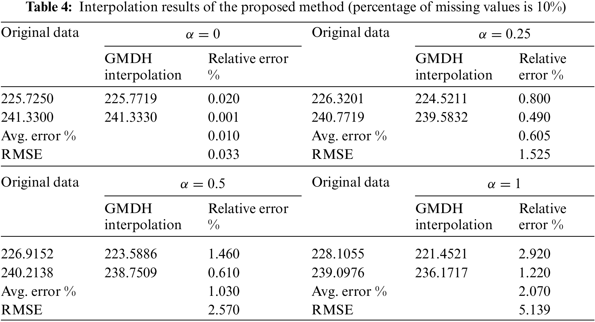
In Eq. (3), the value of α is in (0, 0.25, 0.5, 1), Z is 4 groups of random data located in the interval [−0.5, 0.5], and α is equal to 0 when the system is not disturbed by noises. The x value under different noise levels is compared with the data interpolated by the GMDH method, and the Z value of each simulation is randomly generated by the computer. Table 4 displays the results of the GMDH-based data interpolation method with the 10% percentage of missing data. Considering the measurement of model efficiency, we investigate the performance using the metrics like the relative error (Erel) and root mean squared error (RMSE), which are correspondingly calculated in Eqs. (4) and (5).

Erel=|y^i−yi|yi×100%(4)

RMSE=1n∑i=1n(yi−y^i)2(5)

where yi and y^i stand for the actual value and predicted value, respectively. It can be observed from Table 4 that the calculation error of the proposed method is relatively small, and the maximum error does not exceed 0.605% at relatively small noise levels (e.g., α = 0.25), which demonstrates that the proposed method can effectively perform the interpolation for the missing data and has a certain anti-interference ability.

Moreover, Table 5 presents the results of the GMDH-based data interpolation method with a higher percentage of missing data (30%). From Table 5, it can be seen that when the missing rate of the collected data is high, the GMDH-based data interpolation method can also be used to estimate the missing data and obtain a relatively low error rate. Therefore, the model can be deployed to the electricity metering system and applied to the power line loss analysis as well as other functional modules that require high-quality data. It provides a basis for business applications such as power line loss analysis of the metering automation system. A comparative analysis of the line loss rate (LLR) on a certain line before and after data interpolation is shown in Table 6, and the corresponding curve is depicted in Fig. 4.

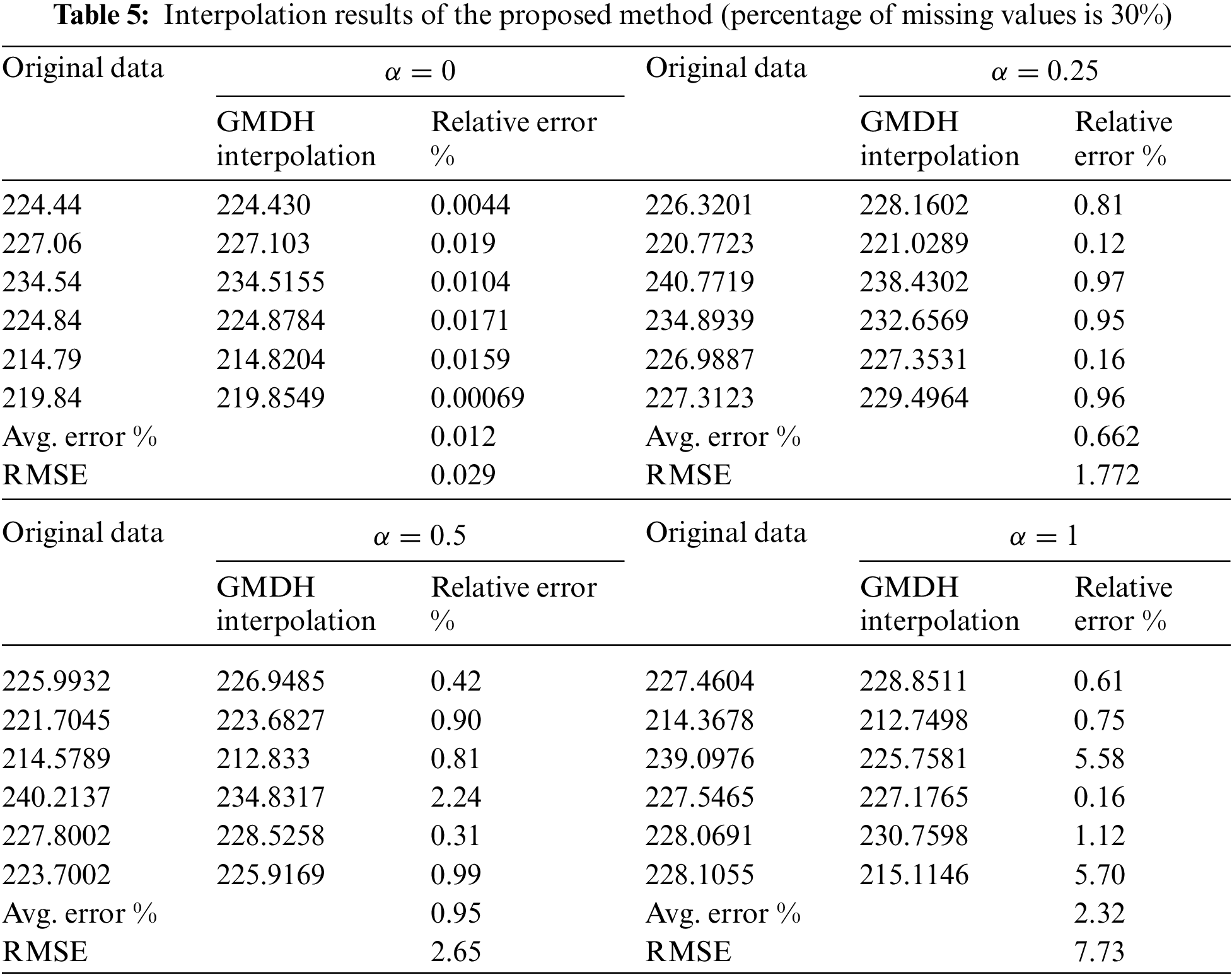
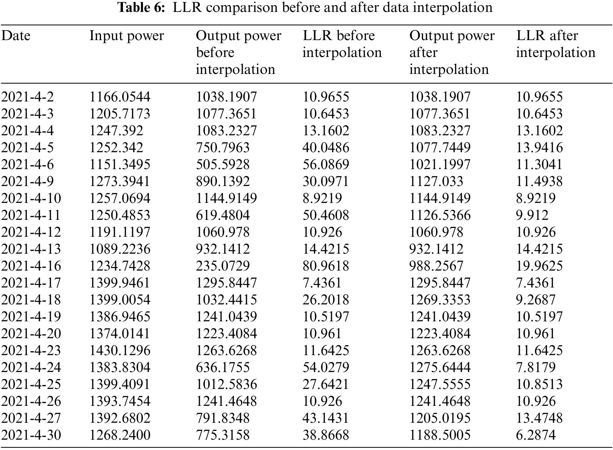
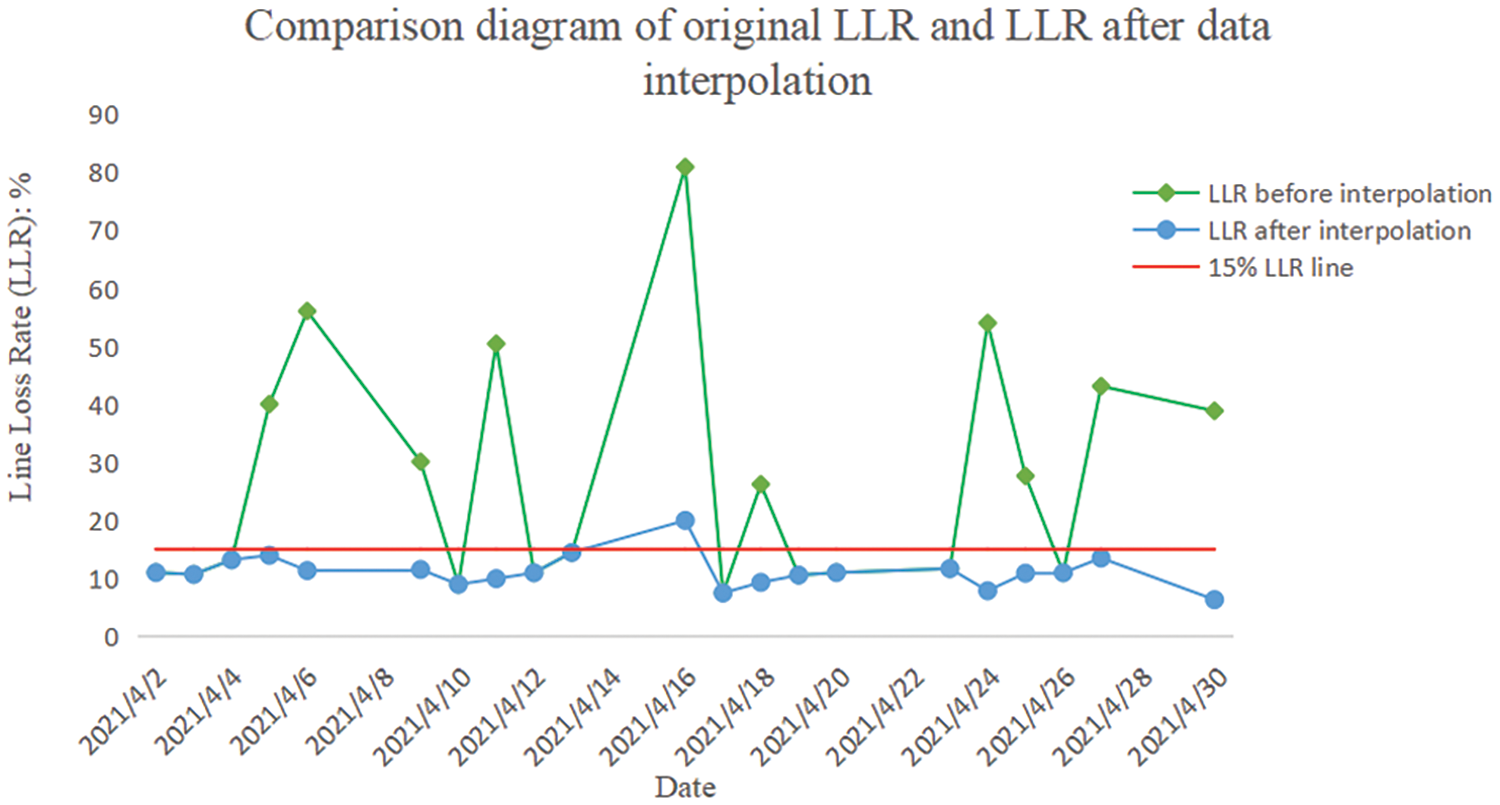
Figure 4: LLR comparison before and after interpolation

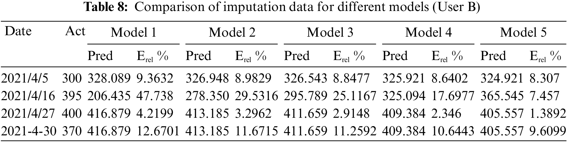
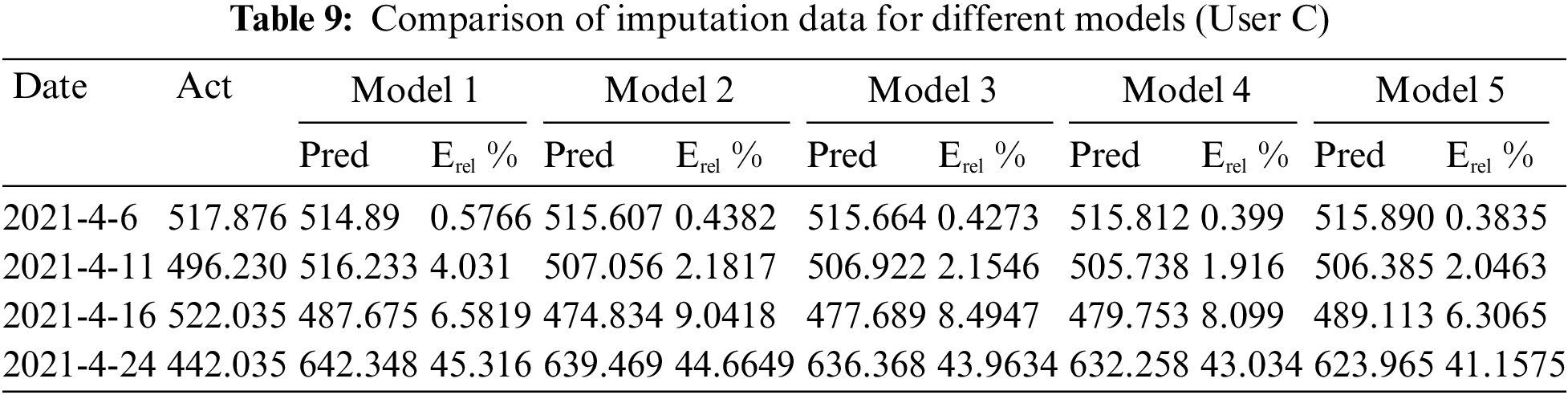
It can be seen from Fig. 4 that the data of many days before interpolation can be considered as the line loss rate exceeding the standard (more than 15%), or even seriously exceeding the standard (more than 30%). Thus, the suspicion of electricity theft is relatively high on this line. However, the fact is that the electricity consumption data on this line has not been recorded, which causes the poor prediction effect of the models. From the curve of LLR after interpolation, it can be observed that the line loss rate exceeding the standard is only on 2021-4-16, indicating that many original missing data have been interpolated. As a result, the line loss rate has decreased and this is more in line with the normal situation. In addition, considering different noise levels, e.g., α = 1.0, 0.6, 0.5, 0.33, and 0.1, the 5 models with different α parameters are used to interpolate the missing electricity quantity data of different users. The comparison results of different models are presented in Tables 7–9, respectively.

According to the results predicted in the above tables, the total errors of these five models are 134.4196, 113.5041, 106.8864, 96.6144, and 80.8589, respectively. Whilst, depending upon the electricity quantity value predicted by different models, the corresponding power line loss rates are calculated, respectively. Table 10 summarizes the power line loss rate statistics based on the prediction results of different models, and the corresponding curve is depicted in Fig. 5.

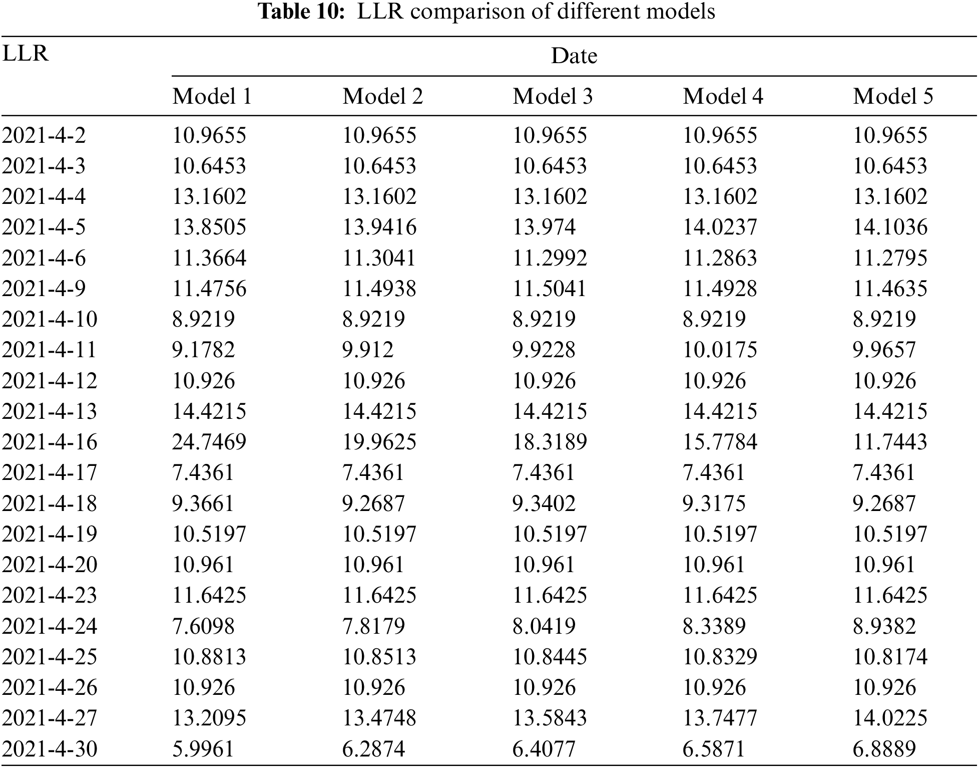
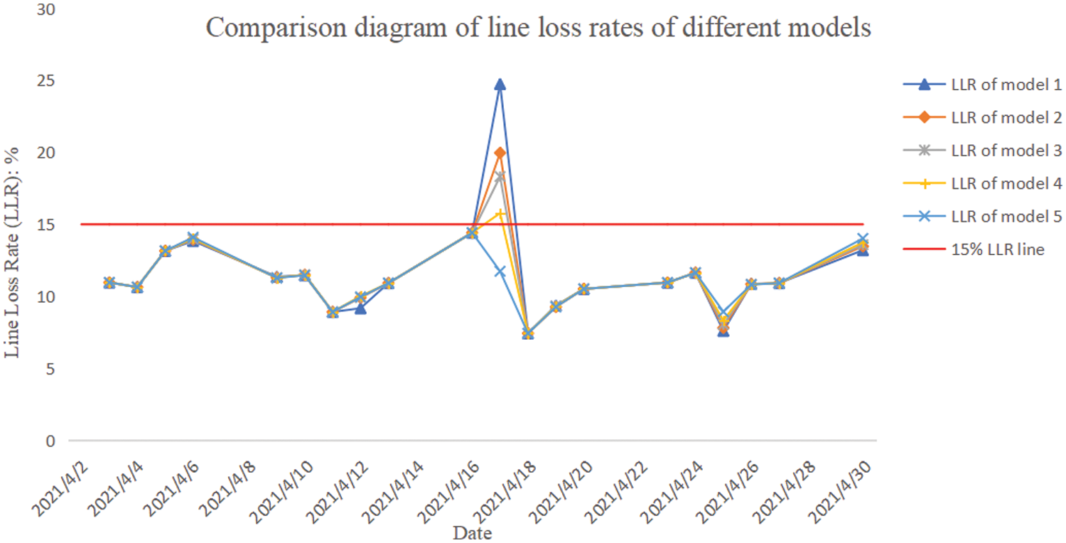
Figure 5: LLR comparison diagram of different models

From the comparison of electricity prediction errors of different models in Table 10, it can be assumed that model 1 has the largest deviation owing to the influence of relatively high noise levels. Also, it can be observed from the LLR comparison chart of different models in Fig. 5 that the curve of model 1 has the largest fluctuation range, which indicates the relatively large errors of this model. On the contrary, model 5 has the smallest prediction error of electricity quantity and the LLR curve almost coincides with other curves, which implies the overfitting risks of this model. Therefore, we remove these two models in the interpolation analysis of missing electricity consumption data.

5  Conclusion

In intelligent power management, such as adaptive anti-theft diagnosis modeling, there are evaluation indicators like power, load, alarm, and line loss, and the data quality of these evaluation indicators is very important and will affect the accuracy of the modeling results. Due to network packet loss, terminal failure, electricity cut, and other factors, some metering points may be offline or data cannot be collected in the power metering system, resulting in missing and incomplete data. The lack of electricity data not only affects the collection integrity rate, average electricity consumption, electronic marketing settlement, and other utility indexes but also influences the effectiveness of the electricity theft diagnosis and metering device fault detection. Thereupon, to address these challenges, this paper proposes a GMDH-based data interpolation method for missing electricity consumption data. The upper and lower limits of missing values are initially determined according to prior knowledge or existing data information, and the missing data were randomly interpolated within the upper and lower limits. Then, the GMDH network with multiple variables as the input is established to gain the optimal complexity model, which is used to predict the missing value to replace the last interpolated dataiteratively.

The empirical analysis result shows that the calculation error of the proposed approach is relatively small, demonstrating the efficacy and feasibility of the proposed approach. It has successfully updated the missing electricity consumption data, automatically realized the organization and management of data, and offered the basis for the analysis of abnormal electricity consumption, such as electricity theft, illegal power utilization, metering device faults and errors. In future development, we expect to embed the model into the electricity metering system to automatically interpolate the values for the missing electricity consumption data. Meanwhile, this approach can be transplanted to other related fields, such as data exception processing, online prediction analysis, sparse signal recovery, and others.

Acknowledgement: The work is partially supported by the Research Funds of Hunan Provincial Natural Science Research Fund. The authors would also like to thank the editors and unknown reviewers for their constructive advice.

Funding Statement: This research was funded by the National Nature Sciences Foundation of China (Grant No. 42250410321).

Author Contributions: J.C., Y.J., and W.C.: data collection, analysis, and interpretation of results, draft manuscript preparation; M.C.S., and Y.A.N.: supervision, visualization and revise the manuscript. All authors reviewed the results and approved the final version of the manuscript.

Availability of Data and Materials: The datasets used and/or analyzed during the current study are available from the corresponding author on reasonable request.

Conflicts of Interest: The authors declare that they have no conflicts of interest to report regarding the present study.

References

1. S. Li and F. Yang, “Research on abnormal line loss data system in power grid through abnormal identification of line loss index,” in 2021 IEEE Int. Conf. Data Sci. Comput. Appl. (ICDSCA), 2021, pp. 102–106. [Google Scholar]

2. J. Chen, A. Zeb, Y. Sun, and D. Zhang, “A power line loss analysis method based on boost clustering,” J. Supercomput., vol. 79, pp. 3210–3226, 2023. doi: 10.1007/s11227-022-04777-w. [Google Scholar] [CrossRef]

3. X. Wang, H. Fan, T. Wang, X. Yang, and K. Zhang, “The analysis method of line loss for planning grid,” in 2012 Asia-Pac. Power Energy Eng. Conf., 2012, pp. 1–5. [Google Scholar]

4. K. Liu et al., “Research on diagnosis of abnormal line loss of 10kV transmission line based on factor analysis,” in 2021 IEEE Int. Conf. Power, Intell. Comput. Syst. (ICPICS), 2021, pp. 371–374. [Google Scholar]

5. J. Chen, D. Zhang, and Y. A. Nanehkaran, “Research of power load prediction based on boost clustering,” Soft Comput., vol. 25, pp. 6401–6413, 2021. doi: 10.1007/s00500-021-05632-5. [Google Scholar] [CrossRef]

6. T. Nagayama and F. S. Billie Spencer Jr, “Structural health monitoring using smart sensors,” Univ. of Illinois at Urbana-Champaign, Newmark Struct. Eng. Lab., USA, 2007. [Google Scholar]

7. Q. Lin, X. Bao, and C. Li, “Deep learning based missing data recovery of non-stationary wind velocity,” J. Wind. Eng. Ind. Aerodyn., vol. 224, pp. 104962, 2022. doi: 10.1016/j.jweia.2022.104962. [Google Scholar] [CrossRef]

8. E. Luedeling, K. Achim, and M. M. Blanke, “Identification of chilling and heat requirements of cherry trees—A statistical approach,” Int. J. Biometeorol., vol. 57, no. 5, pp. 679–689, 2013. doi: 10.1007/s00484-012-0594-y. [Google Scholar] [PubMed] [CrossRef]

9. J. Oteros, C. Carmen, A. Purificación, and E. Domínguez-Vilches, “Quality control in bio-monitoring networks, Spanish Aerobiology Network,” Sci. Total Environ., vol. 443, pp. 559–565, 2013. doi: 10.1016/j.scitotenv.2012.11.040. [Google Scholar] [PubMed] [CrossRef]

10. A. Ngueilbaye, H. Wang, D. A. Mahamat, and S. B. Junaidu, “Modulo 9 model-based learning for missing data imputation,” Appl. Soft Comput., vol. 103, pp. 107167, 2021. doi: 10.1016/j.asoc.2021.107167. [Google Scholar] [CrossRef]

11. X. Miao, Y. Wu, L. Chen, Y. Gao, and J. Yin, “An experimental survey of missing data imputation algorithms,” IEEE Trans. Knowl. Data Eng., vol. 35, no. 7, pp. 6630–6650, 2022. doi: 10.1109/TKDE.2022.3186498. [Google Scholar] [CrossRef]

12. W. L. Junger and A. P. de Leon, “Imputation of missing data in time series for air pollutants,” Atmos. Environ., vol. 102, pp. 96–104, 2015. doi: 10.1016/j.atmosenv.2014.11.049. [Google Scholar] [CrossRef]

13. L. Guo, J. Dai, S. Ranjitkar, H. Yu, J. Xu and E. Luedeling, “Chilling and heat requirements for flowering in temperate fruit trees,” Int. J. Biometeorol., vol. 58, pp. 1195–1206, 2014. doi: 10.1007/s00484-013-0714-3. [Google Scholar] [PubMed] [CrossRef]

14. Y. Gong, Z. Li, J. Zhang, W. Liu, Y. Yin and Y. Zheng, “Missing value imputation for multi-view urban statistical data via spatial correlation learning,” IEEE Trans. Knowl. Data Eng., vol. 35, no. 1, pp. 686–698, 2021. doi: 10.1109/TKDE.2021.3072642. [Google Scholar] [CrossRef]

15. V. Todorov, “rrcovNA: Scalable robust estimators with high breakdown point for incomplete data,” R package version 0.4-15, 2020. [Google Scholar]

16. S. Zhang, “Nearest neighbor selection for iteratively kNN imputation,” J. Syst. Softw., vol. 85, no. 11, pp. 2541–2552, 2012. doi: 10.1016/j.jss.2012.05.073. [Google Scholar] [CrossRef]

17. Z. Yang, Y. Liu, and C. Li, “Interpolation of missing wind data based on ANFIS,” Renew. Energy, vol. 36, no. 3, pp. 993–998, 2011. doi: 10.1016/j.renene.2010.08.033. [Google Scholar] [CrossRef]

18. B. Fallah, K. T. W. Ng, H. L. Vu, and F. Torabi, “Application of a multi-stage neural network approach for time-series landfill gas modeling with missing data imputation,” Waste Manag., vol. 116, pp. 66–78, 2020. doi: 10.1016/j.wasman.2020.07.034. [Google Scholar] [PubMed] [CrossRef]

19. J. Nan, Y. Li, H. Zuo, H. Zheng, and Q. Zheng, “BiLSTM-A: A missing value imputation method for PM2. 5 prediction,” in 2020 2nd Int. Conf. Applied Mach. Learn. (ICAML), 2020, pp. 23–28. [Google Scholar]

20. D. J. Stekhoven and P. Bühlmann, “MissForest—Non-parametric missing value imputation for mixed-type data,” Bioinform., vol. 28, no. 1, pp. 112–118, 2012. doi: 10.1093/bioinformatics/btr597. [Google Scholar] [PubMed] [CrossRef]

21. A. Picornell et al., “Methods for interpolating missing data in aerobiological databases,” Environ. Res., vol. 200, pp. 111391, 2021. doi: 10.1016/j.envres.2021.111391. [Google Scholar] [PubMed] [CrossRef]

22. P. Sharma, F. E. Shamout, V. Abrol, and D. A. Clifton, “Data pre-processing using neural processes for modeling personalized vital-sign time-series data,” IEEE J. Biomed. Health Inform., vol. 26, no. 4, pp. 1528–1537, 2021. doi: 10.1109/JBHI.2021.3107518. [Google Scholar] [PubMed] [CrossRef]

23. H. Ahn, K. Sun, and K. P. Kim, “Comparison of missing data imputation methods in time series forecasting,” Comput. Mater. Contin., vol. 70, no. 1, pp. 767–779, 2022. doi: 10.32604/cmc.2022.019369. [Google Scholar] [CrossRef]

24. Y. Huang and F. Chen, “Data interpolation of traffic flow algorithm using wavelet transform for traffic generative modeling,” IEEE J. Radio Freq. Identif., vol. 6, pp. 739–742, 2022. doi: 10.1109/JRFID.2022.3217084. [Google Scholar] [CrossRef]

25. L. Zhao et al., “Missing interpolation model for wind power data based on the improved CEEMDAN method and generative adversarial interpolation network,” Global Energy Intercon., vol. 6, no. 5, pp. 517–529, 2023. doi: 10.1016/j.gloei.2023.10.001. [Google Scholar] [CrossRef]

26. W. Kim, M. Tanaka, M. Okutomi, and Y. Sasaki, “Pixelwise dynamic convolution neural network for LiDAR depth data interpolation,” IEEE Sens. J., vol. 21, no. 24, pp. 27736–27747, 2021. doi: 10.1109/JSEN.2021.3124325. [Google Scholar] [CrossRef]

27. L. Zhang, L. Bai, X. Zhang, Y. Zhang, F. Sun and C. Chen, “Comparative variance and multiple imputation used for missing values in land price dataSet,” Comput. Mater. Contin., vol. 61, no. 3, pp. 1175–1187, 2019. doi: 10.32604/cmc.2019.06075. [Google Scholar] [CrossRef]

28. N. N. C. Draman, S. A. A. Karim, and I. Hashim, “Scattered data interpolation using rational quartic triangular patches with three parameters,” IEEE Access, vol. 8, pp. 44239–44262, 2020. doi: 10.1109/ACCESS.2020.2978173. [Google Scholar] [CrossRef]

29. Y. Lou et al., “Irregularly sampled seismic data interpolation via wavelet-based convolutional block attention deep learning,” Artif. Intell. Geosci., vol. 3, pp. 192–202, 2022. doi: 10.1016/j.aiig.2022.12.001. [Google Scholar] [CrossRef]

30. J. A. Mueller and F. Lemke, Self-Organising Data Mining: An Intelligent Approach to Extract Knowledge From Data. Hamburg: Libri, 2000. [Google Scholar]

31. J. Chen, S. Yang, D. Zhang, and Y. A. Nanehkaran, “A turning point prediction method of stock price based on RVFL-GMDH and chaotic time series analysis,” Knowl. Inf. Syst., vol. 63, no. 10, pp. 2693–2718, 2021. doi: 10.1007/s10115-021-01602-3. [Google Scholar] [PubMed] [CrossRef]

32. C. Z. He, J. Wu, and J. A. Müller, “Optimal cooperation between external criterion and data division in GMDH,” Int. J. Syst. Sci., vol. 39, no. 6, pp. 601–606, 2008. doi: 10.1080/00207720701750816. [Google Scholar] [CrossRef]

33. A. R. Barron and R. L. Barron, “Statistical learning networks: A unifying view,” in Symposium on the Interface: Statistics and Computing Science, Apr. 1998, pp. 21–23. [Google Scholar]

34. X. Jin, C. He, and S. Wang, “A classifier ensemble model based on GMDH-type neural network for customer targeting,” in Proc. Seventh Int. Conf. Manag. Sci. Eng. Manag., Berlin, Heidelberg, Springer, 2014, pp. 259–269. [Google Scholar]