Boosting Adversarial Training with Learnable Distribution

1  Introduction

In recent years, the rapid advancement of Deep Neural Networks (DNNs) has led to their extensive application, including computer vision [1,2], audio recognition [3], and natural language processing [4,5]. However, DNN models are vulnerable to adversarial examples [6], where slight modifications in input data can lead to incorrect predictions. This raises serious security concerns, particularly in safety-critical applications such as image classification [7], object detection [8,9] and autonomous driving [10].

To address these challenges, various defensive approaches have been proposed [11–13] to respond to the emergence of adversarial attacks. Adversarial training [14–17] has gained more attention, and is being considered as the most effective defense method among others. This method involves training a DNN model by using both natural and adversarial examples. Thus, the model learns to generalize in the presence of adversarial examples. The adversarial training introduced by Madry et al. [14] involves natural examples with adversarial examples generated through the projected gradient descent (PGD) attack. Their study enhanced the models’ ability to defend against adversarial attacks by pushing the predicted label of adversarial examples closer to the ground-truth. However, their study did not consider natural accuracy. Regularization-based adversarial training methods [6,18,19] have also been proposed to improve DNN robustness. These methods often face a trade-off between robust and natural accuracy, using regularization terms such as Kullback–Leibler (KL) divergence and logit pairing [19]. However, they overlooked the variations in the distribution of natural and adversarial examples.

Previous studies [20,21] have revealed that natural and adversarial examples have distinct underlying distributions. Strengthening the model’s consistency for both types of examples may result in a decline in the accuracy of natural examples. As shown in Fig. 1a, the model accurately classifies natural examples (blue dots) but struggles to classify the corresponding adversarial examples (red dots). Existing adversarial training methods [18,19] aim to ensure consistency between model output for natural and adversarial examples. The model successfully classifies most adversarial examples, as shown in Fig. 1b. However, this causes natural examples to move closer to or even cross the decision boundary, resulting in decreased model accuracy. The proposed method encourages both natural and adversarial examples to be close to the same distribution centroid. As shown in Fig. 1c, both natural and adversarial samples follow the same distribution. Each distribution contains a distribution centroid represented by yellow dots. Assuming that natural and adversarial examples originate from distinct underlying distributions within the feature space, the task for a model to classify them as belonging to the same class poses significant challenges, hence our motivation.

Figure 1: Illustration of the decision boundary of the (a) Natural model, (b) Existing robust model, and (c) Our robust model. Different shapes represent the expected features of images in various classes

The proposed method aimed to bring natural and adversarial examples closer to the distribution centroid of the ground-truth class in the feature space. This is achieved by acquiring a robust distribution centroid through gradient back-propagation using both natural and adversarial examples. This method also allows for rejecting the classification of samples far from the distribution centroid. A Gaussian mixture model is used as a classifier to capture the feature distribution of the input. Samples close to the distribution centroid have a higher confidence, which complements the robustness of the model. The main contributions of this work involve the following aspects:

•   The distribution gap between natural and adversarial examples in the feature space is closed, leveraging the learnable classification centroid to guide adversarial training.

•   A decision-boundary-based adversarial attack algorithm is proposed for adversarial training, which can generate adversarial examples close to the natural example distribution while minimizing excessive distribution differences.

•   Adversarial examples are detected by analyzing the likelihood estimation of the model output. This two-stage defense method allows a few adversarial examples to bypass the defense mechanism.

The remainder of this paper is structured as follows. Section 2 describes the related work. Section 3 describes the proposed adversarial training method, including feature modeling and the pipeline for adversarial example generation and training. In Section 4, numerous experiments are conducted, and the potential uses of probability estimation for deployment are discussed, and finally, Section 5 describes the conclusion of the paper.

2  Related Work

2.1 Adversarial Attack

Since the advent of adversarial examples, a wide range of attack methods to generate adversarial examples have been explored. Adversarial examples can readily fool DNNs in real-world circumstances, thus becoming a major hurdle to DNN implementation. Nevertheless, this is worth investigating, as the existence of adversarial attacks may accelerate the progress of the work on adversarial defense.

2.1.1 Fast Gradient Sign Method (FGSM)

Goodfellow et al. [6] proposed a fast way to generate adversarial examples known as the fast gradient sign method (FGSM). FGSM generates a one-step perturbation along the gradient of the loss function concerning the natural image x.

x′=x+ϵsign(∇xL(θ,x,y)).(1)

This equation computes the adversarial input x′, obtained by adding a slight perturbation ϵ to the original input x. This perturbation is proportional to the sign of the gradient of the model’s loss function L(θ,x,y) concerning the input features x, where y denotes the true label of the input.

2.1.2 Projected Gradient Descent (PGD)

Madry et al. [14] proposed a multi-step attack method termed projected gradient descent (PGD). PGD generates the perturbation iteratively with small steps from a randomly initialized point around the natural example and constrains the adversarial perturbation under the Lp−norm constraint:

x0′=x,xt+1′=Π∥x′−x∥p≤ϵ(xt′+αsign(∇xt′L(fθ(xt′),y))).(2)

where Π(.) represents the projection operator, t denotes the current step, α denotes the step size, and ϵ represents the magnitude of perturbation.

2.1.3 Carlini & Wagner (C&W)

Carlini et al. [22] proposed the C&W attack, which directly optimizes the L2 regularization term and the difference between logits. The untarget attack version of C&W can be expressed as:

minδ[∥x~−x∥22−Cfθ(x~)],fθ(x~)=max(maxi≠y⁡{Z(x~)i}−Z(x~)y,−k),x~=12(tanh(arctanh(x)+δ)+1).(3)

where Z(.)i is the model output before the softmax, k denotes a confidence control parameter. The C&W attack has outstanding transferability and high confidence.

2.2 Adversarial Defense

Several methods for adversarial defense have emerged after the discovery of the adversarial example. Among them, adversarial training has become the common defense method against adversarial attacks. Existing adversarial training methods can be categorized into three groups: PGD adversarial training, regularization-based adversarial training and curriculum learning-based adversarial training.

2.2.1 PGD Adversarial Training

Madry et al. [14] suggested using a PGD attack for adversarial training. Madry et al. [14] formalized adversarial training as a min-max optimization problem:

minθ⁡ρ(θ),ρ(θ)=1n∑i=1n(maxL(fθ(xi′),yi)).(4)

where x′ represents the adversarial example in the Lp-ball around the natural example x.

2.2.2 Regularization-Based Adversarial Training

Kannan et al. [19] proposed logit pairing to promote similarity between the logits of a natural example and its corresponding adversarial example. Zhang et al. [18] proposed that misclassifications stem from both the classification error and the boundary error. Boundary error indicates the closeness of the input features to the decision boundary. In addition to PGD adversarial training, Zhang et al. [18] balanced the trade-off between robustness and accuracy by minimizing the loss of the two parts:

minθ⁡ρ(θ),ρ(θ)=1n∑i=1n(L(fθ(xi),yi)+βmaxKL(fθ(xi)∥fθ(xi′))).(5)

where KL represents the divergence, L represents the classification loss, and β balances accuracy and robustness.

2.2.3 Curriculum Learning-Based Adversarial Training

The min-max formulation always attempts to find the worst-case samples, but it sometimes hurts the natural generalization. Some researchers have introduced the concept of curriculum learning to adversarial training, which avoids selecting worst-case samples. Cai et al. [23] proposed curriculum adversarial training (CAT), which gradually increases the number of iteration steps of PGD attacks during the training period. Cai et al. suggested that adversarial examples generated by strong attacks lead to overfitting during adversarial training. Zhang et al. [24] proposed friendly adversarial training (FAT) by utilizing early stopping during PGD to generate adversarial examples that have just crossed the decision boundary for training.

3  The Proposed Method

Existing adversarial training methods use loss functions to guide the model to extract more robust latent features, but do not impose explicit constraints on the feature distribution. In this paper, the distribution of samples in the feature space is constrained to narrow the distribution gap between natural and adversarial examples.

It is argued by this paper that different underlying distributions are exhibited by natural and adversarial examples. The difference in the distribution is not eliminated for natural and adversarial examples, even if the same labels are assigned or various regularization terms are applied. As shown in Fig. 2a, there are inherent distribution differences between natural and adversarial examples.

Figure 2: Comparison between (a) sample feature distribution of existing methods and (b) sample feature distribution of the proposed method. The inherent difference between existing methods and the proposed method, where the proposed method aligns both natural and adversarial examples to the same distribution

In this paper, a learnable distribution adversarial training method (LDAT) is proposed to narrow the gap in the feature distribution between natural and adversarial examples. As shown in Fig. 2b, natural and adversarial examples both follow the same distribution in the proposed method. However, natural examples are closer to the distribution centroid than adversarial examples. This is consistent with human intuition that natural examples are closer to the classification centroid than adversarial examples, resulting in the model making classifications with increased confidence.

The features of the samples are modeled in Section 3.1, and the adversarial attack algorithm that generates samples for adversarial training is introduced in Section 3.2. Finally, the complete training process for LDAT is summarized in Section 3.3.

3.1 Feature Modeling

The distribution centroid is obtained from the distribution by modeling the latent features of the samples as described in Section 1. The Gaussian mixture model is used for classification instead of fully connected layers. For a K-classification problem, given a dataset (xi,yi)i=1,…,n with xi∈Rd as a natural example and yi∈{1,…,K} as its corresponding label. Each class in the Gaussian mixture model has a Gaussian component. Therefore, the posterior probability of the ground-truth label yi can be expressed as:

p(yi∣xi)=𝒩(hθ(xi);μyi)∑k=1K𝒩(hθ(xi);μk).(6)

where hθ(.) represents the process of extracting features in the neural network, 𝒩(.) is the probability density function of the Gaussian distribution. μk represents the Gaussian mean of class K, which is the distribution centroid for each class.

For the setup of the Gaussian mixture model, the covariance matrix of the Gaussian mixture model is set to the identity matrix, and the prior probability of each class is set to 1/K. The classification margin and likelihood regularization to improve the extra intra-class compactness and inter-class separability of the model. Ignoring the constant term and constant coefficient, the term for likelihood regularization can be formulated as:

ℒlkd=1N∑i∥hθ(xi)−μyi∥2.(7)

The likelihood regularization term serves as a constraint on the sample feature distribution. In the proposed method, the likelihood regularization term aims to align the training data with the assumed Gaussian distribution. It drives both natural and adversarial examples closer to the distribution centroid for the corresponding class.

3.2 Adversarial Example for Adversarial Training

Recent studies based on curriculum learning [23–25] have suggested that adversarial examples near the decision boundary are more beneficial for adversarial training compared to strong adversarial examples. When adversarial examples significantly cross the decision boundary, it is difficult for the proposed method to find the exact distribution centroid. At the same time, it is not beneficial to narrow the distribution gap between the natural and adversarial examples.

When the accuracy and robustness of the model are low, it will be misclassified without introducing any perturbation or with only a small amount of perturbation. As the model’s robustness improves, the sample requires a larger perturbation to cross the decision boundary. As discussed above, to gradually improve the robustness of the model, the magnitude of the perturbation is set based on the decision boundary.

For the proposed adversarial training method, an adversarial attack based on a decision boundary is introduced in this paper. The complete algorithm, encompassing all steps and procedures, is presented in Algorithm 1. Adversarial examples can be studied over a larger range by controlling the perturbation magnitude. The loss function used in the proposed adversarial attack algorithm is cross-entropy.

To avoid overfitting the model to a particular attack, it is important to identify more general perturbations. The proposed attack algorithm searches for adversarial examples in a larger range to determine a more optimal perturbation direction. The attack algorithm only clips the perturbation at the end of the iteration.

A binary classification problem was considered in this paper to offer a comprehensive understanding of the proposed adversarial attack method, as shown in Fig. 3. Let x∈Rd and y∈{−1,+1} denote input and output labels, respectively. A well-trained linear binary classifier is denoted by f(x)=wTx+b, where prediction label y^=sign(f(x)). Assuming a natural example with a ground-truth label y of + 1 can be classified correctly by a linear hyperplane ℱ={x:f(x)=0}. For this natural example, F+={x:f(x)>0} indicates the input region that can be correctly classified, and F−={x:f(x)<0} indicates the input region that cannot be incorrectly classified. x∈B is used in this paper to denote the region near the decision boundary. Samples x∈B are close to or even cross the decision boundary.

Figure 3: Adversarial examples for a linear binary classifier. A natural example is indicated by green dots, whereas the perturbed examples are indicated by red dots. The region near the decision boundary is denoted by B , which lies between the two dashed lines

Existing adversarial training methods use adversarial examples x′ which are misclassified for training, where x′∈F− Existing curriculum learning-based adversarial training methods include moderately adversarial examples x′ in the training process, where x′∈B⋂F−. The proposed attack method generates examples x′ in the neighborhood of the decision boundary for training, where x′∈B. The proposed adversarial attack method does not have an explicit constraint on the model output of adversarial examples.

It is important to note that adversarial examples are typically intended to deceive the model. However, for adversarial training, the purpose of generating adversarial examples is not to practically attack the model. Therefore, it does not matter whether adversarial examples cross the decision boundary in the proposed adversarial attack algorithm.

3.3 Adversarial Training with Learnable Distribution

A challenging issue in adversarial training is the difference in the distribution between natural and adversarial examples. In this paper, natural and adversarial examples are forced to obey the assumed distribution using the likelihood regularization term. Models are trained with a mixture of natural and adversarial examples, following the suggestion of Dai et al. [13] and Kurakin et al. [26]:

arg⁡minθ[E(x,y)∼D(L(θ,x,y)+maxδ∈S⁡L(θ,x+δ,y))].(8)

where D is the distribution of the training data, L(θ,x,y) is the cross-entropy loss of data x, its corresponding ground-truth label y, θ is the parameter of the model, δ is the adversarial perturbation, S is the allowed perturbation range. The complete adversarial training method with learnable distribution is described in Algorithm 2.

In Section 3.1, the latent features of the samples are modeled by a Gaussian mixture model. The adversarial perturbation δ in Eq. (8) is derived from the adversarial attack algorithm in Section 3.2. The cross-entropy of the posterior probability p(y∣x) from Eq. (6) and the category labels are used as the classification loss Lcls. The likelihood regularization term, Llkd is derived from Eq. (7). The final loss function is given by Eq. (9). β is a trade-off parameter, and the loss function of the natural examples Lnat(θ,xi,yi) shown in Eq. (10). The loss function of the adversarial examples Ladv(θ,xi+δi,yi) shown in Eq. (11).

L=1n∑i=1n⁡((1−β)Lnat(θ,xi,yi)+βLadv(θ,xi+δi,yi)).(9)

Lnat(θ,xi,yi)=Lcls(θ,xi,yi)+λLlkd(θ,xi,yi).(10)

Ladv(θ,xi+δi,yi)=Lcls(θ,xi+δi,yi)+λLlkd(θ,xi+δi,yi).(11)

The parameter λ, which can be tuned, is shared between Eqs. (10) and (11). The classification loss Lcls is used to improve the model’s classification performance whereas the likelihood regularization term Lcls is responsible for constraining the distribution of natural and adversarial examples. λ is a parameter used to adjust the weights of Lcls and Llkd.

However, constraining the feature distribution of the samples seems insignificant when the model lacks sufficient classification ability. When the model has an acceptable classification ability, the consistency of the distribution of natural and adversarial examples enhances the adversarial training. The likelihood regularization constraints on the distribution of sample features, particularly in the post-training period, can assist the model in breaking accuracy and robustness bottlenecks.

A hyperparameter adjustment strategy is required to maximize the roles of the loss functions at different stages. In the early period of training, λ is set to a smaller value to emphasize the role of classification loss and ensure that the model has an acceptable classification ability. In the post-training period, a larger lambda is used to play the role of the likelihood regularization term, which constrains the feature distribution of the training data and assists the model in improving classification performance. The hyperparameter λ is set to grow linearly, as shown in Eq. (12).

λt=tTλinit.(12)

T denotes the total number of training epochs, t∈{1,…,T} denotes the current epoch, λt is the value of λ for the current epoch and λinit is the hyperparameter to be set. The static setting of λ often leads to the following cases; if λ is set too large, the model may suffer from a lack of classification ability; if λ is set too small, the likelihood regularization term is hardly working. The proposed hyperparameter adjustment strategy overcomes these concerns. In this way, it not only influences the fitting of the model in the early period of training, but also ensures that the likelihood regularization term works in the post-training period.

4  Experiments

This section conducts extensive experiments on the benchmark dataset to validate the proposed method’s effectiveness. The experimental setup is first specified, and then the robustness of the proposed method is evaluated in both white-box and black-box environments. The results of the ablation studies and feature visualization are used to demonstrate the characteristics and effectiveness of the proposed method. Finally, the likelihood estimation of the samples is exploited to further enhance the model’s capability against adversarial examples.

4.1 Experiment Setup

4.1.1 Datasets

Extensive experiments are conducted on two benchmark datasets (CIFAR-10 [27] and CIFAR-100 [27]). CIFAR-10 consists of 6,000 color images with 10 classes, each with 600 images, whereas CIFAR-100 has 100 classes with 600 images each.

4.1.2 Implementation

For CIFAR-10, PreAct ResNet-18 [28] is used as the model structure. For CIFAR-100, WideResNet-28-10 [29] is used as the model structure. In particular, the Gaussian mixture model is used to complete the classification work instead of the fully connected layer, where the classification margin is set to 0.1 on CIFAR-10 and 0.05 on CIFAR-100. The trade-off parameter β is set to 0.5, on CIFAR-10 and 0.3 on CIFAR-100. The initial value of λ is set to 1 for both CIFAR-10 and CIFAR-100, and then decreases linearly to 0. The optimizer uses SGD with a learning rate of 0.1 on the training set with the cosine annealing scheduler. 250 epochs were trained on CIFAR-10, and 300 epochs were trained on CIFAR-100 in this paper. The optimizer in the proposed attack algorithm is Adam (leaning rate of 0.2). The scaling factor, γ is set to 0.2. The perturbation budget is set to 1.5 on CIFAR-10 and 1 on CIFAR-100.

4.2 Robustness Evaluation and Analysis

4.2.1 Baselines

To analyze the effectiveness of our method, variants of the state-of-the-art defense methods that stand as the most effective defenses to date were selected for this paper: (1) Standard [14], (2) TRADES [18], (3) MART [30], and (4) LBGAT [31], where the trade-off parameter is set to six in TREADS and LBGAT.

4.2.2 White-Box Robustness

Various types of white-box attacks (gradient-based, decision boundary-based, and optimization-based attacks) are used to evaluate the robustness of the model in detail. The above adversarial attack methods are implemented by Foolbox [32] and Torch-Attack [33]. First, for L∞ threat model, the perturbation budget ϵ∞ is set to 8 (out of 255) and attack step 40 for CIFAR-10 and CIFAR-100. Several attack methods, including PGD [14], APGD-DLR [34], FAB [35], and DeepFool [36], were employed by this paper to assess all defense models. For L2 threat model, the perturbation budget ϵ2 is set to 0.5 and the number of iterations is 40 for all the datasets. The following adversarial attacks (the L2 version of PGD, APGD-DIR, FAB, and DeepFool) are used to evaluate all defense models. Additionally, several optimization-based attacks such as DDN [37] and C&W [22] were included in this paper.

Table 1 demonstrates the white-box robustness of all defense models on the CIFAR-10 dataset, where ‘Natural’ indicates the accuracy of the natural test images. The proposed method achieved an accuracy of 89.02% on natural images. Under both the L∞ and L2 threat models, the best robustness against all types of attacks was achieved in this paper.

The white-box robustness of the CIFAR-100 dataset is presented in Table 2. The proposed method achieves a significantly higher accuracy than other defense methods on natural images, reaching 68.97%. For the L2 threat model, the proposed method achieves the highest robustness against most types of attack methods. The adversarial examples for adversarial training are under the L2 constraint, therefore, LDAT is more effective for defense against adversarial attacks under the L2 threat model. The proposed method demonstrates robustness against various types of adversarial attacks.

As can be seen in Tables 1 and 2, LDAT has the highest natural accuracy and maintains robustness across all the datasets. This is because LDAT boosts adversarial training by using distributions learned from both natural and adversarial examples, rather than focusing on the distribution of adversarial examples. LDAT has a significant advantage over other defense methods against DeepFool. Because the proposed adversarial attack algorithm is based on a decision boundary, the defense model is more robust to similar adversarial attack methods. For certain adversarial attack methods, LDAT is slightly less robust than the other defense methods. An imbalance in robustness still exists even if the generalization of the perturbation is considered.

The trade-off parameter β in Eq. (9) is an important hyperparameter. Table 3 shows the sensitivity of the trade-off hyperparameter on CIFAR-10. It is observed that as β increases, natural accuracy decreases while robust accuracy increases. Note that when β is greater than 0.5, with the increase in β, natural accuracy still decreases, but the improvement in robust accuracy is not significant.

4.2.3 Black-Box Robustness

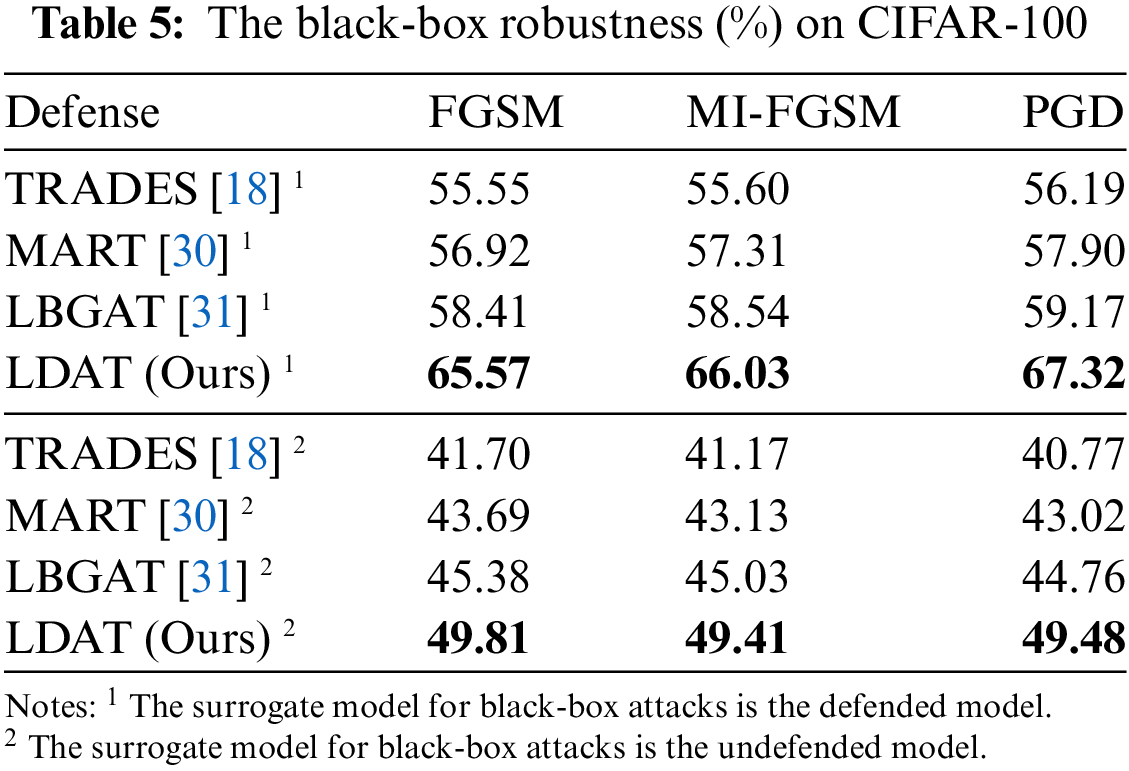
Three types of attack methods were chosen to target the surrogate model, evaluating black-box robustness in this paper. Two different surrogate models are used here: i) undefended: undefended model training with only natural examples on a more complicated model (for example, on CIFAR-10, the surrogate model is ResNet-50; on CIFAR-100, it is WideResNet-28-10), ii) defended: robust model through Madry’s method [14] on the model structure identical to the defense model. The surrogate and defense models were trained separately on the training set, without additional data and pre-trained models.

The natural accuracy of the natural training surrogate model on CIFAR-10 is 95.02%, and that of the natural training surrogate model on CIFAR-100 is 80.57%. The following attacks (FGSM [6], MI-FGSM [38], and PGD [14]) were employed to evaluate the black-box robustness under the L∞ threat model in this paper. The perturbation budget ϵ∞ is set to eight (out of 255) for all the datasets. These settings are the same as those for the white-box attack. MI-FGSM with 10 steps and a decay parameter of 1. PGD attacks for 40 steps with a step size of two (out of 255).

The black-box robustness of all defense models is presented in Tables 4 and 5. The proposed method outperforms the other baselines in terms of robustness. When the surrogate model is a natural training model, the robust accuracy of the model approaches that of natural images. When the surrogate model is defended, the adversarial examples exhibit significant transferability. This implies that the adversarial training model could serve as a surrogate model for black-box attacks, presenting a practical solution to significantly enhance the transferability of adversarial examples.

4.3 Impact of Perturbation Magnitude and Iteration Numbers on Model Robustness

Finally, the robustness of the model under various perturbation magnitudes and iterations of adversarial examples was analyzed. The PreAct ResNet-18 model on CIFAR-10 is subjected to an attack in this paper. For different perturbation magnitudes of adversarial examples, a PGD attack is used to investigate the robustness of the defense model. The number of iterations of PGD is set to 40. For different numbers of iterations of adversarial examples, the robust model is evaluated using the L∞ version of the PGD attack and the L2 version C&W attack. Under L∞ threat model, the perturbation magnitudes ϵ∞ = 8/255. Under L2 threat model, the perturbation magnitude ϵ2 = 0.5.

The robust accuracy of the defense model with different perturbation magnitudes is shown in Fig. 4. For small perturbation adversarial examples, LDAT does not exhibit many advantages under various threat models.

Figure 4: Robust accuracy (%) of defense models against PGD attacks on CIFAR-10. Under L∞-norm threat model, the TRADES curves overlap with those of MART and LBGAT

The robustness of all defense models showed a significant decrease as the magnitude of perturbation increased. However, the decrease in the robustness of LDAT is significantly less than that of the other defense methods, and there is a trend toward a slower rate of decrease. This indicates that the proposed method outperforms adversarial examples with large adversarial perturbations. This phenomenon is attributed to the collaboration of the proposed method with the model classification ability and sample distribution constraints.

The robust accuracy of the defense model for different iterations of adversarial attacks is shown in Fig. 5. It can be observed that LDAT can defend against multi-iteration attack methods. However, as the number of iterations increases, LDAT exhibits an obvious decrease in robustness, but still maintains its advantage over other defense methods.

Figure 5: The robust accuracy (%) of the defense models against PGD (L∞ threat model, ϵ∞ = 8/255) and C&W (L2 threat model, ϵ2 = 0.5) attack on CIFAR-10

4.4 Impact of Adversarial Attack Algorithm

LDAT boosts adversarial training by introducing a learnable distribution that can be learned from both natural and adversarial examples. It is difficult to learn the same distribution for natural and adversarial examples when adversarial examples cross over with natural examples. As shown in Fig. 6, the proposed attack algorithm is replaced with other common adversarial attack methods. When the cross-entropy and KL versions of the PGD attack are used to generate adversarial examples, the final robustness significantly decreases. This suggests that adversarial training using such attack methods does not consider that the decision boundary suffers from insufficient learning.

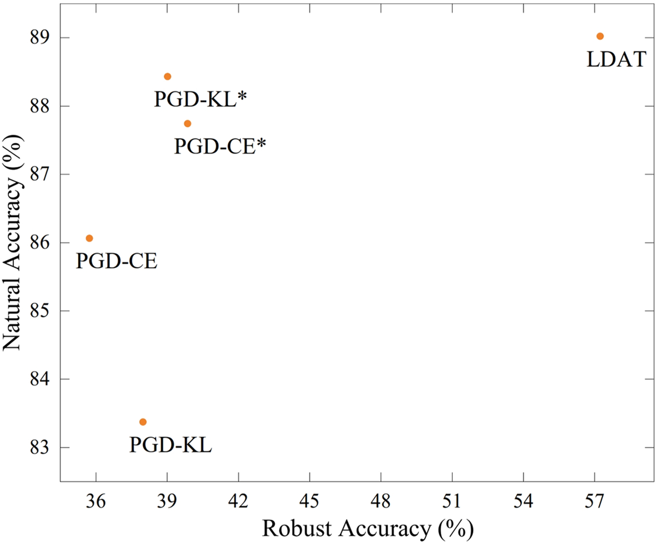
Figure 6: Replacing proposed attack algorithm with the variants of PGD attack, where * denotes the PGD of the L∞ version, and without * denotes the PGD of the L2 version

In this paper, the magnitude of the perturbation is scaled based on the decision boundary. This makes it as easy as possible for the model to learn natural and adversarial examples using the same distribution. Samples with stronger adversarial properties were added to the adversarial training process as the model robustness increased. Moreover, the adversarial example search range is wider than that of the PGD attack in the proposed algorithm because the perturbation is clipped only at the end of the iteration. These methods generate adversarial examples that are too strong, which prevents the model from learning the exact distribution centroid, thus hurting the model’s robustness.

4.5 Feature Visualization

The latent features of the samples on the test images of CIFAR-10 were visualized in this paper. Several natural examples and their corresponding adversarial examples are randomly sampled in each class. Feature visualization of the latent features extracted from TRADES (left) and LDAT (right) was performed by using t-SNE. Fig. 7 illustrates the well-clustered and separated latent features extracted by LDAT. The proposed method performed well for both natural and adversarial examples.

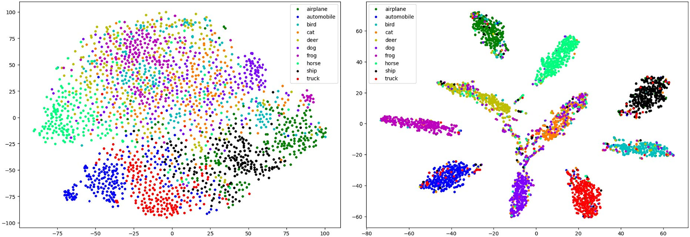
Figure 7: The t-SNE visualization of latent features extracted from TRADES (left) and LDAT (right) on the CIFAR-10 test set

The classification centroid learned from natural and adversarial examples can constrain the distribution, both of which benefit the defense model in classifying natural and adversarial examples. This leads to better robustness of LDAT than TRADES on attacks such as FGSM, PGD, and C&W.

4.6 Likelihood Distribution of Adversarial Examples

Instead of the fully connected layer, the Gaussian mixture model can not only perform classification, but also provide a likelihood estimation for the sample. Various types of adversarial examples have been shown to exhibit distribution differences in likelihood estimations. PGD, C&W, and FAB attacks were employed to generate adversarial examples on the CIFAR-10 test images in this paper. The likelihood of the samples is normalized using SoftMax loss for comparison. The histograms of the natural and adversarial examples are shown in Fig. 8.

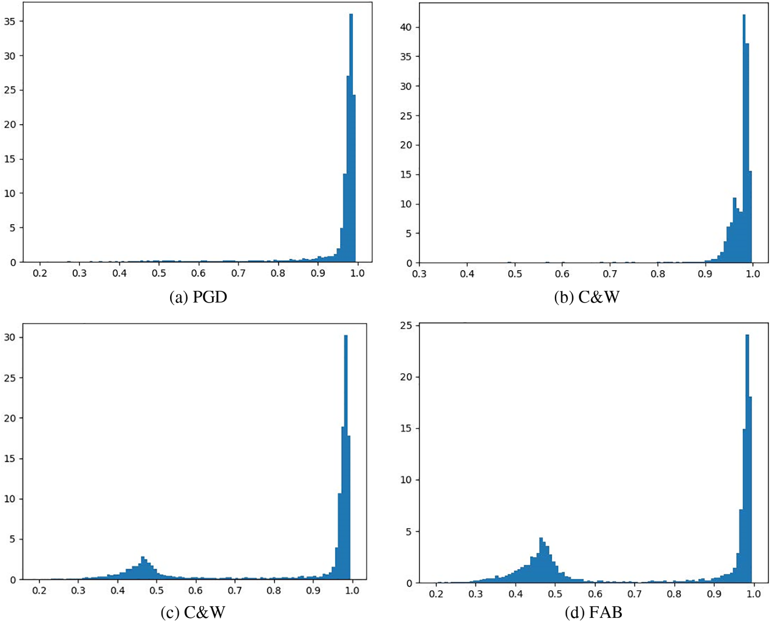
Figure 8: Likelihood estimation histograms for natural and adversarial examples. SoftMax was applied to the likelihood values of the model output to simplify visualization

It is observed that adversarial examples generated by PGD attacks and natural examples are classified with high confidence. This is consistent with the discovery of Zhang et al. [24], where extremely strong adversarial examples were mixed with the corresponding natural examples. This mixture phenomenon makes adversarial training difficult, and makes it difficult to distinguish natural examples from adversarial examples in terms of likelihood estimation.

Moreover, some interesting phenomena of adversarial examples generated by specific attack methods in the proposed method were observed. For some adversarial attacks, such as C&W (k = 0) and FAB, both high-confidence and low-confidence adversarial examples exist among the adversarial examples generated by these methods. According to the analysis of the above adversarial examples, the adversarial examples that can be successfully attacked tend to have low confidence. This means that the model can reject classification for low-confidence examples to defend against adversarial attacks. A threshold value (e.g., 0.6) is set for detecting adversarial examples, which has almost no effect on natural examples.

The defense success rate used to measure the robustness of the model, which is defined as the combination of detection and classification accuracy. The detection accuracy indicated that the misclassified samples in the test data were rejected. The classification accuracy represents the rate of correctly classified samples in the test data after detection. The defense success rates of natural and adversarial examples are shown in Fig. 9.

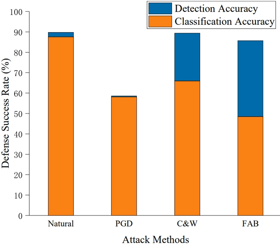
Figure 9: Defense success rates of natural and adversarial examples. The defense success rate is the sum of the detection and the classification accuracy

For high-confidence adversarial examples, the threshold is not needed to improve the defense success rate. However, for low-confidence adversarial examples, the samples that triggered misclassification can be detected easily. This indicates that the proposed method is robust to the model while providing the model with the ability to detect partial adversarial examples.

5  Conclusion

In this paper, a novel adversarial training method is proposed, aiming to close the distribution gap between natural and adversarial examples. In contrast to the existing adversarial defense methods, the proposed method enables both natural and adversarial examples to follow the same distribution. Moreover, an adversarial attack algorithm for adversarial training was proposed based on the decision boundary of the model in this paper. The proposed adversarial attack can gradually increase the perturbation budget and help the model learn the robustness distribution centroid. Finally, comprehensive experiments showed that adversarial-trained models using the proposed method performed well in terms of both accuracy and robustness.

In the future, the adversarial attack algorithm will be further improved to obtain a more robust classification centroid. In addition, more exploration on the possibility of improving model robustness by exploiting the likelihood estimation of model output.

Acknowledgement: We the authors, would like to express our sincere gratitude and appreciation to each other for our combined efforts and contributions throughout the course of this research paper.

Funding Statement: This work was supported by the National Natural Science Foundation of China (No. U21B2003, 62072250, 62072250, 62172435, U1804263, U20B2065, 61872203, 71802110, 61802212), and the National Key R&D Program of China (No. 2021QY0700), and the Key Laboratory of Intelligent Support Technology for Complex Environments (Nanjing University of Information Science and Technology), Ministry of Education, and the Natural Science Foundation of Jiangsu Province (No. BK20200750), and Open Foundation of Henan Key Laboratory of Cyberspace Situation Awareness (No. HNTS2022002), and Post Graduate Research & Practice Innvoation Program of Jiangsu Province (No. KYCX200974), and Open Project Fund of Shandong Provincial Key Laboratory of Computer Network (No. SDKLCN-2022-05), and the Priority Academic Program Development of Jiangsu Higher Education Institutions (PAPD) Fund and Graduate Student Scientific Research Innovation Projects of Jiangsu Province (No. KYCX231359).

Author Contributions: The authors confirm contribution to the paper as follows: study conception and design: K. Chen, J Wang; analysis and interpretation of results: K. Chen, Y. Dai; draft manuscript preparation: J. M. Adeke, G Liu. All authors reviewed the results and approved the final version of the manuscript.

Availability of Data and Materials: The datasets analyzed during the current study are available in the Science Data Bank repository, https://www.scidb.cn/en/detail?dataSetId=Z_582892.

Conflicts of Interest: The authors declare that they have no known competing financial interests or personal relationships that could have appeared to influence the work reported in this paper.

References

1. H. Yoo, S. Lee, and K. Chung, “Deep learning-based action classification using one-shot object detection,” Comput. Mater. Contin., vol. 76, no. 2, pp. 1343–1359, 2023. doi: 10.32604/cmc.2023.039263. [Google Scholar] [PubMed] [CrossRef]

2. Q. Arshad et al., “Anomalous situations recognition in surveillance images using deep learning,” Comput. Mater. Contin., vol. 76, no. 1, pp. 1103–1125, 2023. doi: 10.32604/cmc.2023.039752. [Google Scholar] [PubMed] [CrossRef]

3. Z. Weng, Z. Qin, X. Tao, C. Pan, G. Liu and G. Y. Li, “Deep learning enabled semantic communications with speech recognition and synthesis,” IEEE Trans. Wirel. Commun., vol. 22, no. 9, pp. 6227–6240, 2023. doi: 10.1109/TWC.2023.3240969. [Google Scholar] [CrossRef]

4. Y. Yang, Y. Liu, T. Bao, W. Wang, N. Niu and Y. Yin, “DeepOCL: A deep natural network for object constraint language generation from unrestricted nature language,” CAAI Trans. Intell. Technol., vol. 22, no. 9, pp. 6227–6240, 2023. doi: 10.1049/cit2.12207. [Google Scholar] [CrossRef]

5. J. K. Devlin, M. W. Chang, and L. K. Toutanova, “BERT: Pre-training of deep bidirectional transformers for language understanding,” arXiv preprint arXiv:1810.04805, 2018. [Google Scholar]

6. I. J. Goodfellow, J. Shlens, and C. Szegedy, “Explaining and harnessing adversarial examples,” arXiv preprint arXiv:1412.6572, 2014. [Google Scholar]

7. H. Hirano, A. Minagi, and K. Takemoto, “Universal adversarial attacks on deep neural networks for medical image classification,” BMC Med. Imaging, vol. 21, pp. 1–13, 2021. doi: 10.1186/s12880-020-00530-y. [Google Scholar] [PubMed] [CrossRef]

8. A. M. Roy, J. Bhaduri, T. Kumar, and K. Raj, “WilDect-YOLO: An efficient and robust computer vision-based accurate object localization model for automated endangered wildlife detection,” Ecol. Inform., vol. 75, pp. 101919, 2023. doi: 10.1016/j.ecoinf.2022.101919. [Google Scholar] [CrossRef]

9. H. Wei, Q. Zhang, Y. Qian, Z. Xu, and J. Han, “MTSDet: Multi-scale traffic sign detection with attention and path aggregation,” Appl. Intell., vol. 53, no. 1, pp. 238–250, 2023. doi: 10.1007/s10489-022-03459-7. [Google Scholar] [CrossRef]

10. H. Wen, S. Chang, and L. Zhou, “Light projection-based physical-world vanishing attack against car detection,” in ICASSP 2023–2023 IEEE Int. Conf. Acoust, Speech Signal Process (ICASSP), Rhodes Island, Greece, 2023, pp. 1–5. [Google Scholar]

11. J. Wu, J. Wang, J. Zhao, X. Luo, and B. Ma, “ESGAN for generating high-quality enhanced samples,” Multimed. Syst., vol. 28, no. 5, pp. 1809–1822, 2022. doi: 10.1007/s00530-022-00953-3. [Google Scholar] [CrossRef]

12. S. Jung, M. Chung, and Y. Shin, “Adversarial example detection by predicting adversarial noise in the frequency domain,” Multimed. Tools Appl., vol. 82, no. 16, pp. 25235–25251, 2023. doi: 10.1007/s11042-023-14608-6. [Google Scholar] [CrossRef]

13. T. Dai, Y. Feng, B. Chen, J. Lu, and S. T. Xia, “Deep image prior-based defense against adversarial examples,” Pattern Recognit., vol. 122, pp. 108249, 2022. doi: 10.1016/j.patcog.2021.108249. [Google Scholar] [CrossRef]

14. A. Madry, A. Makelov, L. Schmidt, D. Tsipras, and A. Vladu, “Towards deep learning models resistant to adversarial attacks,” arXiv preprint arXiv:1706.06083, 2017. [Google Scholar]

15. A. Shafahi et al., “Adversarial training for free!” in Adv. Neural Inf. Process Syst., Vancouver, Canada, vol. 32, 2019. [Google Scholar]

16. F. Tramèr, A. Kurakin, N. Papernot, I. Goodfellow, D. Boneh and P. McDaniel, “Ensemble adversarial training: Attacks and defenses,” arXiv preprint arXiv:1705.07204, 2017. [Google Scholar]

17. F. Xu, Y. Bao, B. Li, Z. Hou, and L. Wang, “Entropy minimization and domain adversarial training guided by label distribution similarity for domain adaptation,” Multimedia Syst., vol. 29, no. 4, pp. 2281–2292, 2023. doi: 10.1007/s00530-023-01106-w. [Google Scholar] [CrossRef]

18. H. Zhang, Y. Yu, J. Jiao, E. Xing, L. El Ghaoui and M. Jordan, “Theoretically principled trade-off between robustness and accuracy,” in Int. Conf. Mach. Learn., Long Beach, USA, vol. 97, 2019, pp. 7472–7482. [Google Scholar]

19. H. Kannan, A. Kurakin, and I. Goodfellow, “Adversarial logit pairing,” arXiv preprint arXiv:1803.06373, 2018. [Google Scholar]

20. C. Xie and A. Yuille, “Intriguing properties of adversarial training at scale,” arXiv preprint arXiv:1906.03787, 2019. [Google Scholar]

21. C. Xie, M. Tan, B. Gong, J. Wang, A. L. Yuille and Q. V. Le, “Adversarial examples improve image recognition,” in Proc. IEEE/CVF Conf. Comput. Vis. Pattern Recognit., Seattle, USA, 2020, pp. 819–828. [Google Scholar]

22. N. Carlini and D. Wagner, “Towards evaluating the robustness of neural networks,” in 2017 IEEE Symp. Secur. Priv. (SP), San Jose, USA, 2017, pp. 39–57. [Google Scholar]

23. Q. Z. Cai, M. Du, C. Liu, and D. Song, “Curriculum adversarial training,” arXiv preprint arXiv:1805.04807, 2018. [Google Scholar]

24. J. Zhang et al., “Attacks which do not kill training make adversarial learning stronger,” in Int. Conf. Mach. Learn., Vienna, Austria, 2020, pp. 11278–11287. [Google Scholar]

25. Y. Wang, X. Ma, J. Bailey, J. Yi, B. Zhou and Q. Gu, “On the convergence and robustness of adversarial training,” arXiv preprint arXiv:2112.08304, 2021. [Google Scholar]

26. A. Kurakin, I. Goodfellow, and S. Bengio, “Adversarial machine learning at scale,” arXiv preprint arXiv:1611.01236, 2016. [Google Scholar]

27. A. Krizhevsky and G. Hinton, “Learning multiple layers of features from tiny images,” Technical Report, University of Toronto, Canada, 2009. [Google Scholar]

28. K. He, X. Zhang, S. Ren, and J. Sun, “Identity mappings in deep residual networks,” in Comput. Vis–ECCV 2016: 14th Eur. Conf., Amsterdam, The Netherlands, 2016, pp. 630–645. [Google Scholar]

29. S. Zagoruyko and N. Komodakis, “Wide residual networks,” arXiv preprint arXiv:1605.07146, 2016. [Google Scholar]

30. Y. Wang, D. Zou, J. Yi, J. Bailey, X. Ma and Q. Gu, “Improving adversarial robustness requires revisiting misclassified examples,” in Int. Conf. on Learning Representations, Ethiopia, Millennium Hall, Addis Ababa, 2020. [Google Scholar]

31. J. Cui, S. Liu, L. Wang, and J. Jia, “Learnable boundary guided adversarial training,” in Proc. IEEE/CVF Int. Conf. Comput Vis., 2021, pp. 15721–15730. [Google Scholar]

32. J. Rauber, W. Brendel, and M. Bethge, “Foolbox: A python toolbox to benchmark the robustness of machine learning models,” arXiv preprint arXiv:1707.04131, 2017. [Google Scholar]

33. H. Kim, “Torchattacks: A pytorch repository for adversarial attacks,” arXiv preprint arXiv:2010.01950, 2020. [Google Scholar]

34. F. Croce and M. Hein, “Reliable evaluation of adversarial robustness with an ensemble of diverse parameter-free attacks,” in Int. Conf. Mach. Learn., Austria, Vienna, 2020, pp. 2206–2216. [Google Scholar]

35. F. Croce and M. Hein, “Minimally distorted adversarial examples with a fast adaptive boundary attack,” in Int. Conf. Mach. Learn., Austria, Vienna, 2020, pp. 2196–2205. [Google Scholar]

36. S. M. Moosavi-Dezfooli, A. Fawzi, and P. Frossard, “Deepfool: A simple and accurate method to fool deep neural networks,” in Proc. IEEE Conf. Comput. Vis. Pattern Recognit., Las Vegas, USA, 2016, pp. 2574–2582. [Google Scholar]

37. J. Rony, L. G. Hafemann, L. S. Oliveira, I. B. Ayed, R. Sabourin and E. Granger, “Decoupling direction and norm for efficient gradient-based L2 adversarial attacks and defenses,” in Proc. IEEE/CVF Conf. Comput. Vis. Pattern Recognit., Long Beach, USA, 2019, pp. 4322–4330. [Google Scholar]

38. Y. Dong et al., “Boosting adversarial attacks with momentum,” in Proc. IEEE Conf. Comput. Vis. Pattern Recognit, Salt Lake City, USA, 2018, pp. 9185–9193. [Google Scholar]