Unsupervised Color Segmentation with Reconstructed Spatial Weighted Gaussian Mixture Model and Random Color Histogram

1  Introduction

Image segmentation is the process of decomposing a digital image into several regions having similar characteristics to obtain a significant form of the image [1,2]. Segmentation [3–5] plays a central role in a broad range of applications [6–8]. It is a commonly used critical step in many image understanding algorithms [9,10], practical computer vision systems [11,12], and object recognition [13–15]. Moreover, the fundamental objective of image segmentation is to depict an image using a limited number of meaningful segments rather than an excessive number of individual pixels. Additionally, the concept of image segmentation can be viewed as a clustering methodology, wherein pixels that meet a specific criterion are organized into a cluster, while pixels that lack the requirement are assigned to separate groups.

Recently, various methods, such as boundary-based image segmentation [16,17] have been introduced for image segmentation [18]. Boundary-based algorithms search for the most dissimilar pixels. The dissimilarity, which represents discontinuities in the image, can be processed via segmentation and pixel labeling. Region-based methods [19] search for the most similar areas. On the contrary, color histogram methods are strongly based on pixel colors to describe for each color level the number of corresponding pixels which usually convert images in color space such as RGB, or HSV. The algorithms [20] incorporate pixel-based clusters depending on their intensity and spatial locations.

In computer vision, image segmentation is the prime research area which is equivalent to dividing an image into its objects or regions of interest. It groups the image pixels into sections that are similar to each other. Numerous image-based applications, including pattern recognition, biometric identification, medical imaging, object detection and classification, and pre-processing, go through this stage [21]. Several notable uses include content-based image retrieval [21–23], machine vision [24,25], medical image analysis [26,27], object recognition [28], and autonomous vehicle video surveillance [29]. Content-based image retrieval [30] is the process of searching for digital images that are relevant to a given query within extensive databases. The retrieval results are acquired based on the content of the query image. Image segmentation is employed to extract the contents contained inside an image. Machine vision [31] utilizes image-based technologies for robotic inspection and analysis, primarily within industrial settings. Segmentation is a procedure that involves extracting relevant information from a collected image that is associated with a machine or processed information. Medical imaging [32] plays a crucial role in various aspects of medical science, encompassing medical diagnosis and treatments [33]. Image segmentation, in particular, has emerged as a valuable tool in this domain, facilitating the analysis and interpretation of medical images. Several instances may be cited to illustrate the application of image segmentation in medical imaging. One such example is the segmentation of tumors, which is performed to accurately locate their presence within the body. Additionally, the segmentation of tissue is employed to measure the corresponding volumes of specific anatomical structures. Furthermore, the segmentation of cells is utilized to facilitate numerous digital pathological activities. Various parameters can be included in the analysis of cellular characteristics, such as cell count and nuclei categorization, among others. Object recognition and detection [34,35] is a significant application within the field of computer vision. In this context, an object may be denoted as a pedestrian, a facial structure, or various aerial entities such as highways, forests, crops, and so on. This application is crucial for the process of image segmentation, as it facilitates the extraction of the intended item from the image. Video surveillance [36] involves the utilization of video cameras to record and monitor the movements inside a certain area of interest. These recorded videos are then analyzed to accomplish specific objectives, such as identifying the actions taking place in the footage or managing the flow of traffic. Quantifying the quantity of things and various other tasks. In order to do the analysis, segmentation is required. A thorough understanding of the region under investigation is of paramount importance.

Although humans may perceive the task of segmenting an image into its relevant segments as straightforward, it is rather challenging for computer vision systems. There exist a multitude of issues that have the potential to impact the performance of an image segmentation method. A variation in illumination is a key issue endured in the process of image segmentation, which has major effects on distinct pixels. The observed variation is driven by the diverse lighting conditions present during the process of image capture. Intra-class variation is an immense obstacle in this domain since it entails the presence of diverse manifestations or formations of the region of interest. The complexity of the backdrop is the presence of a complicated background in an image poses a significant obstacle. The process of segmenting an image into regions of interest can be challenging due to the presence of complex environmental factors and various limitations.

While there are various challenges and limitations to unsupervised image segmentation, the field of image segmentation in artificial intelligence research is undergoing significant development, employing sophisticated methodologies to detect and separate individual components within an image without the need for human guidance. The proposed unsupervised object segmentation methodology frequently entails spatial insertion, wherein the algorithm discerns the precise positioning of objects within a designated spatial domain. A noteworthy approach involves the incorporation of saliency residuals, a technique that emphasizes regions within a picture that exhibit distinctiveness in comparison to their surrounding context. This method proves beneficial in facilitating the process of object detection. The aforementioned proposed technique is frequently used with Gaussian mixture models (GMM), a statistical technique that characterizes the existence of subpopulations within a larger population. In the context of this scenario, Gaussian mixture models are employed to analyze individual pixels or clusters of pixels in a picture. This process facilitates the grouping of comparable regions, hence assisting in the differentiation of separate entities. In conclusion, the utilization of random color histograms is employed as a technique to examine the dispersion of colors inside an image, introducing an additional level of distinction for various items. The complex nature of this approach is indicative of the convergence of multiple research fields, such as statistics, computer vision, and cognitive science, each offering distinct perspectives and methodologies. Interdisciplinary contributions can be observed in various domains, such as neurology, where knowledge of human perception informs the design of algorithms, or in data analytics, where clustering techniques guide approaches for image segmentation. The amalgamation of these disparate disciplines highlights the comprehensive character of progress in artificial intelligence, wherein the incorporation of separate ideas and approaches yields more resilient and efficient solutions.

1.1 Supervised & Unsupervised Categories

Image segmentation can be classified into two categories: supervised segmentation and unsupervised segmentation. The supervised classification primarily employs convolutional neural network (CNN) and fully convolutional network (FCN) methodologies for image segmentation. These techniques are feature-based learning approaches, performed to label the images and detect the object of interest with the aid of human guidance. Supervised segmentation requires special train data for residual region detection. For instance, Benediktsson et al. [37] obtained the basic features using morphological characterizations and analyzed these features using neural networks. Most deep learning methods require a large amount of manually labeled data restricted to different scenarios. These methods are highly expensive for large-scale image classification. However, unsupervised methods are effective and popular owing to their simplicity as well as their ability to work without training data and labeling images. This category instantly detects and distinguishes the residual region, including the edge density feature [13], using local feature points [38,39] without training data. An unsupervised segmentation approach attempts to automate the determination of the number of resultant regions in the image and allocates optimal parameter values for the segmentation algorithm [40]. Various unsupervised segmentation algorithms employ clustering techniques such as C-means clustering [1,2], Gaussian mixture model [41,42], K-means clustering [43], graph cut [44], and so on for image segmentation. These color segmentation techniques, which depend on the color feature of image pixels, assume that similar colors in the image correspond to separate clusters, and hence meaningful objects in the image. Each cluster defines a pixel class that shares similar color properties. Since the segmentation results depend on the color space, a single-color space cannot yield satisfactory results for all types of images. Therefore, several researchers have tried to determine the color space that corresponds to the color image segmentation problem being studied [45,46]. A color space can be defined as a systematic arrangement or structure that categorizes and organizes colors. In addition to the process of physical device profiling, color spaces play a crucial role in facilitating the accurate reproduction of color in both analog and digital formats. Color spaces can be conceptualized as a theoretical mathematical framework that facilitates the numerical representation of colors. Color theory is an academic discipline that elucidates the mechanisms underlying human perception of color. This perceptual phenomenon arises from the interplay between the absorption, reflection, and transmission of light by the surrounding objects. When an object is illuminated by light, certain wavelengths are assimilated while others are reflected. It is through this process of reflection that we can see the color of the thing. However, it is important to note that individuals possess diverse cultural and environmental associations with color, which therefore influence our perceptions. In this work, we combine the hue, saturation, value (HSV) model and the CIELUE color space with the residual approach for the extraction of color saliency, to maximize the accuracy of the segmentation process.

1.2 Related Clustering Approach

Clustering association rules and the organization of common features of clusters are in general critical problems encountered in various domains of science. Image segmentation can be considered as a specific type of clustering. Clustering-based algorithms are widely used for segmentation owing to their fast and efficient operation. Clustering aims to partition a set of data into clusters such that similar data sets are grouped in the same clusters, and dissimilar data sets are grouped in different clusters [1]. The purpose of clustering is to group data points into classes entirely without labels [47]. In unsupervised segmentation models, the clustering algorithm is widely used for grayscale and color segmentation, which is beneficial for low- and high-dimensional data. Several model-based clustering techniques have been presented to address the challenge of unsupervised image segmentation. Such as, Gauss-Markov random fields [48,49] utilize the property that the conditional distribution of each data point given all other points is Gaussian. The model is characterized by its local dependencies and is commonly employed in the field of spatial data analysis. Gibbs random fields [50] are the specific instances of Markov random fields observed, wherein the collective distribution of all data points is represented as a multiplication of potential functions, with each function contingent upon a subset of data points [51]. Gaussian autoregressive random fields [52] are characterized by the property that the value of a variable is determined as a linear combination of the values of its neighboring variables, along with a Gaussian noise term. Time series and geographical analysis frequently employ this methodology. In univariate and multivariate analyses [53] in the context of clustering, the term feature-wise pertains to the methodology wherein each feature is examined independently. The approach is straightforward, although it fails to account for any potential relationships among the features. The multivariate approach [54] under consideration concurrently takes into account various variables and is capable of accounting for relationships among the features. The concept of data clusters is characterized by its complexity, however, it offers a comprehensive perspective on the subject matter. In the Gaussian density model, it is assumed that the data is derived from an unimodal Gaussian distribution. The proposed model is characterized by its simplicity and effectiveness in cases when the data exhibit a natural tendency to form a cohesive group. The Gaussian mixture model [55] is an extension of the Gaussian density model, which posits that the observed data is formed from a mixture of many Gaussian distributions. The flexibility of the system allows for the modeling of intricate data structures. The clustering processing has distinct features that spatial should be driven into description. For example, an image segmentation clustering process specifies local features in the description. This means that in addition to density values, pixel neighbors are predominantly used to assign each pixel to a specific cluster. In most images, the cluster label is intentionally allowed to scatter between adjacent spatial pixels. The incorporation of randomness in models like Gauss-Markov random fields, Gibbs random fields, Markov random fields, Gaussian autoregressive random fields, and Gaussian mixture models is fundamental for capturing the inherent complexities and uncertainties of data, particularly in spatial and statistical analysis. In summary, randomness in these models is crucial for accounting for the inherent uncertainties and variabilities in real-world data, enabling them to be more adaptable, flexible, and capable of capturing complex data structures and relationships.

Recently, Balasubramanian et al. [56] proposed a hybrid approach that combines the gradient method with Otsu’s method for unsupervised image segmentation. Bosch et al. [57] exploited the diversity of segments produced by different choices of parameters and generated hypotheses to under-segment an image. Kanezaki [58] joined pixels of similar features and assigned unique labels to spatially continuous pixels during the self-training process, which enabled unsupervised image segmentation. The local spatial information is incorporated into the fast robust fuzzy c-means [1] and the super pixel fast fuzzy c-means [2] algorithms to enhance the segmentation effect. The automatic fuzzy clustering framework based on prior entropy [59] incorporates spatial information. The proposed approaches demonstrate interesting performances. Among these approaches, the main focus is on the GMM for unsupervised image segmentation. The GMM is a well-known mechanism utilized for image segmentation [60,61] and object segmentation in a video [62–64]. The expectation-maximization (EM) [65–68] method is usually used to evaluate the parameters of the distribution. However, similar to measurable mixture models, GMM does not analyze spatial information in images. The traditional GMM estimates each pixel independently, but the objects of interest in the image constitute relevant pixels that assign some shared statistical features such as values, colors, textures, and so on. Several approaches that incorporate spatial information have been introduced to enhance traditional GMM [69,70]. The Markov random field (MRF) [71] was used for supervising neighboring pixel dependencies and measuring the level of smoothness for each cluster. Therefore, it was recommended that spatial characteristics be included in the MRF-constructed mixture model [70,71] for image segmentation. The main drawbacks of these models are complicated parameter estimation and the high computational complexity of the MRF model. The mixture model [72,73], a pixel labeling algorithm based on GMM, assigns pixels, and each pixel represents a distinct segment for the probability distribution. Parameter estimation can be achieved efficiently using the maximum likelihood (ML) method and the expectation-maximization (EM) algorithm. After parameter estimation, the ML and EM assign a maximum posteriori (MAP) estimate to each pixel. However, the computational cost reduces their effective utilization in functional applications. Reference [74] included local spatial information by implementing a mean template, and it has been extended to [75,76] either arithmetic or weighted. Despite the fact, that these models had high execution speeds, were robust to noise, and uniformly allocated weights to the neighbor pixels. Additionally, obtaining precise segmentation in color images is extremely challenging and complicated. Achieving satisfactory segmentation depends essentially on methods for identifying similarities amongst feature values of images and appropriate established regions that display similarities. Hence, there is a demand to integrate color saliency as spatial information into the GMM process, which produces remarkable results in overcoming the drawbacks of the GMM process and offers nature segmentation results. The proposed method introduces color saliency as spatial information using a neighborhood-weighted GMM distribution process. The original RGB image is transformed into HSV to extract the salient residual region. The resultant color saliency is constructed via pixel multiplication of the residual features of the salient region with the spatial features of CIE-LUV color. In the second stage, the color saliency is incorporated as spatial information in the GMM to obtain a desirable histogram of a particular sub-band of the color image. The EM method returns an average corresponding to a cluster and uses the return index to label the particular cluster of the image. The pixel-cluster association by multiplication with the color saliency highlights the significant region. In the final step, the implemented random color histogram assigns a unique color to each cluster, which quickly yields significantly accurate segmentation results. These highlights have advanced the significance of the proposed model in conventional real-world applications. Fig. 1 depicts successful implementation of the proposed model. This proposal is novel in that it incorporates color saliency as spatial information in GMM using a random color histogram for unsupervised image segmentation.

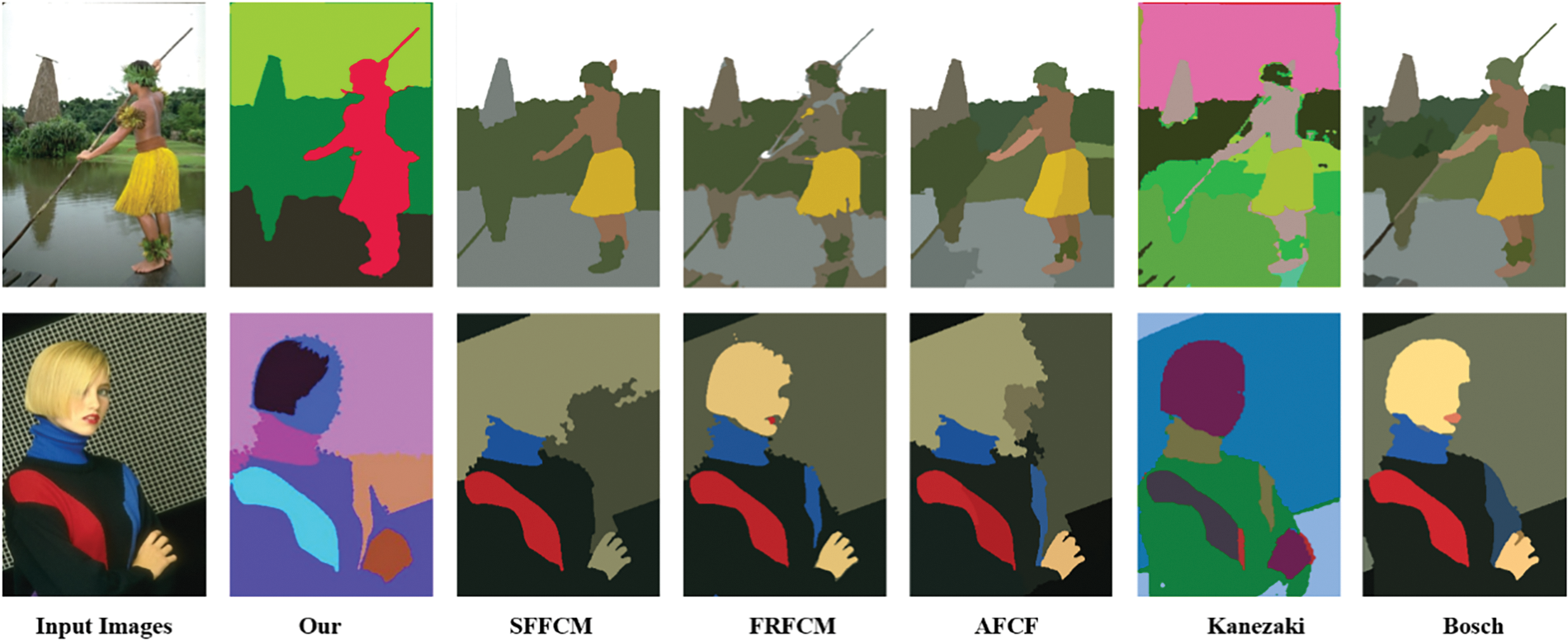
Figure 1: In this visual illustration, we meticulously assess the efficacy of several leading-edge models in the realm of object segmentation. This includes an exploration of the SFFCM, FRFCM, and AFCF algorithms. Furthermore, we delve into the nuances of Kanezaki and Bosch model, alongside our innovatively proposed algorithm. The visual outcomes compellingly demonstrate that our method achieves exceptional accuracy in object segmentation when contrasted with the other algorithms

In this study, we propose an unsupervised image segmentation model that produces high-quality segmentation results with low computational cost, yet achieves a high segmentation accuracy. This study can be summarized as follows:

1.    The prior feature and texture estimation are extracted by transforming the image to the HSV and CIE-LUV [77] color space. These features allow the detection and construction of color saliency during image processing.

2.    The color saliency is incorporated as spatial information in the GMM. The spatial information highlights the role of meaningful pixels in assigning some specific weight to neighbor pixels of the current pixels.

3.    The expectation maximization (EM) algorithm of the Gaussian mixture model better controls the range of the color and removes turbidites.

4.    The general formwork of a random color histogram assigns a unique color to each unlabeled cluster as well as searches for the immediate (nearest neighbor) label end implemented for enhancing segmentation results.

The implementation of the traditional clustering approach is complicated and results in poor image segmentation. GMM is suitable for hard clustering, sensitive to ambiguity, and preserves additional innovative image information. The proposed model incorporating color saliency as a spatial information in GMM successfully supports the preliminary aim of the proposed model for unsupervised image segmentation. GMM is free from any parameter selection and is robust to images corrupted by noise. GMM segments images with complex backgrounds in an efficient and significantly effective manner. The incorporation of spatial information and implementation of the random color histogram in the final stage strengthen and enhance the unsupervised segmentation process. Further advantages offered by our proposed algorithm are mentioned below:

1.    The proposed algorithm offers an automatic clustering framework and operates effectively without parameters.

2.    The utilization of the random color histogram and the spatial information inside GMM provides accurate segmentation compared to other state-of-the-art algorithms.

3.    The spatial information in the form of color saliency is used as a penalty term, which minimizes the overall computational cost in segmentation processing.

The remainder of the paper is organized as follows: Section 2 describes the probabilistic model for image segmentation and presents the improvements made to the proposed model; Section 3 provides the comparative experimental results and tradeoff; and finally, Section 4 presents the conclusions and future scope.

2  The Proposed Method

The three steps involved in developing the proposed statistical model for image segmentation are visually depicted in Fig. 2, and described as follows: first, the color saliency must be constructed; second, the color saliency must be included as spatial information in the GMM. The GMM estimates the mixture parameters and determines the number of Gaussian components. The GMM implements the EM algorithm to assign each pixel to an appropriate cluster, according to ML. Finally, the random color histogram is used to ensure accurate unsupervised image segmentation.

Figure 2: This illustration elegantly delineates the proposed spatial weighted Gaussian mixture model, designed for unsupervised image segmentation. It artfully unfolds the architecture, encompassing color transformation, salience residual, color saliency, the spatial weighted Gaussian mixture model itself, and a random color histogram, all seamlessly integrated for refining unsupervised image segmentation

2.1 The Salient Residual Color Saliency

The spectral residual model [78] is modified to extract color residential regions for constructing color saliency. The main steps involved in this process are described below. First, the original image is transformed into the HSV color [79,80] and CIE-LUV [81,82] color space to obtain spatial features. Next, the spectral model is applied to the HSV image to extract salient residual regions. Finally, color saliency is constructed by joint pixel multiplication of the spatial features of the CIE-LUV color space with the residual features of the salient region. The model drives to separate salient regions for further unsupervised image segmentation.

2.1.1 Color Transformation

The RGB color model is the color model that is generally accepted for representing image pixels. Usually, in color image processing, the intensity of a pixel is shown as three values corresponding to the tri-stimuli R (red), G (green), and B (blue). Various sets of color models, such as intensity, saturation, and LAB, can be derived from the RGB color model by utilizing either linear or non-linear conversions. Several color models such as CIE-LAB, CIE-LUV, and CIE XYZ, etc., are employed in various applications to determine complex problems in color image processing. The HSV color space, which can be easily adjusted, is further suitable for color extraction and can be easily inverted. In color clustering methods, the chosen color highlights should specify a consistent color space. Several well-organized research [17] on region segmentation have demonstrated that feature segments of the CIE color space are efficient mechanisms for solving the segmentation problem. In this approach, the RGB image is converted to HSV.

The HSV color space can be transformed into other shades. Additionally, we chose to represent a 3-channel RGB color image in terms of the L∗U∗V∗ color metric, which was specially designed to ensure the best approximation of perceptually uniform color spaces. The perceptually uniform CIE-LUV color values are also used as a color feature in our proposed method. The color and texture features improve the performance and facilitate the segmentation process. The current model implements the HSV and CIE-LUV color values, which are suitable for describing the texture feature distributions. Given an input image I(x), the HSV [68] and L∗U∗V∗ color space [81,83,84] random transformations can be written as:

IHSV(x→)=(xH,xS,xV)T.(1)

where xH represents Hue, xS represents Saturation, and xV represents value in the HSV color space.

ILUV(x→)=(XL∗,Xu∗,Xv∗)T.(2)

where XL∗ represents Luminance, Xu∗, and Xv∗ represent the chromaticity coordinates in the LUV color space.

The segmentation method commonly entails translating the image into the selected color space, doing random transformations, and subsequently segmenting the image by the utilization of clustering techniques such as the Gaussian mixture model. Achieving optimal results in this approach necessitates finding a suitable equilibrium between the extent of transformation and the quality of segmentation. This entails taking into account many elements such as computing complexity and the careful selection of relevant parameters. This post-processing approach is commonly employed to enhance and improve the outcomes of segmentation. The primary objective is to optimize segment discrimination while upholding the standards of precision and efficiency in the segmentation procedure.

2.1.2 Color Saliency Transformation

Hou et al. [78] analyzed the log spectra for a large number of original images and observed that the log spectra of complex images share similar trends. Hence, the details of the plane curves must be displayed in various log spectra, which are significantly similar in shape. It is assumed that the statistical characteristics of color may be effective for irregular objects and regions in the image, where features of the objects are displayed. On subsequent investigation, the spectral residential model is observed to drive the salient residual region from transformed spectral residuals. Therefore, the saliency map is computed according to [78,85].

We obtain frequency in the image f by f=F(IHSV(x→)), where F describes the Fourier Transformation. The amplitude spectrum and phase spectrum can be represented as A(f) and P(f), respectively, and expressed as shown below:

A(f)=abs(f),(3)

P(f)=angle(f).(4)

The spectral residual of the input image is defined as:

R(f)=L(f)−h(f)×L(f)(5)

where L(f) computed as L(f)=log(A(f)) is the log amplitude spectrum, h(f)×L(f) is the average log amplitude spectrum, which denotes the general shape of log spectra, and h(f) is a 3 × 3 local average filter defined by:

h(f)=13×3(111111111).(6)

Additionally, R(f) represents the residual regions. The saliency map in the spatial domain is constructed via inverse Fourier transform.

S(xs)=F−1[exp(R(f)+P(f))]2,(7)

The saliency measure is utilized on the HSV color image to generate a salient residual representation, which is denoted as Isaliency, where F−1 denotes the inverse Fourier transform. Finally, the color saliency is constructed using the joint formulation:

S(p)=F−1[exp(R(HSV(p))+P(HSV(p)))]2(8)

The formula for converting the original image I into a salient residual image saliency in the HSV color space can be expressed as follows:

Isaliency(p)=F−1[exp(R(HSV (p))+P(HSV (p)))]2∀p∈I(9)

2.2 Spatial Weighted Gaussian Mixture Model

Incorporating both spatial information [69,70] and color saliency into a GMM for image processing using the expectation-maximization (EM) algorithm is a technique to improve segmentation or clustering by considering both the color attributes and spatial relationships of pixels. Assuming we have the following definitions. Let M={m1,m2,…,mN} denotes the observed data where each mi is a pixel value in the image, C= {c1,c2,…,cN} represents the color saliency values corresponding to each pixel, U={uij} symbolize the spatial weights between pixels i and j, where these weights express the spatial relationship or proximity, Q={q1,q2,…,qN} signifies the latent variables indicating the component each pixel belongs to, φ={ξη,αη,Ση} forη=1,…,K represents the parameters of the GMM (mixing coefficients, means, and covariances, respectively). The goal of the spatial weighted GMM with color saliency is to cluster pixels not only based on their color (as in a standard GMM) but also considering their spatial closeness and saliency. Here is the mathematical formulation of the EM algorithm incorporating both spatial weights and color saliency.

E-Step:

Compute the responsibilities β(qiη), which are the probabilities that pixel i belongs to component η, given the current parameter estimates φ(t) and modified by the saliency and spatial information:

β(piη)=ξk(t)N(ci⋅mi|ci⋅αη(t),Ση(t))∑l=1Kξl(t)N(ci⋅mi|ci⋅αl(t),Σl(t))(10)

M-Step:

Update the parameter estimates considering the weighted responsibilities:

αη(t+1)=∑i=1Nβ(qiη)ui⋅ci⋅mi∑i=1Nβ(qiη)ui⋅ci(11)

Ση(t+1)=∑i=1Nβ(qiη)ui⋅(ci⋅mi−αη(t+1))(ci⋅mi−αη(t+1))T∑i=1Nβ(qiη)ui.(12)

ξη(t+1)=∑i=1Nβ(qiη)uiN.(13)

Here ui is the spatial weight for pixel i, which could be a function of the spatial distance from pixel i to other pixels or a predefined weight map. The multiplication by ci; adjusts the influence of each pixel on the parameter estimates according to its saliency. The responsibilities β(qiη) reflect the probability that the salient color-modified pixel r, belongs to the Gaussian component η, and the parameters αη,Ση, and ξη are updated to reflect the influence of both color saliency and spatial weighting. This formulation allows the EM algorithm to group pixels that are not only similar in color but also close in space and high in saliency, which can potentially lead to more coherent and meaningful segmentation of images.

Finally, the proposed residual transformation method, based on the HSV color space, entails the calculation of a residual value for each data point. This residual value considers the color characteristics of the data in the HSV color space and quantifies the extent to which these attributes vary from a desired feature or model prediction. This can be conceptualized as a metric for saliency that relies on color data.

The revised formula incorporates an HSV color image salient residual transformation and can be expressed as:

ξη(t+1)=∑i=1Nβ(qiη)uiN+THSV(RHSV,i)(14)

THSV(RHSV,i) is the transformation function applied to the residuals based on the HSV color model RHSV,i for the i−th data point. RHSV,i represents the discrepancy between these values and the target or expected HSV values.

2.3 Random Color Histogram

Multilevel segmentation methods provide effective performance in image analysis. However, the automatic selection of cluster components has remained a challenge in unsupervised image segmentation. In this section, we present a further explicit formulation of the problem and propose the simplest approach for implementing the random color histogram. The color histogram is a 3-D histogram specification in the RGB (red-green-blue) color space, which creates a uniform histogram and assigns a unique color to each component of the r, g, and b values. Suppose each RGB component of a given spatially weighted GMM, then the histogram representing the distribution of each cluster component C is:

Hrgb(i)=(GrgbC(x→)==i),(15)

where GrgbC(x→)=∑r+g+b≤3nip(Gsc) represents the probability distribution, and GrgbC(x→) equals the value of the histogram index represented by i in the specific level 0≤i≤L−1, where L is the label set. C represents the cluster component, i.e., and assigns a unique random color to each cluster for accurate unsupervised image segmentation. Algorithm is given below:

3  Experimental Results and Analysis

3.1 Experimental Setup

We conducted experiments using the various images of the challenging Berkeley Segmentation Dataset and Benchmark (BSDS-500) [86,87] and the Microsoft Research Cambridge (MSRC) datasets [88]. The benchmark consists of 500 images in total, which includes 200 training images, 100 validation images, and 200 test images with human-labeled ground truth segmentations. The BSDS-500 benchmark is widely used by researchers for image segmentation. In BSDS-500, each image has more than one ground truth, which is marked by numerous human subjects. The performance and average runtime of the algorithms were tested on an Intel(R) Core(TM) i7-6700 CPU with a clock speed of 2.5 GHz and 8 GB of RAM. The proposed algorithm was implemented using Matlab 2018.

3.2 Evaluation Criteria

The precise setting is established by comprehensive evaluation technique that integrates various essential criteria, including PRI (probabilistic rand index), BDE (boundary displacement error), changes in compactness (CV), and VI (variation of information). Below is a concise elucidation of each.

The probabilistic rand index (PRI) [89] is a metric used to evaluate the degree of resemblance between the segmentation outcome and the ground truth. A higher precision-recall index (PRI) value signifies a stronger correspondence with the actual data, hence indicating improved precision in the process of segmenting.

PRI=∑ij[pij⋅pij′+(1−pij)⋅(1−pij′)](n2)(16)

where pij and pij′ are the probabilities that a pair of pixels and j are in the same segment in the ground truth and the segmentation result, respectively, and n is the total number of pixels.

Boundary displacement error (BDE) [90] is a metric utilized to quantify the average displacement error of boundary pixels inside the segmentation outcome concerning the reference ground truth. A decrease in BDE values indicates a higher level of accuracy in the border delineation inside the segmented image.

BDE=1N∑i=1Nminj∥bi−bj′∥(17)

where bi are the boundary pixels in the ground truth bj′ are the boundary pixels in the segmentation result, N is the number of boundary pixels in the ground truth, and ∥⋅∥ is the Euclidean distance.

Compactness Variations: This metric quantifies [86] the degree of compactness shown by the clusters generated during the segmentation procedure. It evaluates how tightly grouped the pixels within each segment are. The achievement of optimal segmentation yields a high level of compactness, which signifies the presence of distinct and well-defined boundaries between segments.

CV=1k∑i=1kmaxj≠i(σi+σjd(ci,cj)),(18)

where k is the number of clusters, σi is the average distance of all elements in cluster i to their centroid ci, and d(ci,cj) is the distance between centroids ci and cj.

The variation of information [86] metric is utilized to measure the extent of information that is either lost or acquired throughout the process of segmentation. This analysis offers valuable insights regarding the efficacy of the segmentation technique in maintaining the informational integrity of the initial image.

VI(U,V)=H(U)+H(V)−2I(U,V)(19)

where H(U) and H(V) are the entropies of the clusterings and I(U,V) is the mutual information between them.

Additionally, evaluating the execution time is pivotal in applications requiring rapid analysis. Understanding execution times aids in optimizing the use of computational resources, particularly in environments with hardware limitations or requirements for real-time processing. We evaluate the suggested methodology using ten distinct approaches to ascertain each method’s scalability, particularly executing MSRC and BSDS-500 datasets.

The aforementioned criteria were carefully chosen to conduct a thorough and multifaceted assessment of our segmentation methodology. Collectively, these findings provide valuable information regarding the accuracy, precision, and execution time of the suggested methodology. The outcomes displayed in figures depict the algorithm’s performance across several parameters, offering a comprehensive evaluation of its capabilities.

In the next section, we present the test data and details of these experiments and discuss the results and their comparison.

3.3 Experimental Results and Discussion

We conducted comprehensive experiments on real images to demonstrate the effectiveness of the proposed algorithm for the segmentation of real images. The size criteria for each image are the same. The cluster number is set according to the respective object. We followed the baseline SFFCM [2], FRFCM [1], AFCF [20], Kanezaki [58], and Bosch [57] method for the parameter. We evaluated these models based on their performance metrics such as PRI, BDE, the covering (CV), and the VI. The PRI counts the fraction of sets of pixels and demonstrates the label similarity of pixels between the computed segmentation and ground truth. The CV estimates the overlapping results of a region in terms of average conditional entropy by connecting two clusters. For the segmentation evaluation process, the boundary displacement error is estimated using the BDE. The segmentation results are generally considered to be optimum and significantly similar to the ground truth if the estimated PRI and CV values are high. Conversely, smaller values of VI and BDE are desired.

The evaluation performance of the proposed method in unsupervised image segmentation using the BSDS-500 dataset entails doing a visual comparison with five different state-of-the-art methods. The visual representation of this comparison can be observed in Figs. 3 and 4. Additionally, a quantitative assessment of the comparison is provided in Fig. 5, which presents performance data for each technique. The metrics under consideration in this study include the PRI, BDE, Variation CV, and VI. Based on both visual and quantitative analyses, the proposed technique exhibited visually superior outcomes in comparison to the alternative algorithms. More specifically, it got higher PRI and CV values, which suggest improved segmentation quality and consistency. Furthermore, the results demonstrated decreased values for BDE and VI, indicating improved accuracy in border delineation and a higher degree of resemblance to the ground truth segmentation.

Figure 3: A visually compelling showcase contrasting the segmentation results of the proposed model with those of five leading state-of-the-art models using BSDS-500 dataset images. Column (a) shows the original images; column (b) shows the segmentation results of the proposed algorithm; column (c) represents the results of SFFCM; column (d) shows results of FRFCM; column (e) shows results of AFCF; column (f) shows results obtained by Kanezaki; and column (g) shows results obtained using the Bosch method

Figure 4: This figure visually encapsulates a comprehensive comparative analysis of the proposed methodology alongside five eminent state-of-the-art methods. Column (a) consists of original images; column (b) shows the segmentation results of the proposed algorithm; column (c) represents the results of SFFCM; column (d) shows results of FRFCM; column (e) shows results of AFCF; column (f) shows results of the Kanezaki method; and column (g) shows results of the Bosch method

Figure 5: We present a comparative analysis of the average performance metrics for our proposed algorithm alongside SFFCM, FRFCM, AFCF, Kanezaki, and Bosch segmentation algorithms on the BSDS-500 dataset. The metrics evaluated include the probabilistic rand index (PRI), variation of information (VI), boundary displacement error (BDE), and compactness variation (CV)

The remaining techniques, including SFFCM, FRFCM, AFCF, Kanezaki, and Bosch exhibited comparatively inferior outcomes in both visual appearance and quantitative measurements. In conclusion, the proposed method demonstrated superior performance compared to alternative approaches in the evaluation of segmentation outcomes on the BSDS-500 dataset. This suggests that the proposed method is effective and accurate when used for unsupervised image segmentation tasks.

The evaluation of unsupervised image segmentation, an unsupervised image segmentation methodology employed to partition an image into distinct segments without the utilization of annotated data, was conducted using the MSRC dataset. The respective visual segmentation results are shown in Fig. 6 and quantitative assessment of the comparison is presented in Fig. 7.

Figure 6: An elegant visual representation showcasing segmentation outcomes, employing the MSRC dataset, juxtaposed with the performance of five advanced state-of-the-art methods alongside our proprietary method. Column (a) consists of original images; column (b) shows the segmentation results of the proposed algorithm; column (c) represents the segmentation results of SFFCM; column (d) shows the segmentation results of FRFCM; column (e) shows the segmentation results of AFCF; column (f) shows the segmentation results of Kanezaki method; and column (g) shows the segmentation results of Bosch method

Figure 7: We present a comparative analysis of the average performance metrics for our proposed algorithm alongside SFFCM, FRFCM, AFCF, Kanezaki, and Bosch’s segmentation algorithms on the MSRC dataset. The metrics evaluated include the PRI, VI, BDE, and CV

A total of six methods, comprising one proposed method and five existing state-of-the-art procedures, were evaluated in terms of four metrics: PRI, BDE, CV, and VI. The aforementioned criteria evaluate the quality of segmentation, accuracy of boundaries, consistency, and similarity to the ground truth, respectively. The evaluated approaches included the proposed method, SFFCM, FRFCM, AFCF, Kanezaki method, and Bosch method. The method developed in this paper exhibited robust performance across multiple measures, hence emphasizing its efficacy in image segmentation by accurately capturing inherent patterns and features. The evaluation also demonstrates that SFFCM obtained better results than FRFCM due to the implementation of adaptive local spatial information. Moreover, the computational cost of SFFCM is low. The FRFCM utilizes multivariate morphological reconstruction and membership filtering (MMRMF) to obtain better segmentation performance compared to the state-of-the-art AFCF and Bosch methods. This is because the AFCF and Bosch methods mostly retain image contours, and their results vary for different shapes. Kanezaki method performs poorly, and the extensive iterations involved in this method lead to high computational costs. The segmentation results using evaluation metrics in Fig. 7 demonstrate that the proposed method achieves superior segmentation, closely aligning with the ground truth.

3.4 Comparison Results on Recent State of Arts Models

We analyzed the proposed method and state of art models AG [46], Casaca et al. [91], Nicolás-Sáenz et al. [45], Wang et al. [92], and Jia et al. [93]. The visual illustration is shown in Fig. 8. Our proposed approach in the present investigation demonstrates the greatest PRI score of 0.80 on the BSDS-500 dataset as shown in Fig. 9, revealing a stronger alignment with the ground truth segmentation, is evident that the proposed approach exhibits higher performance in the realm of image segmentation for BSDS-500 dataset. Additionally, it possesses the lowest value of the VI index, specifically 2.00, which implies the presence of a fewer number of clusters that are more significant in nature. AG and Jia models display competitive PRI scores of 0.77 and 0.79, respectively. However, it is worth noting that their elevated VI scores suggest a lower level of precision in segmentation. Casaca, Nicolás-Sáenz, and Wang demonstrated moderate performance across all criteria.

Figure 8: Visually compelling, this illustration contrasts the results of our proposed model with those of five contemporary, leading-edge models developed by AG, Nicolás-Sáenz, Casaca, Wang, and Jia

Figure 9: Performance evaluation of five recent state of arts models and the proposed method based on PRI, BDE, CV, and VI using images of the BSDS-500 dataset. The resultant score indicates that on four evaluation metrics, the proposed algorithm has the highest PRI score of 0.80, CV score of 0.59, and the lowest BDE and VI scores

The proposed approach on the MSRC dataset exhibits superior performance compared to state of the arts methods, as evidenced by the highest PRI score of 0.80 and the lowest BDE and VI scores shown in Fig. 10. These results indicate improved accuracy in border delineation and classification. Other state-of-the-art methods, such as those proposed by AG, Casaca, and Nicolás-Sáenz, exhibit inferior performance across all evaluated metrics. The CV score of 0.70 achieved by the proposed method is noteworthy as it demonstrates a favorable equilibrium between segment compactness and separation, surpassing alternative methods. In general, the results illustrate that the proposed technique reliably yields better PRI scores and lower BDE and VI scores on both datasets. These findings indicate that the recommended approach offers a more accurate and consistent segmentation compared to the other techniques that were assessed.

Figure 10: Analyzation of the performance of five recent state of arts models and the proposed method based on PRI, BDE, CV, and VI on the MSRC dataset. The tabulated score describes that on four evaluation metrics, the proposed algorithm has the highest PRI score of 0.80, CV score of 0.7, the lowest BDE 12.5, and VI scores 1.49, respectively

3.5 Average Execution Time

The proposed approach demonstrates a notable enhancement in the average duration per image on the BSDS-500 dataset, achieving a time of 1.02 s. However, it is worth noting that this performance is topped by the SFFCM method, which achieves a time of 0.74 s. Several other approaches demonstrate extended execution durations, ranging from 1.25 to 1.57 s. This suggests that although these methods may be effective in accomplishing segmentation tasks, they are comparatively less efficient in terms of time when compared to the proposed method.

In the context of the MSRC dataset, the proposed technique exhibits superior performance compared to its competitors, as evidenced by its average processing time of 1.01 s per image. This outcome showcases the algorithm’s commendable combination of efficiency and efficacy. It ranks second in terms of running time, with SFFCM holding the record for the shortest duration at 0.29 s. The other approaches exhibit runtime durations ranging from 0.9 to 1.3 s. Although these durations are competitive, they do not achieve the same level of efficiency as the one proposed.

In general, the strategy proposed demonstrates a robust equilibrium between performance and efficiency across both datasets. The proposed method not only yields improved segmentation outcomes, but also exhibits a shorter computational time in comparison to other state-of-the-art models, except SFFCM, as visually verified in Fig. 11. The equilibrium achieved by the proposed method renders it a highly appealing option for image segmentation tasks that prioritize both precision and efficiency.

Figure 11: Illustration of average running time image per second on the BSDS-500 and MSRC datasets of the ten methods and the proposed model. The visually tabulated data show that the performance based on the average running time of the proposed model is higher except for the SFFCM model

3.6 Trade-Off Consideration

The current implementation of our method exhibits a longer execution time compared to the SFFCM approach. The aforementioned outcome is a direct result of the intricate procedures our algorithm executes to guarantee a high level of accuracy and quality in segmentation. It is acknowledged that the time-sensitivity of certain applications may present a constraint. Nevertheless, the careful consideration of the trade-off between execution speed and accuracy is a fundamental aspect of our design approach. Applications that call for a high level of precision, such as intricate environmental modeling, have a reduced sensitivity to processing time and instead prioritize the accuracy and level of detail in the segmentation process. In the context of these applications, the advantages of employing our approach’s meticulous and precise segmentation surpass the drawbacks associated with the additional time required for execution. In contrast, in scenarios where rapidity is of utmost importance, additional refinement of our approach will be imperative. Subsequent research endeavors will prioritize the optimization of processing procedures and the integration of enhanced computational methodologies while ensuring that the quality of segmentation remains uncompromised.

The algorithm we have proposed exhibits a thorough analysis when compared to contemporary state-of-the-art methods. The performance of the proposed algorithm encounters issues in certain scenarios, particularly in handling varying intensity levels and other real-world conditions, as demonstrated in Fig. 12, thereby providing readers with a distinct understanding of its specific limitations.

Figure 12: Illustration of failure cases where the proposed algorithm demonstrates poorer segmentation performance compared to other methods

Additionally, it shows a conscientious approach to addressing feedback, which indicates a strong comprehension of its position within the field. The upcoming improvements, which have been designed to tackle the identified concerns, are anticipated to boost the performance of the system by effectively managing the inherent trade-offs between speed and accuracy. The drive to continual improvement exhibited by our research is a reflection of the ever-evolving nature of the sector and our aim to provide a promising tool for object segmentation.

4  Conclusion

This paper introduces an innovative approach for unsupervised image segmentation, utilizing a spatially weighted GMM combined with a random color histogram. This novel algorithm is underpinned by a statistical image formation model, providing a solid theoretical foundation for integrating multiple image cues, such as saliency and color. It employs a transformation of color images into the HSV and CIE-LUV color spaces, with the color saliency being constructed through an efficient spectral residual method in conjunction with the CIE-LUV space. A significant feature of this method is the incorporation of color saliency as spatial information into the GMM, enabling accurate cluster assignments. This integration results in a penalty term that effectively bypasses the need for iterative computation of a conventional local neighbor, thus simplifying the parameter setting process and reducing computational complexity. The method demonstrates robust performance without the necessity for extensive parameter tuning. The model’s efficiency is further enhanced by using a random color histogram, which addresses the influence of neighboring pixel class distributions on segmentation quality. However, a limitation arises when dealing with low-color correlation scenarios. The study highlights the model’s superior performance in unsupervised image segmentation, evident in its high Probabilistic Rand Index values of 0.80, low Boundary Displacement Error scores of 12.25 and 12.02, compactness variations at 0.59 and 0.70, and reduced Variation of Information to 2.0 and 1.49 for the BSDS-500 and MSRC datasets, respectively, surpassing existing leading-edge methods and achieving more precise segmentations. In the future, we foresee several practical improvements for the proposed algorithm, such as highly complex clustering with additional features and RGB saliency cues for object detection and hypothesis.

However, the algorithm’s inability to effectively handle indistinct boundaries may stem from its insufficient ability to distinguish between similar characteristics in the presence of varying illumination and intra-class variations. This limitation could potentially be addressed in the future by integrating advanced edge detection methods and employing machine learning models that have been trained on a broader range of lighting conditions. The extended duration of execution arises from the utilization of rigorous sampling methodologies, which can be alleviated in the future through the optimization of the algorithm’s sampling parameters and the exploration of more effective computational approaches, such as parallel processing.

Acknowledgement: We extend our deepest gratitude to Muhib Ullah Khan and Touseef Ahmed Khan for his invaluable contributions to this work. His expertise and insights have been instrumental in shaping the research, and his dedication to excellence has inspired us throughout the process. We are immensely grateful to the reviewer for their insightful feedback and constructive critiques. Their thorough analysis and valuable suggestions have significantly enriched the quality of our work, guiding us towards a more comprehensive and robust outcome. The collective efforts of Muhib Ullah Khan, Touseef Ahmed Khan, our editor, and the reviewer have not only enhanced the value of our research but have also fostered a collaborative spirit that has been indispensable to our success. We are deeply thankful for their unwavering support and guidance.

Funding Statement: This research was supported by the MOE (Ministry of Education of China) Project of Humanities and Social Sciences (23YJAZH169), the Hubei Provincial Department of Education Outstanding Youth Scientific Innovation Team Support Foundation (T2020017). Henan Foreign Experts Project No. HNGD2023027.

Author Contributions: USK: conceived the algorithm, design of the study, data collection, implemented the experiments, analysis and interpretation of the data, and drafting of the manuscript. ZL contributed to data collection, analysis, and interpretation of the data, and critically reviewed the manuscript. FX, MUK, LC, TAK, MKK, and YZ contributed to the literature review, data analysis, and manuscript revisions. All authors have thoroughly reviewed and consented to the final version of the manuscript prior to publication.

Availability of Data and Materials: Not applicable.

Conflicts of Interest: The authors declare that they have no conflicts of interest to report regarding the present study.

References

1. T. Lei, X. Jia, Y. Zhang, L. He, H. Meng and A. K. Nandi, “Significantly fast and robust fuzzy c-means clustering algorithm based on morphological reconstruction and membership filtering,” IEEE Trans. Fuzzy Syst., vol. 26, no. 5, pp. 3027–3041, 2018. doi: 10.1109/TFUZZ.2018.2796074. [Google Scholar] [CrossRef]

2. T. Lei, X. Jia, Y. Zhang, S. Liu, H. Meng and A. K. Nandi, “Superpixel-based fast fuzzy C-means clustering for color image segmentation,” IEEE Trans. Fuzzy Syst., vol. 27, no. 9, pp. 1753–1766, 2018. doi: 10.1109/TFUZZ.2018.2889018. [Google Scholar] [CrossRef]

3. S. Ghosh, N. Das, I. Das, and U. Maulik, “Understanding deep learning techniques for image segmentation,” ACM Comput. Surv., vol. 52, no. 4, pp. 1–35, 2019. [Google Scholar]

4. L. Antonelli, V. de Simone, and D. di Serafino, “A view of computational models for image segmentation,” Annali Dell’Universita’di Ferrara, vol. 68, no. 2, pp. 277–294, 2022. doi: 10.1007/s11565-022-00417-6. [Google Scholar] [CrossRef]

5. R. Aslanzadeh, K. Qazanfari, and M. Rahmati, “An efficient evolutionary based method for image segmentation,” arXiv preprint arXiv:1709.04393, 2017. [Google Scholar]

6. Y. Yu et al., “Techniques and challenges of image segmentation: A review,” Electron., vol. 12, no. 5, pp. 1199, 2023. doi: 10.3390/electronics12051199. [Google Scholar] [CrossRef]

7. S. Jardim, J. António, and C. Mora, “Image thresholding approaches for medical image segmentation-short literature review,” Procedia. Comput. Sci., vol. 219, no. 22, pp. 1485–1492, 2023. doi: 10.1016/j.procs.2023.01.439. [Google Scholar] [CrossRef]

8. M. A. Khemchandani, S. M. Jadhav, and B. Iyer, “Brain tumor segmentation and identification using particle imperialist deep convolutional neural network in MRI images,” IJIMAI, vol. 7, no. 7, pp. 38–47, 2022. doi: 10.9781/ijimai.2022.10.006. [Google Scholar] [PubMed] [CrossRef]

9. S. Minaee, Y. Boykov, F. Porikli, A. Plaza, N. Kehtarnavaz and D. Terzopoulos, “Image segmentation using deep learning: A survey,” IEEE Trans. Pattern. Anal., vol. 44, no. 7, pp. 3523–3542, 2021. doi: 10.1109/TPAMI.2021.3059968. [Google Scholar] [PubMed] [CrossRef]

10. A. K. Abdulsahib, S. S. Kamaruddin, and M. M. Jabar, “A double clustering approach for color image segmentation,” Wire. Commun. Mobile Comput., vol. 2023, no. 1, pp. 1–8, 2023. doi: 10.1155/2023/1039870. [Google Scholar] [CrossRef]

11. G. Obinata and A. Dutta, Vision Systems: Segmentation and Pattern Recognition, IntechOpen, 2007. [Google Scholar]

12. Y. A. Ivanov, A. P. Pentland, and C. R. Wren, Computer Vision Depth Segmentation Using Virtual Surface. US6911995B2, USA, 2005. [Google Scholar]

13. E. Che, J. Jung, and M. J. Olsen, “Object recognition, segmentation, and classification of mobile laser scanning point clouds: A state of the art review,” Sens., vol. 19, no. 4, pp. 810, 2019. doi: 10.3390/s19040810. [Google Scholar] [PubMed] [CrossRef]

14. S. Caelles, J. Pont-Tuset, F. Perazzi, A. Montes, K. K. Maninis, and L. van Gool, “The 2019 DAVIS challenge on VOS: Unsupervised multi-object segmentation,” arXiv preprint arXiv:1905.00737, 2019. [Google Scholar]

15. Q. Wang, L. Zhang, L. Bertinetto, W. Hu, and P. H. Torr, “Fast online object tracking and segmentation: A unifying approach,” in Proc. IEEE Conf. Comput. Vis. Pattern Recognit., 2019, pp. 1328–1338. [Google Scholar]

16. H. Ding, X. Jiang, A. Q. Liu, N. M. Thalmann, and G. Wang, “Boundary-aware feature propagation for scene segmentation,” in Proc. IEEE/CVF Int. Conf Comput. Vis., 2019, pp. 6819–6829. [Google Scholar]

17. X. Qin, Z. Zhang, C. Huang, C. Gao, M. Dehghan and M. Jagersand, “BASNet: Boundary-aware salient object detection,” in Proc. IEEE/CVF Conf. Comput. Vis. Pattern Recognit., 2019, pp. 7479–7489. [Google Scholar]

18. X. Muñoz, J. Freixenet, X. Cufı, and J. Martı, “Strategies for image segmentation combining region and boundary information,” Pattern Recognit. Lett., vol. 24, no. 1–3, pp. 375–392, 2003. doi: 10.1016/S0167-8655(02)00262-3. [Google Scholar] [CrossRef]

19. H. Liang, H. Jia, Z. Xing, J. Ma, and X. Peng, “Modified grasshopper algorithm-based multilevel thresholding for color image segmentation,” IEEE Access, vol. 7, pp. 11258–11295, 2019. doi: 10.1109/ACCESS.2019.2891673. [Google Scholar] [CrossRef]

20. T. Lei, P. Liu, X. Jia, X. Zhang, H. Meng and A. K. Nandi, “Automatic fuzzy clustering framework for image segmentation,” IEEE Trans. Fuzzy Syst., vol. 28, no. 9, pp. 2078–2092, 2019. doi: 10.1109/TFUZZ.2019.2930030. [Google Scholar] [CrossRef]

21. N. M. Zaitoun and M. J. Aqel, “Survey on image segmentation techniques,” Procedia Comput. Sci., vol. 65, pp. 797–806, 2015. doi: 10.1016/j.procs.2015.09.027. [Google Scholar] [CrossRef]

22. Z. Zheng, L. Zheng, M. Garrett, Y. Yang, M. Xu, and Y. D. Shen, “Dual-path convolutional image-text embeddings with instance loss,” ACM Trans. Multimed. Comput., Commun., Appl. (TOMM), vol. 16, no. 2, pp. 1–23, 2020. doi: 10.1145/3383184. [Google Scholar] [CrossRef]

23. R. Liu, Y. Zhao, S. Wei, L. Zheng, and Y. Yang, “Modality-invariant image-text embedding for image-sentence matching,” ACM Trans. Multimed. Comput., Commun., Appl. (TOMM), vol. 15, no. 1, pp. 1–19, 2019. doi: 10.1145/3300939. [Google Scholar] [CrossRef]

24. Z. Li, G. Liu, D. Zhang and Y. Xu, “Robust single-object image segmentation based on salient transition region,” Pattern Recognit., vol. 52, no. 8, pp. 317–331, 2016. doi: 10.1016/j.patcog.2015.10.009. [Google Scholar] [CrossRef]

25. J. Wu, H. Fan, Z. Li, G. H. Liu, and S. Lin, “Information transfer in semi-supervised semantic segmentation,” IEEE Trans. Circ. Syst. Vid., 2023. doi: 10.1109/TCSVT.2023.3292285. [Google Scholar] [CrossRef]

26. H. Xu and G. Lin, “Incorporating global multiplicative decomposition and local statistical information for brain tissue segmentation and bias field estimation,” Knowl.-Based Syst., vol. 223, no. 6, pp. 107070, 2021. doi: 10.1016/j.knosys.2021.107070. [Google Scholar] [CrossRef]

27. R. Wang, T. Lei, R. Cui, B. Zhang, H. Meng and A. K. Nandi, “Medical image segmentation using deep learning: A survey,” IET Image Process., vol. 16, no. 5, pp. 1243–1267, 2022. doi: 10.1049/ipr2.12419. [Google Scholar] [CrossRef]

28. Z. Li et al., “Robust deep learning object recognition models rely on low frequency information in natural images,” Plos Comput. Biol., vol. 19, no. 3, pp. e1010932, 2023. doi: 10.1049/ipr2.12419. [Google Scholar] [CrossRef]

29. C. Chen, C. Wang, B. Liu, C. He, L. Cong and S. Wan, “Edge intelligence empowered vehicle detection and image segmentation for autonomous vehicles,” IEEE Trans. Intell. Transp., vol. 24, no. 11, pp. 13023–13034, 2023. doi: 10.1109/TITS.2022.3232153. [Google Scholar] [CrossRef]

30. S. F. Salih and A. A. Abdulla, “An effective bi-layer content-based image retrieval technique,” J. Supercomput., vol. 79, no. 2, pp. 2308–2331, 2023. doi: 10.1007/s11227-022-04748-1. [Google Scholar] [CrossRef]

31. S. Kolhar and J. Jagtap, “Plant trait estimation and classification studies in plant phenotyping using machine vision-A review,” Inf. Process. Agric., vol. 10, no. 1, pp. 114–135, 2023. doi: 10.1016/j.inpa.2021.02.006. [Google Scholar] [CrossRef]

32. X. Zhou, T. Tong, Z. Zhong, H. Fan, and Z. Li, “Saliency-CCE: Exploiting colour contextual extractor and saliency-based biomedical image segmentation,” Comput. Biol. Med., pp. 106551, 2023. doi: 10.1016/j.compbiomed.2023.106551. [Google Scholar] [PubMed] [CrossRef]

33. Z. Zhang, S. Ye, Z. Liu, H. Wang, and W. Ding, “Deep hyperspherical clustering for skin lesion medical image segmentation,” IEEE J. Biomed. Health Inf., vol. 27, no. 8, pp. 3770–3781, 2023. doi: 10.1109/JBHI.2023.3240297. [Google Scholar] [PubMed] [CrossRef]

34. C. Mao et al., “Doubly right object recognition: A why prompt for visual rationales,” in Proc. IEEE/CVF Conf. Comput. Vis. Pattern Recognit., 2023, pp. 2722–2732. [Google Scholar]

35. Z. Li, X. He, and J. Whitehill, “Compositional clustering: Applications to multi-label object recognition and speaker identification,” Pattern Recognit., vol. 144, pp. 109829, 2023. doi: 10.1016/j.patcog.2023.109829. [Google Scholar] [CrossRef]

36. J. D. Fernández-Rodríguez, J. García-González, R. Benítez-Rochel, M. A. Molina-Cabello, G. Ramos-Jiménez and E. López-Rubio, “Automated detection of vehicles with anomalous trajectories in traffic surveillance videos,” Integr. Comput.-Aid. Eng., vol. 30, pp. 293–309, 2023. https://api.semanticscholar.org/CorpusID:257679158 [Google Scholar]

37. J. A. Benediktsson, M. Pesaresi, and K. Amason, “Classification and feature extraction for remote sensing images from urban areas based on morphological transformations,” IEEE Trans. Geosci. Remote Sens., vol. 41, no. 9, pp. 1940–1949, 2003. doi: 10.1109/TGRS.2003.814625. [Google Scholar] [CrossRef]

38. B. Sirmacek and C. Unsalan, “Urban-area and building detection using SIFT keypoints and graph theory,” IEEE Trans. Geosci. Remote Sens., vol. 47, no. 4, pp. 1156–1167, 2009. doi: 10.1109/TGRS.2008.2008440. [Google Scholar] [CrossRef]

39. A. Kovács and T. Szirányi, “Improved harris feature point set for orientation-sensitive urban-area detection in aerial images,” IEEE Geosci. Remote Sens., vol. 10, no. 4, pp. 796–800, 2012. doi: 10.1109/LGRS.2012.2224315. [Google Scholar] [CrossRef]

40. J. H. Park, G. S. Lee, and S. Y. Park, “Color image segmentation using adaptive mean shift and statistical model-based methods,” Comput. Math. Appl., vol. 57, no. 6, pp. 970–980, 2009. doi: 10.1016/j.camwa.2008.10.053. [Google Scholar] [CrossRef]

41. Z. Ban, J. Liu, and L. Cao, “Superpixel segmentation using Gaussian mixture model,” IEEE Trans. Image Process., vol. 27, no. 8, pp. 4105–4117, 2018. doi: 10.1109/TIP.2018.2836306. [Google Scholar] [PubMed] [CrossRef]

42. M. Sujaritha and S. Annadurai, “Color image segmentation using adaptive spatial Gaussian mixture model,” Int. J. Electric. Comput. Eng., vol. 4, no. 1, pp. 91–95, 2010. [Google Scholar]

43. T. G. Debelee, F. Schwenker, S. Rahimeto, and D. Yohannes, “Evaluation of modified adaptive k-means segmentation algorithm,” Comput. Vis. Med., vol. 5, no. 4, pp. 1–15, 2019. doi: 10.1007/s41095-019-0151-2. [Google Scholar] [CrossRef]

44. S. Ierodiaconou, J. Byrne, D. R. Bull, D. Redmill, and P. Hill, “Unsupervised image compression using graphcut texture synthesis,” in 2009 16th IEEE Int. Conf. Image Process. (ICIP), IEEE, 2009, pp. 2289–2292. [Google Scholar]

45. L. Nicolás-Sáenz, A. Ledezma, J. Pascau, and A. Muñoz-Barrutia, “ABANICCO: A new color space for multi-label pixel classification and color analysis,” Sens., vol. 23, no. 6, pp. 3338, 2023. doi: 10.3390/s23063338. [Google Scholar] [PubMed] [CrossRef]

46. A. G. Oskouei and M. Hashemzadeh, “CGFFCM: A color image segmentation method based on cluster-weight and feature-weight learning,” Softw. Impacts, vol. 11, pp. 100228, 2022. doi: 10.1016/j.simpa.2022.100228. [Google Scholar] [CrossRef]

47. J. A. Hartigan, “Direct clustering of a data matrix,” J. Am. Stat. Assoc., vol. 67, no. 337, pp. 123–129, 1972. doi: 10.1080/01621459.1972.10481214. [Google Scholar] [CrossRef]

48. H. Yao et al., “Semantic segmentation for remote sensing image using the multi-granularity object-based markov random field with blinking coefficient,” IEEE Trans. Geosci. Remote Sens., 2023. doi: 10.1109/TGRS.2023.3301494. [Google Scholar] [CrossRef]

49. O. Salih, S. Viriri, and A. Adegun, “Skin lesion segmentation based on region-edge Markov random field,” in Int. Symp. Vis. Comput., Springer, 2019, pp. 407–418. [Google Scholar]

50. S. Sherman, “Markov random fields and Gibbs random fields,” Isr. J. Math., vol. 14, no. 1, pp. 92–103, 1973. doi: 10.1007/BF02761538. [Google Scholar] [CrossRef]

51. H. S. Fatemighomi, M. Golalizadeh, and M. Amani, “Object-based hyperspectral image classification using a new latent block model based on hidden Markov random fields,” Pattern Anal. Appl., vol. 25, no. 2, pp. 467–481, 2022. doi: 10.1007/s10044-021-01050-3. [Google Scholar] [CrossRef]

52. C. Dharmagunawardhana, S. Mahmoodi, M. Bennett, and M. Niranjan, “Gaussian Markov random field based improved texture descriptor for image segmentation,” Image Vis. Comput., vol. 32, no. 11, pp. 884–895, 2014. doi: 10.1016/j.imavis.2014.07.002. [Google Scholar] [CrossRef]

53. J. Hue, Z. Valinciute, S. Thavaraj, and L. Veschini, “Multifactorial estimation of clinical outcome in HPV-associated oropharyngeal squamous cell carcinoma via automated image analysis of routine diagnostic H&E slides and neural network modelling,” Oral Oncol., vol. 141, no. 5, pp. 106399, 2023. doi: 10.1016/j.oraloncology.2023.106399. [Google Scholar] [PubMed] [CrossRef]

54. T. Kreutz, M. Mühlhäuser, and A. S. Guinea, “Unsupervised 4D lidar moving object segmentation in stationary settings with multivariate occupancy time series,” in Proc. IEEE/CVF Winter Conf. Appl. Comput. Vis., 2023, pp. 1644–1653. [Google Scholar]

55. B. Panić, M. Nagode, J. Klemenc, and S. Oman, “On methods for merging mixture model components suitable for unsupervised image segmentation tasks,” Math., vol. 10, no. 22, pp. 4301, 2022. doi: 10.3390/math10224301. [Google Scholar] [CrossRef]

56. G. P. Balasubramanian, E. Saber, V. Misic, E. Peskin, and M. Shaw, “Unsupervised color image segmentation using a dynamic color gradient thresholding algorithm,” in Human Vision and Electronic Imaging XIII, International Society for Optics and Photonics, 2008, vol. 6806, pp. 68061H. [Google Scholar]

57. M. Bosch, C. M. Gifford, A. G. Dress, C. W. Lau, J. G. Skibo and G. A. Christie, “Improved image segmentation via cost minimization of multiple hypotheses,” arXiv preprint arXiv:1802.00088, 2018. [Google Scholar]

58. A. Kanezaki, “Unsupervised image segmentation by backpropagation,” in 2018 IEEE Int. Conf. Acoust., Speech Signal Process. (ICASSP), IEEE, 2018, pp. 1543–1547. [Google Scholar]

59. T. Lei, P. Liu, X. Jia, X. Zhang, H. Meng and A. K. Nandi, “Automatic fuzzy clustering framework for image segmentation,” IEEE Trans. on Fuzzy Sys., vol. 28, no. 9, pp. 2078–2092, 2019. [Google Scholar]

60. N. Bouguila, “Count data modeling and classification using finite mixtures of distributions,” IEEE Trans. Neur. Netw., vol. 22, no. 2, pp. 186–198, 2010. doi: 10.1109/TNN.2010.2091428. [Google Scholar] [PubMed] [CrossRef]

61. S. E. Yuksel, J. N. Wilson, and P. D. Gader, “Twenty years of mixture of experts,” IEEE Trans. Neur. Netw. Learn. Syst., vol. 23, no. 8, pp. 1177–1193, 2012. doi: 10.1109/TNNLS.2012.2200299. [Google Scholar] [PubMed] [CrossRef]

62. H. Bi, H. Tang, G. Yang, H. Shu, and J. L. Dillenseger, “Accurate image segmentation using Gaussian mixture model with saliency map,” Pattern Anal. Appl., vol. 21, no. 3, pp. 869–878, 2018. doi: 10.1007/s10044-017-0672-1. [Google Scholar] [CrossRef]

63. M. S. Allili, N. Bouguila, and D. Ziou, “Finite generalized Gaussian mixture modeling and applications to image and video foreground segmentation,” in Fourth Canadian Conf. Comput. Robot Vis. (CRV’07), IEEE, 2007, pp. 183–190. [Google Scholar]

64. M. Shah, J. Deng, and B. Woodford, “Illumination invariant background model using mixture of Gaussians and SURF features,” in Asian Conf. Comput. Vis., Springer, 2012, pp. 308–314. [Google Scholar]

65. A. P. Dempster, N. M. Laird, and D. B. Rubin, “Maximum likelihood from incomplete data via the EM algorithm,” J. Royal Statist. Soc.: Series B (Methodologic.), vol. 39, no. 1, pp. 1–22, 1977. doi: 10.1111/j.2517-6161.1977.tb01600.x. [Google Scholar] [CrossRef]

66. T. Denœux, “Maximum likelihood estimation from fuzzy data using the EM algorithm,” Fuzzy Set. Syst., vol. 183, no. 1, pp. 72–91, 2011. doi: 10.1016/j.fss.2011.05.022. [Google Scholar] [CrossRef]

67. G. J. McLachlan and T. Krishnan, The EM Algorithm and Extensions. Hoboken, New Jersey, USA: John Wiley & Sons, Inc., 2007. [Google Scholar]

68. M. Lorenzo-Valdés, G. I. Sanchez-Ortiz, A. G. Elkington, R. H. Mohiaddin, and D. Rueckert, “Segmentation of 4D cardiac MR images using a probabilistic atlas and the EM algorithm,” Med. Image Anal., vol. 8, no. 3, pp. 255–265, 2004. doi: 10.1016/j.media.2004.06.005. [Google Scholar] [PubMed] [CrossRef]

69. K. Blekas, A. Likas, N. P. Galatsanos, and I. E. Lagaris, “A spatially constrained mixture model for image segmentation,” IEEE Trans. Neur. Netw., vol. 16, no. 2, pp. 494–498, 2005. doi: 10.1109/TNN.2004.841773. [Google Scholar] [PubMed] [CrossRef]

70. T. M. Nguyen and Q. J. Wu, “Gaussian-mixture-model-based spatial neighborhood relationships for pixel labeling problem,” IEEE Trans. Syst., Man, Cybernet., Part B (Cybernetics), vol. 42, no. 1, pp. 193–202, 2011. doi: 10.1109/TSMCB.2011.2161284. [Google Scholar] [PubMed] [CrossRef]

71. S. P. Chatzis and T. A. Varvarigou, “A fuzzy clustering approach toward hidden Markov random field models for enhanced spatially constrained image segmentation,” IEEE Trans. Fuzzy Syst., vol. 16, no. 5, pp. 1351–1361, 2008. doi: 10.1109/TFUZZ.2008.2005008. [Google Scholar] [CrossRef]

72. F. Picard, “An introduction to mixture models,” Research Report No. 7, 2007. [Google Scholar]

73. T. Lei and J. K. Udupa, “Performance evaluation of finite normal mixture model-based image segmentation techniques,” IEEE Trans. Image Process., vol. 12, no. 10, pp. 1153–1169, 2003. doi: 10.1109/TIP.2003.817251. [Google Scholar] [PubMed] [CrossRef]

74. H. Tang, J. L. Dillenseger, X. D. Bao, and L. M. Luo, “A vectorial image soft segmentation method based on neighborhood weighted Gaussian mixture model,” Comput. Med. Image Grap., vol. 33, no. 8, pp. 644–650, 2009. doi: 10.1016/j.compmedimag.2009.07.001. [Google Scholar] [PubMed] [CrossRef]

75. H. Zhang, Q. J. Wu, and T. M. Nguyen, “Image segmentation by a robust modified gaussian mixture model,” in 2013 IEEE Int. Conf. Acoust., Speech Signal Process., IEEE, 2013, pp. 1478–1482. [Google Scholar]

76. H. Zhang, Q. J. Wu, and T. M. Nguyen, “Incorporating mean template into finite mixture model for image segmentation,” IEEE Trans. Neur. Netw. Learn. Syst., vol. 24, no. 2, pp. 328–335, 2012. doi: 10.1109/TNNLS.2012.2228227. [Google Scholar] [PubMed] [CrossRef]

77. R. Achanta, S. Hemami, F. Estrada, and S. Susstrunk, “Frequency-tuned salient region detection,” in 2009 IEEE Conf. Comput. Vis. Pattern Recognit., IEEE, 2009, pp. 1597–1604. [Google Scholar]

78. X. Hou and L. Zhang, “Saliency detection: A spectral residual approach,” in IEEE Conf. Comput. Vis. Pattern Recognition, IEEE, 2007, pp. 1–8. [Google Scholar]

79. D. Khattab, H. M. Ebied, A. S. Hussein, and M. F. Tolba, “Color image segmentation based on different color space models using automatic GrabCut,” Sci. World J., vol. 2014, no. 2, pp. 1–10, 2014. doi: 10.1155/2014/126025. [Google Scholar] [PubMed] [CrossRef]

80. E. Chavolla, A. Valdivia, P. Diaz, D. Zaldivar, E. Cuevas and M. A. Perez, “Improved unsupervised color segmentation using a modified color model and a bagging procedure in-means,” Math. Probl. Eng., vol. 2018, no. 1, pp. 1–23, 2018. doi: 10.1155/2018/2786952. [Google Scholar] [CrossRef]

81. L. Busin, N. Vandenbroucke, and L. Macaire, “Color spaces and image segmentation,” Adv. Imag. Elect. Phys., vol. 151, no. 1, pp. 65–168, 2008. [Google Scholar]

82. M. Podpora, G. P. Korbas, and A. Kawala-Janik, “YUV vs RGB-Choosing a color space for human-machine interaction,” in 2014 Federated Conf. on Comput. Sci. and Inf. Syst., Warsaw, Poland, 2014, pp. 29–34. doi: 10.15439/978-83-60810-60-6. [Google Scholar] [CrossRef]

83. P. A. Mlsna, Q. Zhang, and J. J. Rodriguez, “3-D histogram modification of color images,” in Proc. 3rd IEEE Int. Conf. Image Process., IEEE, 1996, vol. 3, pp. 1015–1018. doi: 10.1109/ICIP.1996.561000. [Google Scholar] [CrossRef]

84. S. J. Sangwine and R. E. Horne, The Colour Image Processing Handbook. British publishing house in London: Springer Science & Business Media, 2012. [Google Scholar]

85. S. Li, H. Tang, and X. Yang, “Spectral residual model for rural residential region extraction from GF-1 satellite images,” Math. Probl. Eng., vol. 2016, no. 1, pp. 1–13, 2016. doi: 10.1155/2016/3261950. [Google Scholar] [CrossRef]

86. P. Arbelaez, M. Maire, C. Fowlkes, and J. Malik, “Contour detection and hierarchical image segmentation,” IEEE Trans. Pattern Anal., vol. 33, no. 5, pp. 898–916, 2010. doi: 10.1109/TPAMI.2010.161. [Google Scholar] [PubMed] [CrossRef]

87. D. Martin, C. Fowlkes, D. Tal, and J. Malik, “A database of human segmented natural images and its application to evaluating segmentation algorithms,” in Proc. IEEE Conf. Comput. Vis. Pattern Recognit. Meas. Ecologic. Statist., 2002, vol. 2, pp. 416. doi: 10.1109/ICCV.2001.937655. [Google Scholar] [CrossRef]

88. J. Shotton, J. Winn, C. Rother, and A. Criminisi, “TextonBoost: Joint appearance, shape and context modeling for multi-class object recognition and segmentation,” in European Conf. Comput. Vis., Springer, 2006, pp. 1–15. [Google Scholar]

89. R. Unnikrishnan, C. Pantofaru, and M. Hebert, “Toward objective evaluation of image segmentation algorithms,” IEEE Trans. Pattern Anal. Mach. Intell., vol. 29, no. 6, pp. 929–944, 2007. doi: 10.1109/TPAMI.2007.1046. [Google Scholar] [PubMed] [CrossRef]

90. X. Wang, Y. Tang, S. Masnou, and L. Chen, “A global/local affinity graph for image segmentation,” IEEE Trans. Image Process., vol. 24, no. 4, pp. 1399–1411, 2015. doi: 10.1109/TIP.2015.2397313. [Google Scholar] [PubMed] [CrossRef]

91. W. Casaca, J. P. Gois, H. C. Batagelo, G. Taubin, and L. G. Nonato, “Laplacian coordinates: Theory and methods for seeded image segmentation,” IEEE Trans. Pattern Anal., vol. 43, no. 8, pp. 2665–2681, 2020. doi: 10.1109/TPAMI.2020.2974475. [Google Scholar] [PubMed] [CrossRef]

92. C. Wang, W. Pedrycz, Z. Li, and M. Zhou, “Residual-driven fuzzy C-means clustering for image segmentation,” IEEE/CAA J. Automat. Sin., vol. 8, no. 4, pp. 876–889, 2020. doi: 10.1109/JAS.2020.1003420. [Google Scholar] [CrossRef]

93. X. Jia, T. Lei, X. Du, S. Liu, H. Meng and A. K. Nandi, “Robust self-sparse fuzzy clustering for image segmentation,” IEEE Access, vol. 8, pp. 146182–146195, 2020. doi: 10.1109/ACCESS.2020.3015270. [Google Scholar] [CrossRef]