Automated Machine Learning Algorithm Using Recurrent Neural Network to Perform Long-Term Time Series Forecasting

1  Introduction

Time series forecasting is an important and active research area for statistical learning and machine learning, such as supply chain and financial industries where accurate forecasting is essential. For example, in the consumer goods domain, improving the accuracy of demand forecasting by 10%–20% can simultaneously reduce inventory by 5% while increasing revenue by 2%–3% [1]. To solve time-series forecasting tasks, the methods can be categorized into three categories: linear modeling, deep learning, and Automated Machine Learning (AutoML) [2].

Currently, machine learning-based tasks need professionals to understand and build traditional time series forecasting models, and also require significant manual efforts. Moreover, it is time-consuming to develop a useful time series forecasting model, because it starts from data preprocessing, feature engineering, and hyper-parameter tuning to the construction of a time-series model. Only a small number of data scientists are qualified to perform the tasks. These factors significantly limit the scope of use for time series forecasting models. AutoML strives to solve one of these problems by automatically finding a suitable machine learning model [3]. Additionally, Neural Architecture Search, the process of automating architecture engineering, has been introduced to efficiently search for the best-performing model architecture given learning tasks and datasets [4,5]. Some more dedicated AutoML approaches for time series forecasting problems have been explored recently, which are the robustness and optimization of AutoML [6–8]. To overcome these limitations, AutoML has been studied by the Google Brain Team [1], and Liu et al. [9] as a potential alternative. AutoML approaches use raw data as input to produce a high-quality model output without human intervention. However, the forecasting accuracy for both approaches significantly deteriorates in long-term forecasting.

Therefore, this article provides a comparative analysis between multiple neural network systems and the traditional time series model. We aim to expand upon the initially identified applications, by delving into the realm of traditional statistical and AutoML time series forecasting, with an emphasis on marketing, finance, energy, and economics. Throughout the years, some variants of Recurrent Neural Networks (RNN) architecture have been developed and advanced, to address the limitations of vanilla RNN, which are long-term dependency, vanishing, and exploding gradient problems. Two variants of RNN, Long Short-Term Memory (LSTM) [10] and Clockwork Recurrent Neural Networks (CW-RNN) [11], can be found effective when solving long-term time-series forecasting tasks. This article also shows that the short-term forecasting accuracy of this system has competitive quality compared to manually crafted models created using traditional Autoregressive Integrated Moving Average (ARIMA) method. Other network systems under experimentation include (1) Fully Connected Networks (FNN); (2) Convolutional Neural Networks (CNN); (3) Nonpooling Convolutional Neural Networks (NPCNN) [9].

Time series data includes three significant components: trends, seasonality, and time lag correlations. Time series with trends does not satisfy the stationary condition, so traditional statistical models have to be applied after the time series is adjusted to be stationary. To address seasonality, one of the traditional statistical approaches such as ARIMA uses certain seasonal adjustments to remove seasonal variations [12]. Thus, it can proceed to model the autocorrelation.

As machine learning techniques keep developing, Neural Network (NN) has become one of the most commonly used methods on time series data in recent research. Neural Network is also known as Artificial Neural Network (ANN) and is the core of deep learning algorithms that can be applied in predictive models. NN was inspired by the human brain with imitation of biological neurons sending signals to one another and a neural net can be constructed by thousands of processing nodes through their interconnections. Using NN to build high-quality predictive models, the neurons in NN will recognize and memorize the patterns in the big data [13].

NN is also a flexible tool in modeling that has different types of network architecture, such as FNN and RNN. FNN is a basic NN structure that consists of a series of fully connected layers and each neuron in a certain layer can connect to each neuron in the other layers. Fig. 1 is an example of basic FNN architecture that contains an input layer, 2 hidden layers, and an output layer. However, the limitations of FNN exist in the seasonal and trended time series because it is difficult for FNN to access multiple past data points and capture the seasonality. Zhang et al. [12] have shown their finding of FNN in seasonal and trended time series with experiments and have proved this assumption. According to Paoli et al. [14], they tended to show that a preprocessing step to detrend and deseasonalize time series data is unnecessary before fitting ANN because it gives the best forecasting results in certain conditions.

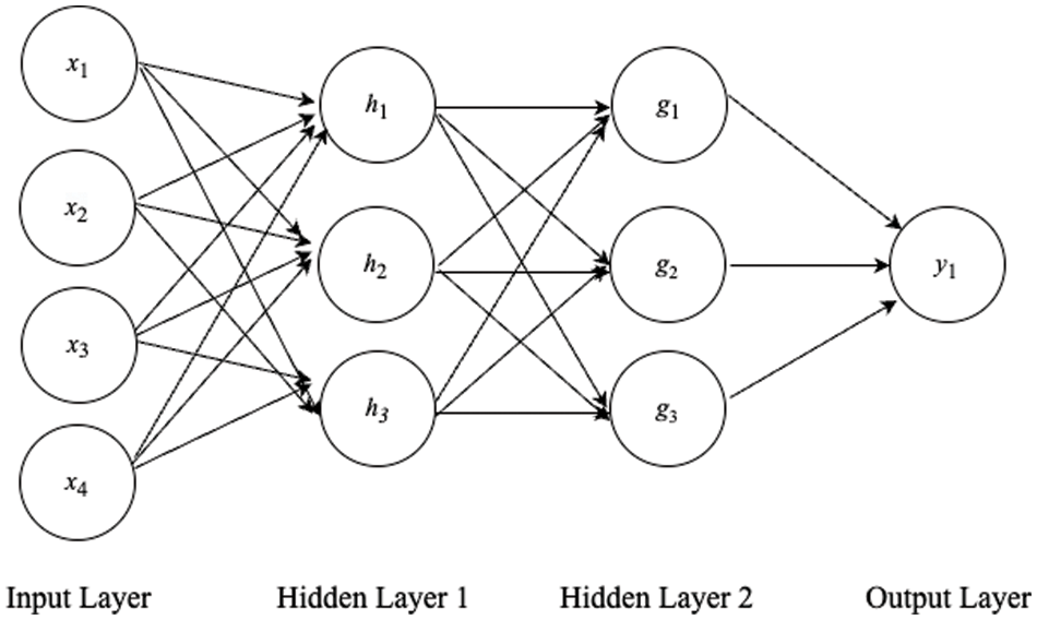
Figure 1: Basic FNN architecture

A CNN is the regularized version of an FNN that builds up with additional convolution layers, pooling layers, and a fully connected layer. CNN is widely applied in image, video, and speech recognition. Abdel-Hamid et al. [15] have found that CNN can reduce the error rate by 6% to 10% when compared with baseline FNN on speech recognition tasks. They indicate that CNN has three key properties: locality, weight sharing, and pooling. The purpose of the convolutional layer and pooling layer from CNN is to extract the significant features, as well as the patterns that can reflect the important components in time series data. In the findings of [9], an NPCNN is the same as the structure of a CNN except for the removal of the pooling layer. Liu et al. have proposed that NPCNN along with rectified linear unit (ReLU) activation function and Adam optimizer performs the best in time series with seasonality and trends since it is an optimal method for both linear and nonlinear datasets and does not require human intervention.

Since the 1990s, an RNN has been one of the important parts of neural network research. An RNN is one class of neural network and is particularly designed for sequence models [16], so it has been widely used to solve time series and ordered data tasks. Nowadays, the application of an RNN can range from sentiment classification to stock price forecasting. Fig. 2 is an RNN architecture that also contains an input layer, 2 hidden layers, and an output layer. Different from an FNN, RNN includes a recurrent network in the hidden layers which can be feedback as input data to the current step. The design of the recurrent network in an RNN enables to capture of the sequential information and storing it in the memory state. In 1990, Werbos introduced the approach of backpropagation Through Time (BPTT), which is the extension of the RNN [17]. BPTT is a gradient-based method to train the RNN as the sequence of the network along with time evolution.

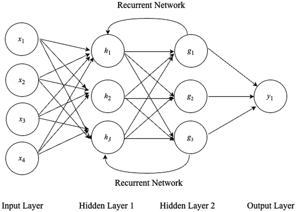
Figure 2: RNN architecture

Employing recurrent networks and BPTT in Vanilla RNN can prove advantageous for short-term time-series forecasting tasks. This is due to its simpler architecture, faster computational complexity, and its tendency to retain recent memories. However, BPTT in RNN usually suffers from exploding and vanishing gradient problems, since the backpropagated error in temporal evolution exponentially increases or decreases based on the size of the weights. The potential problems can cause the oscillating weights and the prohibitive amount of time taken by learning to bridge long time lag [10]. Hochreiter et al. [10] proposed an RNN variant, LSTM, to address the problems, that is enforcing constant error flow through internal states of special units. Moreover, another RNN variant, CW-RNN aims to solve the long-term dependency problem by having different parts of the RNN hidden layer running at different clock speeds, timing their computation with different and discrete clock periods [11]. And yet, updating the neurons in the different clock rates can impact the captures of temporal patterns in the time series forecasting tasks. LSTM is more proper to overcome the long-term dependency problem by its memory cells and gating mechanisms.

Although the adaptability inherent in machine learning models presents some advantages, their effectiveness heavily relies on access to extensive and high-quality datasets, which can be challenging. Some novel time series modeling approaches have been discussed and developed in diverse sectors, including biological systems and chemical processes. For example, the development of a deep hybrid model integrating first integrate first-principles models and deep neural network (DNN) [18,19]; the development of a deep hybrid model integrating universal differential equation and DNN [20,21]; the development of hybrid model integrating time-series transformer framework [22–24]. These hybrid models are designed to enhance comprehensibility predictive accuracy and system-to-system transferability. They also come with principal applications, including the hydraulic fracturing process, intracellular signaling pathways, control in the industrial fermentation process, and crystallization process. We aim to delve into time series forecasting in multiple economic-related domains as well as the versatility of LSTM, inspired by these integrations of machine learning models.

ARIMA was first introduced in the 1970s [25]. In this article, ARIMA is the typical and traditional statistical model used to compare with an RNN. Before applying the ARIMA, it tends to obtain the stationary time series, which means a preprocessing step for non-stationary time series is essential. Liu et al. [9] were not able to show ARIMA modeling results on simulated data until the data was detrended and deseasonalized. In addition, Zhang et al. [12] concluded that the performance of detrended and deseasonalized data in NN models was significantly better than ARIMA. However, a preprocessing step for non-stationary data does not agree with the state-of-art of AutoML.

The assumption over the performance of ARIMA on long-term time series forecasting is not as good as the performance of the RNN, given the fact that the RNN can have internal memory. From the structure of an RNN aspect, the output can be fed back as the input for the next step. In this article, we design and generate experiments with simulated time series data and real data to prove our hypotheses. FNN is considered as the baseline model, to study the effect of recurrent network and BPTT in Vanilla RNN and LSTM. The combination of the ReLU activation function and Adam optimizer is used in all the NNs in our experiments. To obtain a comprehensive analysis of long-term time series in AutoML, we also include the modeling results of the CNN and the NPCNN. The empirical result in this article is one step advance in developing a fully AutoML system with the following three contributions: (1) Full Automation: the proposed system will take pre-processed data input to produce a model as output without human intervention. (2) Adaptability: this system will work for most time series forecasting tasks and automatically searches for the best model configurations. (3) High-quality: this proposed system will offer high-quality models on different types of time series data.

Meanwhile, long-term time series forecasting presents various challenges. The primary limitations encompass: (1) Data quality issues, such as missing values and high intermittency in real-time-series data. (2) External uncertainty, as the accuracy of predicting future values based on historical data proves inadequate. (3) Model degradation, where traditional statistical and certain machine learning models struggle to capture trends and patterns due to the long-term dependency of time series.

The proposed method, utilizing LSTM RNN, showcases improved performance in univariate time series forecasting. In addition, this approach empowers non-professionals to effectively engage in time series forecasting, yielding superior results compared to the traditional ARIMA model crafted by experts in both long-term and short-term scenarios.

The rest of the article is organized as follows. Section 2 reviews the preliminary knowledge of time series, the theoretical foundation of the ARIMA, and multiple neural network systems. Section 3 discusses our research design and explains the setting of multiple NN models and ARIMA. Section 4 gives a comparative analysis and presents empirical results. Section 5 concludes our research, summarizing the findings. In Section 5, we delve into potential future research directions, emphasizing extending our methods to long-term multivariate time series forecasting and time series forecasting involving multiple covariates.

2  Methodology

This section discusses the basis of time series and how the traditional statistical model ARIMA and multiple NNs apply to time series data.

2.1 Seasonality and Trends in Time Series

Time series data can include two important patterns: seasonality and trends. Seasonality occurs in time series when patterns repeat in a fixed period. Trend occurs when long-term time series increases or decreases, and it is usually described with a linear function. Most non-stationary time series data involve seasonal and trended patterns.

The multiplicative decomposition of seasonal and trended time series can be described as Eq. (1).

Xt=Tt×St+et(1)

where at time t, Xt is the value of time series, Tt is the trend component, St is the seasonality component and et is the noise. Before analyzing seasonal and trended time series, the decomposition of the time series is essential. Seasonality can be presented by the plot of the partial autocorrelation function for each seasonal lag. The trend can be explained by the correlation between Xt and Xt−k, where k is the length of the cycle.

With neural networks, no specific assumptions need to be made about the model, and the underlying relationship is determined solely through data mining [12]. NN can automatically recognize seasonal and trend patterns.

2.2 Autoregressive Integrated Moving Average (ARIMA) and Seasonal ARIMA

ARIMA and seasonal ARIMA are traditional statistical approaches to forecasting time series data. If time series is non-stationary, decomposition of time series has been applied to remove the effects of seasonality and trend.

ARIMA (p,d,q) is a classical statistical method that is generalized by the integration of Autoregressive (AR) and Moving Average (MA) and makes the non-stationary data stationary by taking the difference between current data values and previous data values. p is the order of AR, d is the degree of differencing and q is the order of MA. For trended time series, ARIMA (p,1,q) takes the degree of 1 difference of the time series values as Eq. (2).

Δyt=yt−yt−1(2)

where yt is the future value and yt−1 is the previous value.

The work by Box et al. [25] on the seasonal ARIMA model has had a major impact on the practical applications of seasonal time series modeling. ARIMA model needs that data to be seasonally differenced to satisfy the stationarity condition. In the ARIMA (p,d,q)×(P,D,Q)s model, p,d,q represent nonseasonal factors and P,D,Q represent seasonal factors. Thus, the ARIMA (p,d,q)×(P,D,Q)s model follows Eq. (3).

ΦP(Bs)ϕ(B)∇sD∇dxt=δ+ΘQ(Bs)θ(B)wt(3)

where s is the length of the cycle, the polynomials ϕ(B),θ(B) of orders p,q respectively represent the AR part and MA part, ΦP(Bs),ΘQ(Bs) of orders P,Q respectively represent the seasonal AR part and seasonal MA part, ∇d=(1−B)d is the nonseasonal component and ∇sD=(1−Bs)D is a seasonal component.

To address seasonality and trends in time series, human intervention is required if applying ARIMA to model time series. We need to manually select the parameters p,d,q,P,D,Q of ARIMA when we solve every time-series task. However, neural network models can give more efficient solutions, since the selection of parameters is no longer needed and particular assumptions are unnecessary for modeling. Thus, deep learning can determine and investigate the underlying relationship of time series data. This data-driven approach is one of the most important advantages of neural networks in solving many complex real-world forecasting problems [12].

2.3 Fully Connected Network (FNN)

A FNN is a basic neural network model that contains only fully connected layers. Fully connected layers can employ the different activation functions, to have linear or nonlinear transformation to an input vector along with weight matrix and bias. Fully connected layers are usually placed at the end of the sequence of layers in NNs, so they generate the outputs. For the time series forecasting tasks, the input nodes are the previous lagged observations while the output provides the forecast for the future value [12]. Simply, the model can be expressed mathematically, for m is the number of input nodes, n is the number of hidden nodes,

yt=α0+∑j=1n(∑i=1mβijyt−i+β0j)+ϵi(4)

where yt,yt−i are future values and previous lagged observations respectively, f can be some activation functions, α0,β0j are the bias terms, αj is the weight vector from hidden layers to the output layer, and βij are weights from the input layer to hidden layers.

The fully connected layers can be applied in hidden layers to transform the inputs to higher dimensional data to prepare for the other NN models.

2.4 Convolutional Neural Network (CNN)

CNN is a regularized version of FNN that contains convolution operation and pooling operation. The purpose of the convolution layer is to extract the features from the input data. A filter or convolutional kernel is a smaller matrix in spatial dimensionality. The convolution layer convolves each filter across the dimensions of input to produce a two-dimensional activation map [26]. As the filters slide through the entire input data, element-wise multiplication is operated at each corresponding region. Thus, it generates a feature map that can highlight and capture learned features. A CNN uses convolution in at least one of its layers. The flexibility of the CNN can be well modeled for image classification, video recognition, time series, etc. As we introduce the specific attributes of FNN previously, the networks are fully connected and tend to overfit the data. The pooling layer is organized into feature maps, and the number of feature maps in the pooling layer and in the convolutional layer are the same, except the size of the map is smaller. The purpose of the pooling layer is to reduce the resolution of feature maps [15]. A CNN takes another approach to regularize NN that finds the hierarchical pattern in the data, extracts the internal components, and uses simpler and smaller patterns to compose another pattern.

We intend to use a CNN to predict the future value X_t in the time series. Given any time series, the equation follows Eq. (5).

Xt=f(Xt−1,Xt−2,⋯,Xt−k)+εt(5)

where Xt−1,Xt−2,⋯,Xt−k are the previous lagged observations, f are some functions and εt is the error. The previous lagged observations are fed into hidden layers to extract and pattern. CNN’s framework performs well in terms of discovering and extracting the internal structure of data [27].

2.5 Nonpooling Convolutional Neural Network (NPCNN)

The structure of an NPCNN is the same as the structure of a CNN, except for removing the pooling layer, which makes NPCNN contain convolutional layers and fully connected layers. What is the contribution of the pooling layer in CNN? The very success of CNNs on visual object recognition tasks was thought to depend on the interleaved pooling layers that purportedly rendered these models insensitive to small translations and deformations [27]. The pooling layer allows representations to vary very little when elements in the previous layer vary in position and appearance [28]. In CNN, the pooling layers can cause the loss of information, but it can be neglected if we aim for image classification.

Being different from image classification, we do not want to lose some important information when it comes to time series forecasting. In [9], Liu et al. have studied and reported the effects of convolutional layers and pooling layers in CNN. Their empirical results provide an important suggestion when modeling seasonal and trended time series with CNN to avoid pooling layers in the network.

2.6 Backpropagation Through Time (BPTT) and Recurrent Neural Networks (RNN)

An RNN is a type of ANN that allows previous outputs to be fed as inputs to the current step within the hidden layers. The recurrent connections in the RNN allow saving the “memory” from the past to predict current and future data values, so the effect of recurrent networks brings particular advantages to the RNN. Therefore, RNNs are widely applied in sequential and time series data.

Distinguished from the other NNs, the weights of parameters in the RNN are the same within the network, because the gradients from outputs at the current time step are dependent on outputs from the previous time step. Thus, it can reduce the complexity of parameters. The weight of parameters can be determined and adjusted by the BPTT algorithm. BPTT is an extension to basic backpropagation, and it can be applied to dynamic systems. This allows one to calculate the derivatives needed when optimizing an iterative analysis procedure, a neural network with memory, or a control system that maximizes performance over time [17]. For instance, in the dynamic system, if we need to recognize moving objects in the NN, the action at time t is required and determined by the memory at time t−1.

The loss function ℒ in the RNN at all times depends on all the loss at each time step, and the math expression follows Eq. (6).

ℒ(y^,y)=∑t=1Tℒ(y^⟨t⟩,y⟨t⟩)(6)

Furthermore, the BPTT algorithm computes the gradient at each time step t using the loss function, such as Eq. (7).

∂∂Wℒ(𝒯)=∑t=1T∂∂Wℒ(𝒯)|(t)(7)

where W is the weight matrix.

Fig. 3, [28] presents the unfolding RNN in time and the complete computation process in the RNN structure.

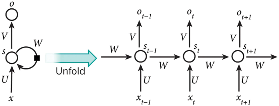
Figure 3: Unfolding RNN (LeCun et al. [28])

Note that xt is the input at time step t, st is the hidden state at the time step t and the black box is the delay of one time step. As a result, it has become the internal memory in the RNN. st can be calculated as Eq. (8).

st=f(Uxt+Wst−1)(8)

Also, ot is the output at time step t and the same parameters (U,V,W) are shared across the time. To forecast the future data values in the time series data, applying the activation function can generate the output at each layer of RNN.

2.7 Long Short-Term Memory (LSTM)

Hochreiter and Schmidhuber [10,29] discovered the vanishing and exploding gradient problems in the Vanilla RNN. According to the gradient-based algorithms, such as Real-Time Recurrent Learning and BPTT, the gradients of the loss function can become smaller and converge to zero; become larger, and diverge, as the current error signals backpropagate in time. Hence, LSTM is introduced with memory cells and gate units to solve the long-term dependency problems and improve long-term time series forecasting tasks.

A memory cell block consists of an input gate, a forget gate, and an output gate. S memory cells sharing the same input gate and output gate form a structure called a “memory cell block of size S”. The input gate is to store and protects the memory information from perturbation by unnecessary input. The forget gate is to look for and discard information from the block. The output gate can determine what memory to remove from the block. The gate units aim to control the error flow from input connections to output connections [10]. Fig. 4 illustrates the operational principles and roles of memory cells within an LSTM architecture. The system comprises 8 input units, and 2 memory cell blocks of size 2, along with 4 output units. Within the layers, each gate unit and memory cell can see all non-output units. Given a sequential data input, the networks initialize the input and form the memory cells and gate units. Within the memory cells, it takes inputs at the current time step and applies the activation function to connect the previous hidden state at the input gate; discards the irrelevant memory at the forget gate and updates memory; it leads updated memory to the output gate. Then, it can output the current values based on passing the previous states.

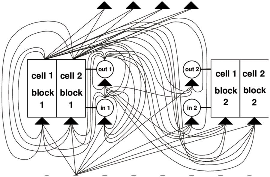
Figure 4: Memory cell in LSTM architecture (Hochreiter and Schmidhuber [10])

Therefore, during the BPTT, the gradients can propagate unrestrictedly through the three gates within the memory cell. Thus, it involves multiple learnable parameters: input weights, recurrent weights, and bias terms. Across the multiple time steps, it allows us to learn and update each parameter in LSTM while training to minimize the error. Hence, the LSTM system is better at retaining useful long-term memory and not losing short-term memory.

2.8 Rectified Linear Unit (ReLU) Activation Function & Adam Optimizer

Activation functions are well developed to apply in NNs, and some activation functions are most commonly used, such as linear function, ReLU, and Sigmoid function.

The purpose of the non-linear activation function in NNs is to generate non-linear output in the model. ReLU is one of the activation functions in deep learning, which indicates the non-linear function. It aims to resolve the vanishing gradient problem in the RNN. The definition of ReLU is expressed as the positive part of the argument and its mathematical expression of ReLU is

f(x)=x+=max(0,x)(9)

where x is input to a neuron in NN.

Adam optimizer is an optimization algorithm that is the derivation of stochastic gradient descent. It is used to update weights iterative in the NNs. In a large number of recent deep learning studies, Adam optimizer is shown empirically to outperform the other gradient-based and stochastic gradient-based optimization methods.

The empirical findings have shown and suggested that the combination of ReLU activation function and Adam optimizer is the best and most efficient when modeling in the baseline FNN [9]. Therefore, in Section 3, we will adopt this combination in all of the NN models.

3  Research Design

This section presents the experiment setting of ARIMA and NN models, demonstrates the potential challenges of long-term time series forecast using simulated data and real data, and provides the modeling strategy to overcome the challenges. Both simulated data and real data are trended and seasonal, so how the models address these two components in the time series is important to our study.

In the experiment, ARIMA serves as the traditional statistical model, which is widely applied to time series forecasts. At the same time, FNN serves as the baseline model for the NNs, since its structure is simple and direct. The characteristics and capabilities of CNN, NPCNN, and RNN can be specified when constructing the neural network system. The purpose of this article is to provide the empirical results, so two main questions are investigated as follows:

1.    How is the data preprocessing conducted in the ARIMA and NNs? Will data preprocessing significantly improve the forecasting performance?

2.    Is an RNN able to overcome the trends and seasonality components of time series, and outperform the traditional statistical method ARIMA and other NNs in long-term time series forecasting?

3.1 The Simulated Data

The idea of simulated time series data was originally adopted from [12], but the simulated data needs to be generated and adjusted following our research goals.

The data uses month as a unit, so it can be closely and commonly applied to economic and business real data. Additionally, monthly time series are more challenging for forecasts, because they have more seasons to deal with the other types of seasonal data such as quarterly time series [12]. Similar to Eq. (1), the mathematical expression of the multiplicative model follows Eq. (10).

yt=Tt×SIt+et(10)

where at time t, Tt=100+0.6t represents the linear trend components, SIt represents seasonal components referred to in Table 1, and et represents the error term using the Gaussian noise N(0,σ2). Among the options of σ=1,5,15, σ=15 is selected, because the range of noise distribution can be larger and the simulated time series is closer to real data.

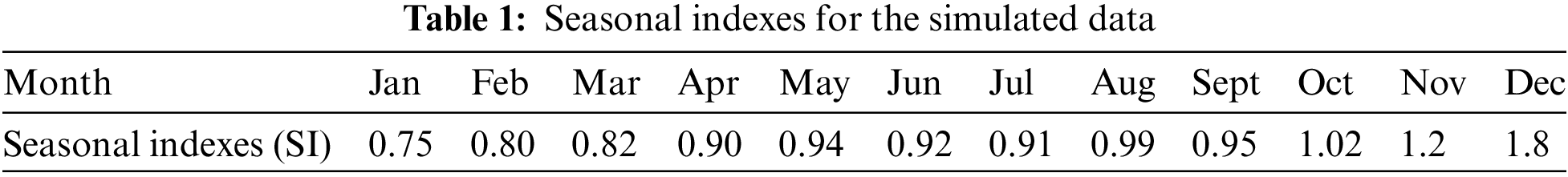
The long-term time series forecasting task is difficult and unexpected. Instead of simulated data having a stable linear growth, we decided to modify the data by increasing 40% values from t=156 to t=180. The purpose of modification is to make the simulated data more complex, so it can mimic some real data. Fig. 5 is shown as the plot of the simulated time series after the adjustment.

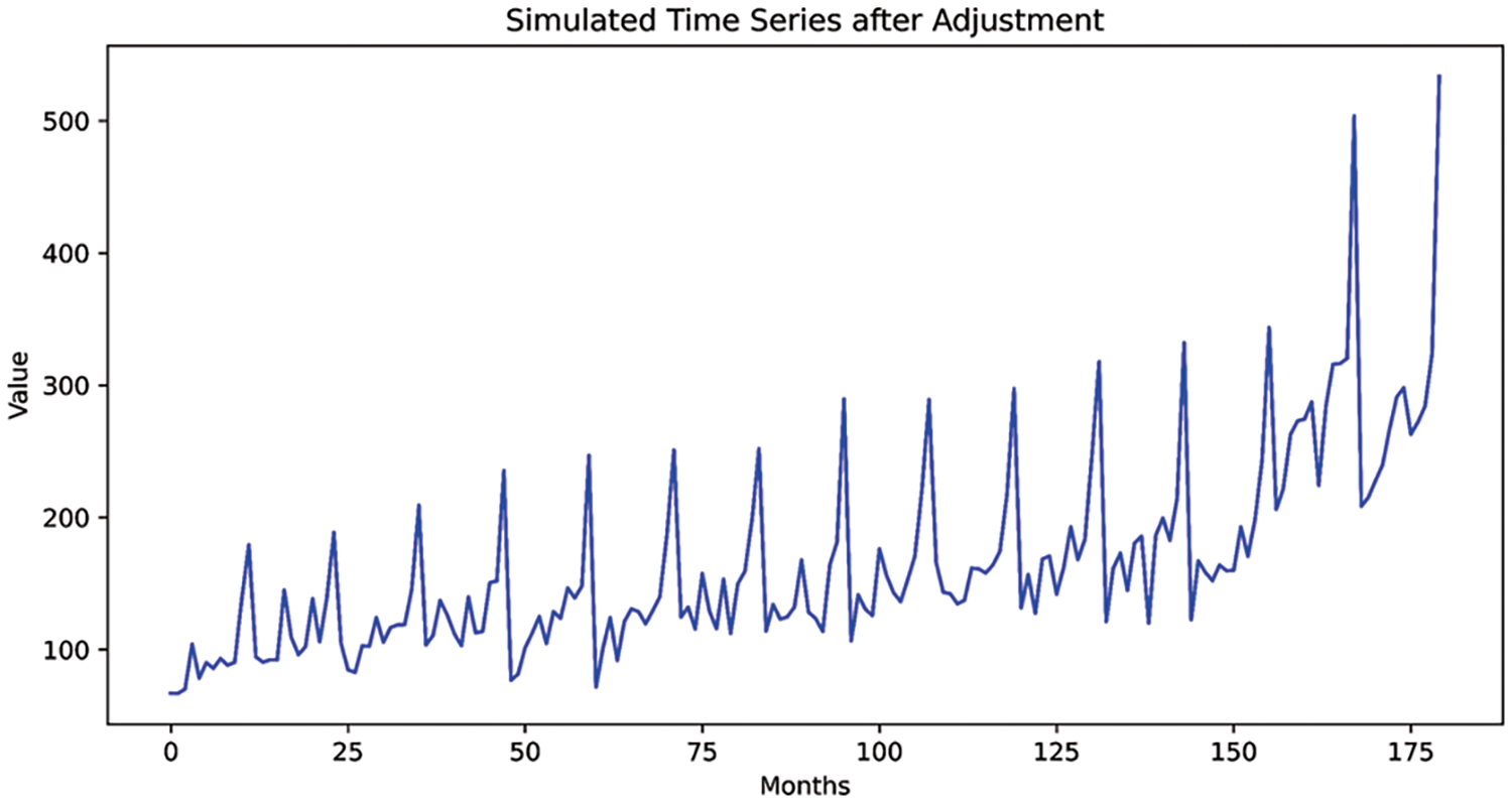
Figure 5: The simulated time series after adjustments

The total number of simulated data points is 180. For data partition, the training set includes the first 156 data points, and the test set includes the remaining 24 data points. As a result, data splits in such form of a 156-months training set and a 24-months test set (unknown forecast lengths).

3.2 The Real Data

The real data is the monthly wine sales collected by the database of analytical results of the Australian Wine Research Institute’s Commercial Services Group [30]. Both real data range from January 1980 to December 1994, and the dataset includes white wine sales and red wine sales in such time order. Fig. 6 shows the plots for white wine sales and red wine sales, respectively.

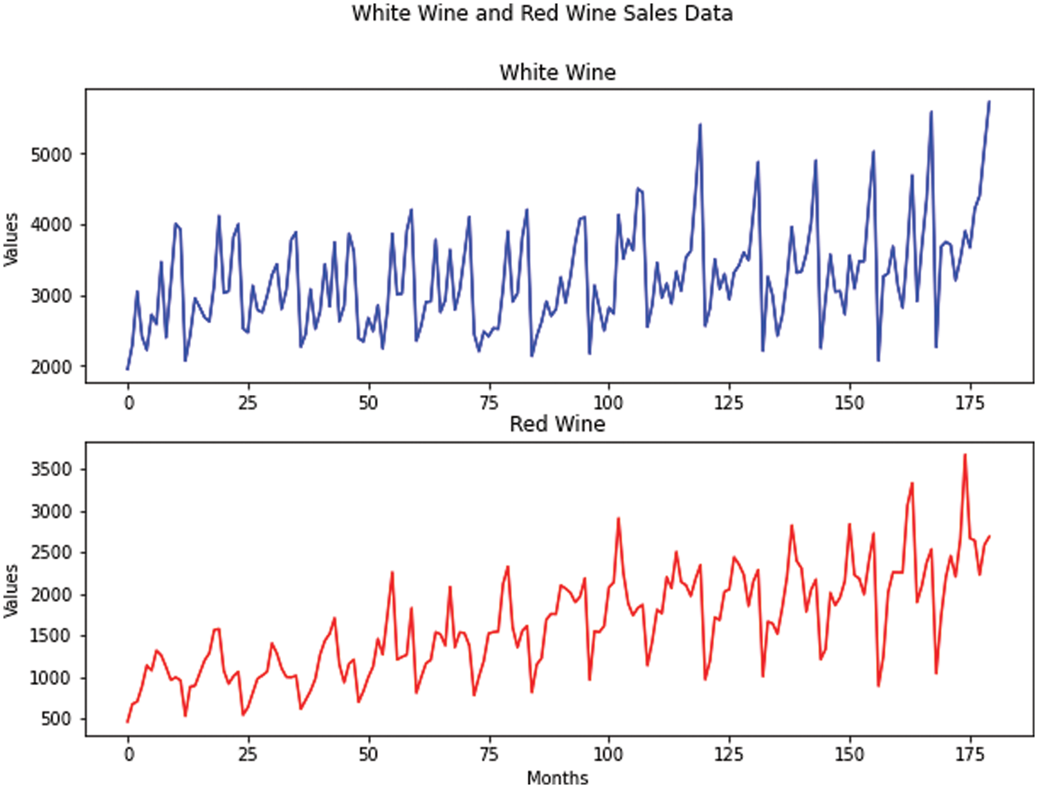
Figure 6: The real data

In this study, white wine sales and red wine sales are both treated as independent univariate time-series data and thus, the correlation between white wine sales and red wine sales is not considered.

The number of simulated data points is the same as the number of each real dataset. Similarly, the data partition for each real dataset follows: the training set includes the first 156 data points and the test set includes the remaining 24 data points.

3.3 Modeling Strategy

The modeling strategy discussion is separated into two parts: how to develop the traditional statistical model ARIMA and how to develop the deep learning model NNs.

At first, it is essential to determine if the time series is stationary before modeling ARIMA. To determine if the time series data is stationary, the Augmented Dickey-Fuller (ADF) test is commonly applied. The ADF is the extension of the Dickey-Fuller test, so the model of ADF is given as Eq. (11).

Δyt=c+βt+γyt−1+δ1Δyt−1+⋯+δp−1Δyt−p+1+εt(11)

where c is a constant, β is the coefficient for trend and p is the lag order of the AR process.

The ADF is used to test the null hypothesis assuming the presence of unit root in the time series. With significance level α=0.05, if the p-value calculated from Eq. (10) is greater than α=0.05, then we can conclude this time series is stationary; otherwise, it is non-stationary.

A time series needs to lack trend and seasonality to be stationary, where the trend and seasonality may affect a time series at different instants and result in inaccurate predictions [31]. Therefore, the preprocessing step of deseasonalization and detrend (DSDT) of non-stationary time series is necessary before proceeding to ARIMA.

The results of the ADF test show that simulated data and both real data are non-stationary time series. Given a range of parameters in ARIMA (p,d,q)×(P,D,Q)s, it requires to use grid search algorithm to target the best combination of parameters’ values among all the possible combinations. Grid search can be used with ARIMA and other models where it proved efficient. It tries a set of possible hyper-parameters applied to the task at hand [2]. However, grid search algorithms can be computationally expensive and require enough manual effort. Each time series modeled by ARIMA has to experience the grid search because the ARIMA results in different parameter combinations for different time series data.

For the simulated data and both real data, the ARIMA model is trained using the 156-month training set and aims to predict a 24-months test set. Details of empirical findings will be provided in the next section.

Secondly, let us discuss the experimental setting for NNs. Please note all of the neural network models are applied by the open-source software Keras and TensorFlow.

In our research, a FNN is considered a baseline model among all the NNs. The construction of CNN, NPCNN, Vanilla RNN, and LSTM will be modified based on the construction of FNN. Although we notice that simulated data and wine sales data are non-stationary, the state-of-the-art AutoML and NN systems do not require time series deseasonalization and detrend, so this data preprocessing step can be omitted. Moreover, data normalization can be applied based on the nature of the task. To train neural networks with univariate time series data on the Keras interface, the scaled training set needs to be proceeded to TimeseriesGenerator. Thus, a univariate time series can generate batches of input-output pairs. The input_shape in the modeling includes length of 12 with 1 feature. To keep the consistency of the experiment, the process of obtaining the input and output pairs should be consistent for the test set. Furthermore, the input data needs to be reshaped to proceed to the input layer according to the characteristics of a certain type of layer. The FNN in the experiment includes 4 layers: an input layer based on the shape of generated_batches, 2 hidden layers (Dense(64) and Dense(16)) both using ReLU activation functions, and an output layer using Linear activation function. On the Keras interface, an FNN is constructed by multiple dense layers and the number of neurons or units can be selected based on the complexity of the problem. Dense(64), one of the hidden layers, represents that the output space dimension is (None, 64). Then, (None, 64) becomes input, proceeds to the next hidden layer, and Dense(16) generates the output as (None, 16). The neurons in each layer contain the weight and bias, so backpropagation is used to learn them. ReLU is not linear, thus it has the flexibility to make the arbitrary shape and approximate the domains. In the output layer of FNN, Dense(1) with Linear activation function is used, since it aims to solve the regression problem. The model is compiled by defining the Adam optimizer and mean absolute error (MAE) loss. It indicates that the loss will be minimized by the optimizer during the training process.

A CNN is constructed based on the construction of FNN. Other than the layers in the FNN, one convolutional layer with 8 convolutional kernels (Conv1D) and ReLU activation function, and one pooling layer with ReLU activation function (MaxPooling1D) are added in the hidden layers. When training CNN, time series data is considered as one dimensional or flattened image, thus we use Conv1D and the number of convolutional kernels indicates the length of the one-dimensional convolution window. Reference [9] tested the uses of two types of pooling layers with the metrics mean square error (MSE): AveragePooling1D and MaxPooling1D, and the results of MaxPooling1D show the lowest errors. In addition, to proceed to the Conv1D layer, the shape of inputs required to be three-dimensional with batch size, the number of timesteps, and the number of features. The use of the pooling operation in CNN is to downsample and reduce the inputs, so it helps avoid overfitting. Since the dimension of inputs is a three-dimensional tensor, CNN should flatten (Flatten) the inputs, so it can well proceed to the output layers with the Linear activation function.

The construction of NPCNN is the same as CNN, except for removing the pooling layer (MaxPooling1D). To consider the effect of seasonality and trends, the removal of the pooling layer can improve the long-term forecasting results. The details are discussed in Section 4.

Given the FNN as the baseline, a fully connected RNN layer with 128 neurons and ReLU activation function (SimpleRNN) is added and the remaining layers remain the same as in FNN. The shape of inputs should be based on generated_batches by the TimeseriesGenerator, but SimpleRNN outputs in the two-dimensional form, so a flattened layer is not necessary for RNN. The reason for that is the fully connected RNN layer processes input sequences one-time step at a time and produces an output vector for each time step. Furthermore, the output vector of each time step becomes a function of the input vector of that time step and the internal state which RNN particularly owns. However, a Vanilla RNN can easily suffer from learning dependencies. To improve the performance, we can highly recommend an LSTM. It is an RNN variant, so it can be superior compared to the other methods because its internal state can be updated based on previous “memory” and current inputs, and also retain the long-term dependency. From the efficiency perspective, LSTM is more computationally intensive than Vanilla RNN, because of the memory cells and gate mechanisms. The experimental diagram is given by Fig. 7A, in order to clearly demonstrate our computational approach. When constructing LSTM networks as Fig. 7B, the LSTM layer is selected in addition to the FNN baseline model.

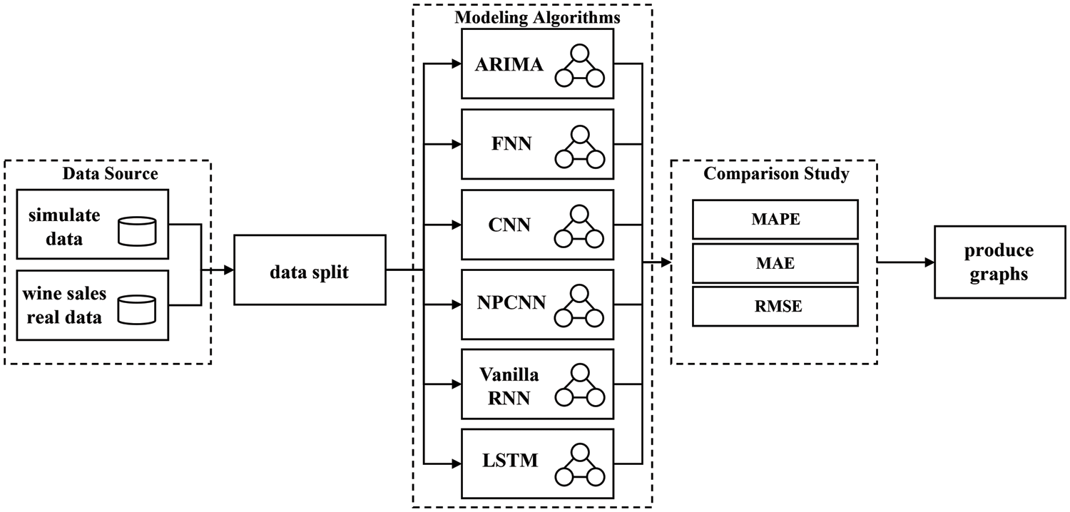
Figure 7A: Experimental diagram

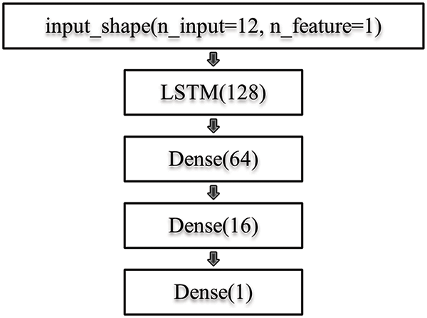
Figure 7B: LSTM structure

4  Empirical Findings

The previous section introduces the simulated data and both real data and discusses the experimental setting of ARIMA and NNs, so this section aims to show and interpret the empirical results from the experiments. The empirical results include the performances and visualizations of long-term forecasts of the test set. In the experiment, the evaluations of models are not only on the whole test set, but evaluations of the first 6, 12, 18, and 24-month data of the test set are also shown.

Three accuracy metrics are used for model evaluation: (1) Mean Absolute Percentage Error (MAPE), (2) MAE, and (3) Root Mean Square Error (RMSE). The formulas of metrics follow Eqs. (12)–(14).

MAPE=100%⋅1n∑t=1n|Yt−Yt^Yt|(12)

MAE=1n∑t=1n|Y^t−Yt|(13)

RMSE=1n∑t=1n(Yt−Y^t)2(14)

where t is time, Y^t is the predicted value at t and Yt is the observed value at t.

MAE and MAPE are more important measurements in the time series modeling evaluation. To observe if there is any inconsistency in modeling performance, MSE and RMSE are also applied and referred to. MSE and RMSE are commonly used to evaluate the models, so they do not need more discussion. MAPE is capable of measuring the mean percentage difference between the predicted values and observed values. For example, if MAPE is 4%, then the average prediction is 4% off the observed value, so the purpose of MAPE is to bring the relative measures in the model. MAE can directly measure the mean absolute difference between the predicted values and observed values, so its clear interpretability helps obtain the magnitude of errors.

4.1 The Results of Modeling Simulated Data

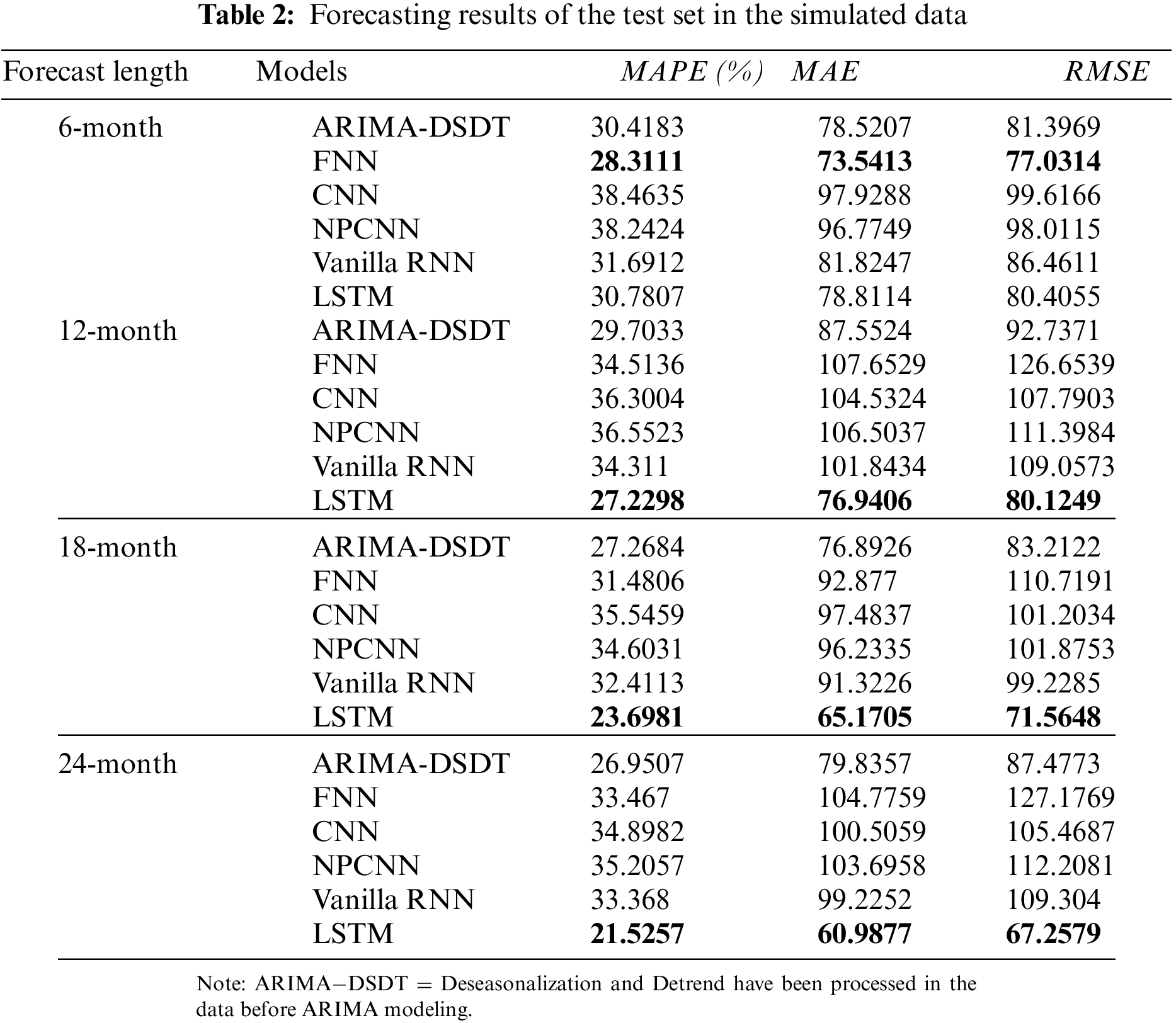
Table 2 shows the forecasting results of 6, 12, 18, and 24-month in the test set. For the 6-month forecasts, the forecasting errors from CNN and NPCNN are not far different, but both of them have the highest errors. The forecasting errors from ARIMA, Vanilla RNN, and LSTM are very close to each other, but the errors of FNN show to be the lowest. However, for 12, 18, and 24-month forecasting, the forecasting errors of LSTM outperform all the other NNs and ARIMA by resulting lowest errors. Particularly, the errors of LSTM are approximately 40% or less than the errors of FNN, CNN, NPCNN, and Vanilla RNN, and on the other hand, the performance of ARIMA is better than these NNs. The overall performance of NPCNN is slightly better than CNN, due to the removal of the pooling layer. As more months we predicted, the errors of all models increased, so it indicates more difficulty encountered when predicting long-term time series.

According to the Fig. 8, the ARIMA (3,1,0)×(0,1,1)s and LSTM predictions do show capturing and well predicting the abrupt increase in the simulated data, but prediction by LSTM eventually and approximately reaches to actual value as time passes. LSTM shows itself to be a more reliable and flexible tool when forecasting long-term time series.

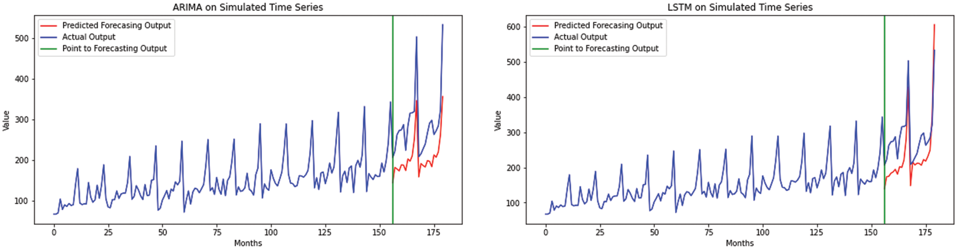
Figure 8: The simulated data forecasting compared by ARIMA (3,1,0)×(0,1,1)s and LSTM

4.2 The Results of Modeling Real Data

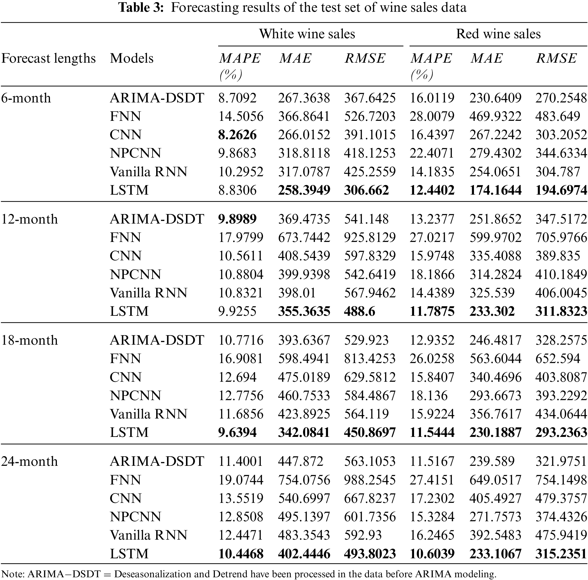
The evaluation design of real data is similar to the simulated data. Firstly, for the white wine sales data, Table 3 shows that forecasting errors of ARIMA and CNN are the closest to the errors of LSTM, ARIMA and CNN slightly better predict the short-term forecasted values. However, the forecasting errors of FNN are shown to be one time higher than them. The white wine sales data does not reveal enough linear trend but obvious seasonality. The long-term forecasting results of LSTM outperform in terms of all three metrics. Nevertheless, the long-term forecasting performance of CNN and NPCNN is not satisfying, compared to the others. The 24-month prediction by LSTM computes that is approximately 10.45% off the observed values, and thus this long-term forecast is promising.

Moreover, Fig. 9 shows that RNN forecasts are well able to capture small fluctuations of the sequence which ARIMA is not.

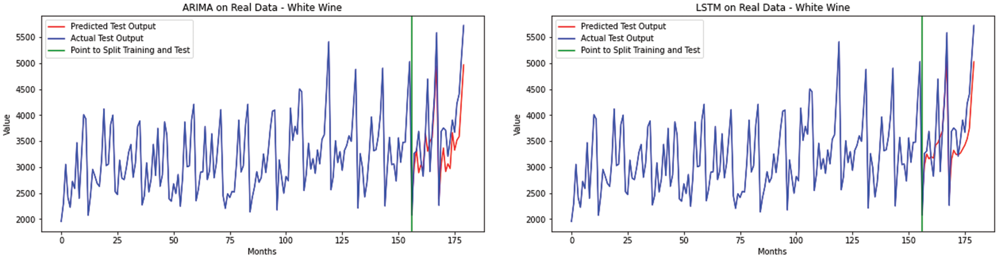
Figure 9: The white wine sales data forecasting compared by ARIMA (0,1,1)×(0,1,1)s and LSTM

The red wine sales data shows a more obvious trend and seasonality, compared to white wine sales data. Table 3 also shows that the forecasting errors of ARIMA are closer to the forecasting errors of Vanilla RNN and LSTM in the red wine data. None of FNN, CNN, and NPCNN do not perform satisfyingly in short and long-term forecasting, compared with ARIMA and LSTM.

Table 3 also indicates that the overall performance of NPCNN is not as satisfying as CNN. The LSTM also outperforms in all lengths of forecasting. After time series deseasonalizing and detrending, ARIMA can be competitive among the model selections. In Fig. 9, the visualization of ARIMA and RNN forecasts can attest. To forecast red wine sales data, the errors of FNN point out that FNN might encounter more challenges due to larger effect seasonality and trend components.

4.3 Critical Analysis and Discussion

One significant advantage of this approach is its user-friendly design, allowing individuals without expertise in ARIMA to engage in univariate time series forecasting through the application of an LSTM network. The practical demonstration of this methodology using real-world data illustrates its effectiveness in achieving superior forecasting outcomes for both short-term and long-term scenarios.

However, it is important to note that this approach has its limitations. Users are still required to possess knowledge of LSTM networks and the ability to fine-tune their parameters to ensure satisfactory results.

In the realm of time series forecasting, widely employed in various commercial applications, a significant barrier exists—many data scientists lack expertise in time series analysis, such as ARIMA. Furthermore, the accuracy of long-term forecasting using ARIMA is often insufficient, limiting its widespread application. The impactful contribution of this approach is democratizing both long-term and short-term time series forecasting, providing data scientists with superior performance capabilities.

5  Conclusion

Nowadays, time series analysis and forecasting have been studied by more techniques such as traditional statistical methods, machine learning, and deep learning. The automated search can adjust the architecture and hyperparameter choices for different datasets, which makes the AutoML solution generic and automates the modeling efforts [1]. The automatic machine learning framework suggests that non-professionals can solve machine learning-related problems efficiently, and require less human intervention and effort.

Meanwhile, the purpose of this study is to provide a solution in terms of AutoML novelty when solving long-term time series tasks. This article has provided a detail-oriented analysis between classical statistical model ARIMA and multiple NNs, and empirically shown the ability and significance of neural network models on the seasonal and trended time series. The finding of [32] reveals how competitive are neural networks in time-series forecasting compared with traditional univariate methods.

The decomposition of non-stationary time series is required for the ARIMA model, and the data preprocessing cannot be neglected. In the experiment of ARIMA, they result in different parameters for each simulated data and real data, because the grid search of parameters is necessary to obtain the best combination of parameters. Moreover, traditional statistical models usually require users to have statistical and mathematical knowledge, to better practice in real life. On the other hand, the advantages of NNs are more compelling. The original time series data can proceed to NNs directly without making it stationary. This article has introduced the fundamental basis and experiments of FNN, CNN, NPCNN, Vanilla RNN, and LSTM, and the characteristics of RNN and LSTM, internal state, and memory cells, bring a major impact in the forecasting. Since the utilization of RNN to perform long-term forecasting, we do not need to hand-craft model parameters such as lag variables used in the ARIMA model. This enables this approach to be used to develop the AutoML system. Even though the long-term forecast by LSTM outperforms, we also have recognized some drawbacks of using LSTM to forecast long-term time series. The training process is complex due to optimizing the hyperparameter in each layer, overfitting can happen during training and the deep learning model often lacks interpretability.

The AutoML approach employing LSTM RNN can yield highly accurate results for both short-term and long-term time series forecasting. And yet, users of this AutoML approach are required to possess certain fundamental knowledge of time series, LSTM RNN and programming skills. This AutoML approach empowers non-professionals to achieve highly efficient univariate time series forecasting, applicable across diverse domains, including sales, marketing and other commercial applications. Consequently, it facilitates the availability of highly accurate time series forecasting for a wide range of commercial applications.

In this article, the empirical evidence has shown the effectiveness of using RNN to perform long-term forecasting on univariate time series. Two nature extensions of this experiment are using RNN to perform long-term multivariate time series forecasting and to perform long-term univariate time series forecasting with multiple covariates. Both cases are more useful than univariate time series forecasting. In addition, this can make AutoML on time series data more practical. Using RNN in both cases is the natural next step for the extension of this study.

Acknowledgement: We extend our gratitude to the invaluable suggestions provided by the reviewers and editors. Thanks to their insightful feedback, this article has undergone substantial improvements. Also, thanks for the support from Prof. Xueli Wang, she provided valuable advise to improve this article.

Funding Statement: The authors received no specific funding for this study.

Author Contributions: The authors confirm contribution to the paper as follows: study conception and design: Morgan C. Wang, Shuai Liu; data collection: Ying Su; analysis and interpretation of results: Ying Su, Morgan C. Wang; draft manuscript preparation: Ying Su. All authors reviewed the results and approved the final version of the manuscript.

Availability of Data and Materials: The dataset used in this paper are available in reference [30].

Conflicts of Interest: The authors declare that they have no conflicts of interest to report regarding the present study.

References

1. C. Liang and Y. F. Lu, “Using automl for time series forecasting,” 2020. [Online]. Available: https://www.googblogs.com/using-automl-for-time-series-forecasting/ (accessed on 04/01/2024). [Google Scholar]

2. A. Alsharef, K. Aggarwal, Sonia, M. Kumar, and A. Mishra, “Review of ML and AutoML solutions to forecast time-series data,” Arch. Comput. Method Eng., vol. 29, no. 7, pp. 5297–5311, 2022. doi: 10.1007/s11831-022-09765-0. [Google Scholar] [PubMed] [CrossRef]

3. T. Tornede, A. Tornede, M. Wever, and E. Hüllermeier, “Coevolution of remaining useful lifetime estimation pipelines for automated predictive maintenance,” in Proc. 2021 Genetic Evol. Comput. Conf., 2021, pp. 368–376. [Google Scholar]

4. T. Elsken, J. H. Metzen, and F. Hutter, “Neural architecture search: A survey,” J. Mach. Learn. Res., vol. 20, pp. 55, 2019. [Google Scholar]

5. I. Y. Javeri, M. Toutiaee, I. B. Arpinar, J. A. Miller, and T. W. Miller, “Improving neural networks for time-series forecasting using data augmentation and automl,” in 2021 IEEE Seventh Int. Conf. on Big Data Comput. Serv. Appl. (BigDataService), IEEE, 2021, pp. 1–8. [Google Scholar]

6. T. Halvari, J. K. Nurminen, and T. Mikkonen, “Robustness of automl for time series forecasting in sensor networks,” in 2021 IFIP Netw. Conf. (IFIP Networking), Espoo and Helsinki, Finland, 2021. [Google Scholar]

7. J. J. Kurian, M. Dix, I. Amihai, G. Ceusters, and A. Prabhune, “BOAT: A bayesian optimization automl time-series framework for industrial applications,” in 2021 IEEE Seventh Int. Conf. on Big Data Comput. Serv. Appl. (BigDataService), IEEE, 2021, pp. 17–24. [Google Scholar]

8. S. Meisenbacher et al., “Review of automated time series forecasting pipelines,” Wiley Interdiscip. Rev. Data Min. Knowl. Discov., vol. 12, no. 6, pp. e1475, 2022. doi: 10.1002/widm.1475. [Google Scholar] [CrossRef]

9. S. Liu, H. Ji, and M. C. Wang, “Nonpooling convolutional neural network forecasting for seasonal time series with trends,” IEEE Trans. Neural Netw. Learn. Syst., vol. 31, no. 8, pp. 2879–2888, 2020. doi: 10.1109/TNNLS.2019.2934110. [Google Scholar] [PubMed] [CrossRef]

10. S. Hochreiter and J. Schmidhuber, “Long short-term memory,” Neural Comput., vol. 9, no. 8, pp. 1735–1780, 1997. doi: 10.1162/neco.1997.9.8.1735. [Google Scholar] [PubMed] [CrossRef]

11. J. Koutnik, K. Greff, F. Gomez, and J. Schmidhuber, “A clockwork RNN,” in Int. Conf. Mach. Learn., Beijing, China, vol. 32, 2014, pp. 1863–1871. [Google Scholar]

12. G. P. Zhang and M. Qi, “Neural network forecasting for seasonal and trend time series,” Eur. J. Oper. Res., vol. 160, no. 2, pp. 501–514, 2005. doi: 10.1016/j.ejor.2003.08.037. [Google Scholar] [CrossRef]

13. G. E. Hinton, “How neural networks learn from experience,” Sci. Am., vol. 267, no. 3, pp. 144–151, 1992. doi: 10.1038/scientificamerican0992-144. [Google Scholar] [PubMed] [CrossRef]

14. C. Paoli, C. Voyant, M. Muselli, and M. L. Nivet, “Forecasting of preprocessed daily solar radiation time series using neural networks,” Sol. Energ., vol. 84, no. 12, pp. 2146–2160, 2010. doi: 10.1016/j.solener.2010.08.011. [Google Scholar] [CrossRef]

15. O. Abdel-Hamid, A. R. Mohamed, H. Jiang, L. Deng, G. Penn and D. Yu, “Convolutional neural networks for speech recognition,” IEEE/ACM Trans. Audio, Speech, Language Process., vol. 22, no. 10, pp. 1533–1545, 2014. doi: 10.1109/TASLP.2014.2339736. [Google Scholar] [CrossRef]

16. D. E. Rumelhart, G. E. Hinton, and R. J. Williams, “Learning representations by back-propagating errors,” Nature, vol. 323, no. 6088, pp. 533–536, 1986. doi: 10.1038/323533a0. [Google Scholar] [CrossRef]

17. P. J. Werbos, “Backpropagation through time: What it does and how to do it,” in Proc. IEEE, vol. 78, no. 10, pp. 1550–1560, 1990. doi: 10.1109/5.58337. [Google Scholar] [CrossRef]

18. M. S. F. Bangi and J. S. I. Kwon, “Deep hybrid modeling of chemical process: Application to hydraulic fracturing,” Comput. Chem. Eng., vol. 134, no. 2, pp. 106696, 2020. doi: 10.1016/j.compchemeng.2019.106696. [Google Scholar] [CrossRef]

19. D. Lee, A. Jayaraman, and J. S. I. Kwon, “Development of a hybrid model for a partially known intracellular signaling pathway through correction term estimation and neural network modeling,” PLoS Comput. Biol., vol. 16, no. 12, pp. e1008472, 2020. doi: 10.1371/journal.pcbi.1008472. [Google Scholar] [PubMed] [CrossRef]

20. M. S. F. Bangi, K. Kao, and J. S. I. Kwon, “Physics-informed neural networks for hybrid modeling of lab-scale batch fermentation for β-carotene production using saccharomyces cerevisiae,” Chem. Eng. Res. Des., vol. 179, pp. 415–423, 2022. doi: 10.1016/j.cherd.2022.01.041. [Google Scholar] [CrossRef]

21. P. Shah et al., “Deep neural network-based hybrid modeling and experimental validation for an industry-scale fermentation process: Identification of time-varying dependencies among parameters,” Chem. Eng. J., vol. 441, no. 10, pp. 135643, 2022. doi: 10.1016/j.cej.2022.135643. [Google Scholar] [CrossRef]

22. N. Sitapure and J. S. I. Kwon, “Exploring the potential of time-series transformers for process modeling and control in chemical systems: An inevitable paradigm shift?” Chem. Eng. Res. Des., vol. 194, pp. 461–477, 2023. doi: 10.1016/j.cherd.2023.04.028. [Google Scholar] [CrossRef]

23. N. Sitapure and J. S. I. Kwon, “CrystalGPT Enhancing system-to-system transferability in crystallization prediction and control using time-series-transformers,” Comput. Chem. Eng., vol. 177, no. 5, pp. 108339, 2023. doi: 10.1016/j.compchemeng.2023.108339. [Google Scholar] [CrossRef]

24. N. Sitapure and J. S. I. Kwon, “Introducing hybrid modeling with time-series-transformers: A comparative study of series and parallel approach in batch crystallization,” Ind. Eng. Chem. Res., vol. 62, no. 49, pp. 21278–21291, 2023. doi: 10.1021/acs.iecr.3c02624. [Google Scholar] [CrossRef]

25. G. E. P. Box, G. M. Jenkins, G. C. Reinsel, and G. M. Ljung, Time Series Analysis: Forecasting and Control, 5th ed. Hoboken, NJ, USA: Wiley, 2015. [Google Scholar]

26. K. O’Shea and R. Nash, “An introduction to convolutional neural networks,” arXiv preprint arXiv:1511.08458, 2015. [Google Scholar]

27. A. Ruderman, N. C. Rabinowitz, A. S. Morcos, and D. Zoran, “Pooling is neither necessary nor sufficient for appropriate deformation stability in CNNs,” arXiv preprint arXiv:1804.04438, 2018. [Google Scholar]

28. Y. LeCun, Y. Bengio, and G. Hinton, “Deep learning,” Nature, vol. 521, no. 7553, pp. 436–444, 2015. doi: 10.1038/nature14539. [Google Scholar] [PubMed] [CrossRef]

29. S. Hochreiter, “The vanishing gradient problem during learning recurrent neural nets and problem solutions,” Int. J. Uncertain. Fuzz. Knowl.-Based Syst., vol. 6, no. 2, pp. 107–116, 1998. doi: 10.1142/S0218488598000094. [Google Scholar] [CrossRef]

30. P. Godden, E. Wilkes, and D. Johnson, “Trends in the composition of Australian wine 1984–2014,” Aust. J. Grape Wine Res., vol. 21, no. 6, pp. 741–753, 2015. doi: 10.1111/ajgw.12195. [Google Scholar] [CrossRef]

31. K. Narasimha Murthy, R. Saravana, and K. Vijaya Kumar, “Modeling and forecasting rainfall patterns of southwest monsoons in North-East India as a SARIMA process,” Meteorol. Atmos. Phys., vol. 130, no. 1, pp. 99–106, 2018. doi: 10.1007/s00703-017-0504-2. [Google Scholar] [CrossRef]

32. Y. Ensafi, S. H. Amin, G. Q. Zhang, and B. Shah, “Time-series forecasting of seasonal items sales using machine learning–A comparative analysis,” Int. J. Inf. Manag. Data Insights, vol. 2, no. 1, pp. 100058, 2022. doi: 10.1016/j.jjimei.2022.100058. [Google Scholar] [CrossRef]