An Enhanced Ensemble-Based Long Short-Term Memory Approach for Traffic Volume Prediction

1  Introduction

As a result of the urbanization trend, inner cities are experiencing a significant increase in the number of vehicles, leading to severe traffic congestion. This congestion adversely affects the quality of the traffic system, resulting in longer travel times and increased fuel consumption. To illustrate the impact, it is worth mentioning that in 2013, congestion in Seoul alone resulted in economic losses amounting to approximately 105,542 billion Korean Won (KRW) [1]. To mitigate congestion, it is crucial to ensure that the traffic flow remains within the road network’s capacity. Consequently, predicting urban traffic flow has become a significant concern for Intelligent Transport Systems (ITS) [2,3]. Traffic forecasting refers to estimating traffic states for a specific time in the future [4]. Accurate and timely state forecasting is a critical research topic in various ITS applications. Significantly, the rise of the Internet of Things (IoT) has played a crucial role in addressing this challenge by connecting tangible items through electronics, sensors, software, and communication systems. This shift has revolutionized the infrastructure of smart cities, introducing diverse technologies that improve sustainability, efficiency, and convenience for those living in urban areas. By integrating the IoT and artificial intelligence (AI) into imaginative city contexts, there is a notable opportunity to amplify advancements in modern urban environments. Remarkably, the combination of 5G networks and AI has the potential to enhance significantly progress in various aspects of smart cities [5]. Therefore, several recent studies have been conducted on various approaches to this topic. Early studies concentrated on statistical learning approaches according to traditional mathematical paradigms. For instance, Mir et al. [6] predicted real-time velocity using the Kalman filter algorithm. Their suggested model can predict traffic with a 54% higher level of accuracy if the spot speed measurements remain relatively stable throughout the period. Emami et al. [7] also applied the Kalman filter paradigm to forecast traffic flow through data from connected vehicles. The filter assessment involved testing with diverse traffic scenarios created in the VISSIM simulator, varying the penetration rates. Findings indicated that the Kalman filter performs effectively at penetration rates exceeding 20%. In addition, Lee et al. [8] predicted traffic congestion through linear regression (LR). Assessing alterations in traffic congestion caused by weather conditions involved employing multiple LR analyses to construct a predictive model. The findings demonstrated that the ultimate multiple LR model achieved an 84.8% prediction accuracy. Cheng et al. [9] used the K-nearest neighbors (KNN) method to predict traffic flow that considered comprehensive parameters, such as spatial-temporal weights and others. Besides, the support vector machine (SVM) forecasts traffic flow through the kernel function that maps the initial to high-dimensional characteristics to address nonlinear issues. For instance, Ahn et al. [10] applied the SVM model to predict traffic flow for the Gyeongbu expressway, and this model performed better than the LR model. However, the SVM model can become slow and require considerable memory when working with big data due to storing all support vectors in memory. In brief, traditional mathematical paradigms do not reflect the dynamic environment, especially with fluctuations in historical data.

Scientists and researchers use machine learning (ML) and deep learning (DL) models in various applications, including agriculture, text sentiment analysis, medicine, cyber security, and the environment [11]. Thanks to its high-dimensional features, an artificial neural network (ANN) has been proposed for traffic prediction to overcome the above problem. For example, Kumar et al. [12] used the ANN method for traffic flow forecasting based on fusion data (i.e., speed, traffic volume, density, and time). Their findings suggested that the ANN model accurately forecasted vehicle counts, even when accounting for individual vehicle categories and their respective speeds as separate input variables. In addition, Sharma et al. [13] constructed the ANN model for the short-term traffic flow on a two-lane highway. These experiments showed that the ANN model performed better than KNN, SVM, random forest (RF), regression tree, and multiple regression methods. However, the ANN paradigm has only a single hidden layer. Therefore, this method cannot train deep features. As a development, DL algorithms have proven effective in traffic forecasting. A convolutional neural network (CNN) is a structure of a feedforward network used to obtain better spatial correlation of traffic data [14]. Tran et al. [15] proposed a hybrid CNN method for traffic congestion. These experiments showed that the hybrid CNN model outperformed the KNN, RF, and ANN methods. In addition, Liu et al. [16] constructed an attention CNN method for traffic speed prediction. These experiments showed that this method achieved higher performance on spatial-temporal data. Besides, long short-term memory (LSTM) is a typical structure of an artificial recurrent neural network (RNN) that focuses on predicting time-series data [17]. For instance, Crivellari et al. [18] used the LSTM model to predict the traffic volume for multiple urban areas. Moreover, model tuning is crucial in the DNN’s training process. Their model underwent testing using real-world data, displaying an average prediction error of 7%, thus showcasing its viability for short-term urban traffic forecasting that encompasses spatial distribution. Haq et al. proposed Deep Neural Network-Based Botnet Detection and Classification to prevent the negative influence of overfitting and underfitting [19]. Moreover, the effectiveness of a machine learning model can significantly vary based on the selection and specific values assigned to its hyperparameters. Most research in optimizing hyperparameters has primarily concentrated on Grid Search [20] and Random Search [21].

Luo et al. [22] utilized the least square SVM method to forecast traffic flow for the traffic volume prediction. They introduced a hybrid optimization paradigm to determine the best parameters. The experimental outcomes highlighted that this model enhances predictive capability and improves computational efficiency. Zhang et al. [23] introduced a short-term traffic flow prediction model using CNN. This model incorporated a spatiotemporal feature selection algorithm to identify the most suitable input data time lags and traffic flow data quantities. The model’s efficacy was confirmed by comparing its prediction outcomes with actual traffic data. Peng et al. [24] introduced a spatial-temporal incidence dynamic graph recurrent CNN for forecasting urban traffic passenger flow. Experimental results indicated that this network outperforms traditional prediction methods regarding predictive accuracy. Wang et al. [25] developed an LSTM encoding and decoding model incorporating an attention mechanism for time series prediction. Experimental findings demonstrated the model’s efficacy and reliability in accurately forecasting time series data over the long term. Kuang et al. [26] used global positioning system (GPS) tracking data to forecast traffic volume through a temporal convolutional network. Recently, Zheng et al. [27] applied the integration between CNN and LSTM for predicting traffic volume in terms of mean absolute error (MAE), mean squared error (MSE), and mean absolute percentage error (MAPE). This proposed method achieved higher performance. However, the raw traffic volume data, a time-series dataset, may contain unexpected outliers. CNN excels in identifying patterns within spatially linked data by using filters to identify hierarchical features. Conversely, LSTM proves highly effective in contexts where the sequence and timing of events hold substantial significance, enabling it to recognize trends and patterns over time. The selection between LSTM and CNN hinges on the intrinsic properties of the data and the task’s specific demands. This study applies the LSTM model due to the time series attributes inherent in our dataset.

Furthermore, various studies concentrated on improving data quality to overcome the above problem. Before the traffic forecast, numerous researchers proposed data-denoising methods to address this issue, including the wavelet Kalman filter [26] and the wavelet transform [28]. The denoising process improves the performance of the traffic forecast. Empirical mode decomposition (EMD) has recently been proposed as a variation of data denoising for removing noise from time-series raw data [29]. To address the mixing mode issue, the ensemble empirical mode decomposition (EEMD), a noise-assisted EMD paradigm, has better ratio separation than the standard EMD algorithm. For instance, Chen et al. [30] applied the EEMD algorithm to decompose the elevation data to exclude noise. This method demonstrated a practical approach to achieving accurate elevation data. Hence, the EEMD algorithm is suitable for preprocessing the time-series data.

Forecasting traffic volume is a pivotal element in urban planning and transportation management. Recent research endeavors have introduced innovative methodologies to enhance the precision and reliability of such predictions. The combined approaches have emerged as a topic of significant interest among these methods. EEMD, recognized as a data-driven technique, demonstrates proficiency in managing non-linear and non-stationary time series data by disassembling it into intrinsic mode functions (IMFs). Conversely, LSTM, a robust recurrent neural network, captures extended relationships within sequential data. Combining the capacity of EEMD to identify complex traffic patterns with LSTM’s adeptness in understanding temporal dependencies offers a compelling approach to forecasting traffic volume. This research investigates the synergistic capabilities of EEMD and LSTM in predicting traffic volume, aiming to improve the accuracy and dependability of traffic behavior forecasts. This model can enhance the accuracy of traffic volume prediction through hyperparameter optimization-based LSTM ensemble learning. First, EEMD decomposes the traffic volume data to remove noise. Second, LSTM creates a one-step-ahead prognostic output for intrinsic mode functions (IMF) ingredients. Next, we optimize and obtain a set of optimal hyperparameters for traffic volume prediction through a trial-and-error approach. Finally, all the predictive ingredients are combined to get the final prediction. The main contributions of this work consist of three aspects:

•   The enhanced ensemble-based deep learning method can forecast traffic volume with high reliability by adopting the fusion of EEMD and LSTM algorithms. A set of optimal hyperparameters is also suggested for the suggested method to improve the performance of the learning process;

•   The noise in traffic volume data can be decomposed and removed through the EEMD algorithm;

•   The experimental results demonstrate the consequential effect of the proposed method.

This study is arranged as follows. Section 2 describes the methodologies, such as EEMD and LSTM, the proposed method architecture, hyperparameter optimization, the benchmark method architecture, and evaluation indicators. Section 3 describes the experimental results and analysis. Section 4 reaches its conclusion.

2  Methodologies

2.1 Ensemble Empirical Mode Decomposition (EEMD)

The EMD technique decomposes a complicated signal into a quantity of IMF, as follows steps:

(1) Determine the extrema (local maximum and minimum) of the observant signal x(t).

(2) Interpolate local extrema to get lower L(t) and upper U(t) envelopes.

(3) Compute the local medium worth of the lower and the upper envelopes.

(4) Compute the initial signal h1 by talking the signal x(t) minus the mean of the upper and lower envelope m1:

h1=x(t)−m1(1)

(5) Replace signal x(t) with h1(t) and repeat steps 1–4 until the received signal obeys the conditions of IMF, as follows:

•   The number of zero and extreme points is equal in all datasets.

•   At any point, the mean of the envelope calculated by the local maxima and minima has a zero value.

To address the mixing mode issue, the EEMD, a noise-assisted EMD paradigm, has better ratio separation than the standard EMD algorithm [30]. The EEMD includes various white noise sequences in the signal in several tests. The resulting IMF does not correlate with the respective IMF from one test to another. The EEMD technique consists of the following steps:

(1) A series of white noises are embedded into a given signal to generate a new time series.

Yn(t)=X(t)+un(t)(2)

In Eq. (2), un(t) is a white noise time series; X(t) is a given signal; n = 1, 2,…, N; N illustrates the ensemble number.

(2) A set of IMF and residuals is generated by decomposing the noise signal.

Yn(t)=∑m=1M−1IMFm(n)(t)+rM(n)(t)(3)

In Eq. (3), Yn(t) is the noise signal; M -1 presents the total number of the IMF; rM(n)(t) presents the residual.

(3) Repeating steps 1 and 2 for N tests. A different white noise series is embedded into the original signal for each test.

(4) Averaging the IMF for N tests to obtain the final IMF (IMFmave).

IMFmave(t)=1N∑n=1NIMFm(n)(t)(4)

2.2 Long Short-Term Memory (LSTM)

LSTM is an improvement of the RNN algorithm, which has many advantages over traditional feedforward RNN [17]. LSTM can recall and forget chosen samples for long-term dependencies (i.e., the current input, the past cell state, and the past hidden state). Recent work on LSTM proposed the Climate Deep Long Short-Term Memory (CDLSTM) model, which includes eight LSTM layers (i.e., four dense layers and three dropout layers) [31]. Furthermore, the LSTM also carefully renews or eliminates its possible information through cell gates. Backpropagation through time (BPTT) forecasts time series using LSTM. The LSTM model has three gates: one input gate, one forget gate, and one output gate, as illustrated in Fig. 1.

Figure 1: The LSTM architecture with three gates

The forget gate determines what data must be eliminated or kept, including the current input data and preceding state. This process is implemented by the sigmoid function, ranging from 0 to 1. The process is illustrated as follows:

ft=σ(Wf[ht−1,xt]+bf)(5)

The input gate renews the cell state. At first, the sigmoid function determines which data must be updated based on a critical level ranging from 0 to 1, representing insignificance to significance. Finally, the tanh function receives the current input and hidden state. The process is illustrated as follows:

it=σ(Wi[ht−1,xt]+bi)(6)

Ct~=tanh⁡(WC[ht−1,xt]+bc)(7)

The output gate decides a new state over to the time step. The process is illustrated as follows:

ot=σ(Wo[ht−1,xt]+bo)(8)

ht=ot*tanh⁡(Ct)(9)

In Eqs. (5)–(9), it, ft, and ot are the input gate, forget gate, and output gate; ht is the output; σ() is the sigmoid function, tanh() is the tanh function; xt is the current input; ht-1 is the preceding input; Ct~ is new candidate values; bf, bi, bc, bo are the bias; and Wi, Wc, Wo are the weight matrices.

2.3 Proposed Method Architecture

This research proposed an ensemble-based deep learning approach to forecast traffic volume. This approach enhances prediction accuracy by removing noise and predicting traffic volume data. Firstly, EEMD decomposes the traffic volume data to remove noise. In this step, A set of IMF and residuals is generated by decomposing the noise signal. Next, the LSTM generates a one-step-ahead prognostic output for IMF ingredients. The LSTM renews or eliminates its possible information through cell gates. In this work, The LSTM model has three gates: one input gate, one forget gate, and one output gate. By adopting the trial-and-error approach, we try to obtain a set of optimal hyperparameters regarding the lookback window, the number of neurons in the hidden layers, and the gradient descent optimizations. To assess the predictive performance, we utilized metrics such as MAE, root mean square error (RMSE), MAPE, and R-squared (R2) to evaluate its predictive accuracy. Finally, all the predictive ingredients are combined to get the final prediction. The suggested approach is evaluated against models such as LR, support vector regression (SVR), LSTM, CNN_LSTM, and EMD_LSTM. The architecture for the traffic volume predictions is shown in Fig. 2.

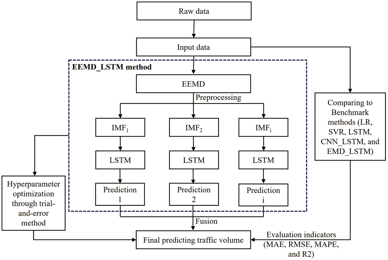
Figure 2: Diagram of the methods developed for traffic volume prediction

2.4 Hyperparameter Optimization and Benchmark Method Architecture

Before building the EEMD_LSTM model, it is necessary to choose a set of hyperparameters. These parameters include the lookback window, the number of neurons in the hidden layers, and the gradient descent optimizations. Hyperparameter optimization is a helpful approach to obtaining a fantastic method architecture. Nevertheless, there is no specific regulation for selecting these parameters. Hence, the trial-and-error process is the most reliable way to choose hyperparameters for each experiment.

A lookback window shows how many previous timesteps are used to forecast the next timestep. In this work, the value of the lookback window is 5, 15, 30, and 60 min.

The number of neurons in the hidden layers tremendously influences the final output. A few neurons in the hidden layers will lead to underfitting. Many neurons in the hidden layers will lead to overfitting. In this study, the number of hidden layers consists of 64, 128, and 256.

In addition, the gradient descent demonstrated that its performance is adequate for deep learning optimization [32]. To minimize the objective function, the gradient descent algorithm updates its parameters. In this work, we apply stochastic gradient descent (SGD), adaptive learning rate (AdaDelta), and adaptive moment estimation (ADAM) to obtain the best hyperparameter. First, the SGD applies one batch size per iteration through random choice. It also gets an update to move the redundant data.

θ=θ−η.∇θJ(θ,x(i),y(i))(10)

In Eq. (10), x(i) is the input data, y(i) is the labels, η is the learning rate, J(θ) is the objective function, and ∇θ is the objective function gradient.

Second, the AdaDelta moves the window of the gradient updates to improve the acceleration learning (i.e., converging to zero).

E[g2]t=ρ.E[g2]t−1+(1−ρ)gt2(11)

In Eq. (11), E[g2]t is the expected value of the accumulated gradient at time t, E[g2]t−1 is the expected value of the accumulated gradient at time t−1, ρ is the decay constant, and gt is the parameter gradient.

Third, the ADAM, an extension to stochastic gradient descent, estimates the average of the second moments of the gradients. It is helpful for big data with low memory space.

E[vt]=E[gt2].(1−βt2)+ζ(12)

In Eq. (12), E[vt] is the expected value of the exponential moving average at a timestep t, and E[gt2] is the true second moment.

To demonstrate the advantage of the proposed method, EEMD_LSTM is compared with others, such as LR, SVR, LSTM, CNN_LSTM, and EMD_LSTM. The LR method shows the relationship between independent and dependent variables. This model minimizes the residual sum of squares between the predicted and observed targets through a linear approximation. The SVR is a form of SVM for regression issues in the context of non-linear data. In this work, we set 15-minute lookback windows for those methods. Furthermore, the CNN_LSTM model uses convolution operations instead of internal matrix multiplications. In this study, the CNN_LSTM model consisted of two convolutional layers, two max-pooling layers, and one LSTM layer [15].

2.5 Evaluation Indicators

This study evaluates the prediction accuracy by MAE, RMSE, MAPE, and R2. Firstly, the MAE is a negatively oriented point. In other words, the smaller the value obtained, the better the model is. The MAE estimates the average absolute differences between forecast and actual data, as shown in the following:

MAE=1n∑i=1n|yi−y^i|(13)

The RMSE, the square root of the average squared differences between forecast and actual data, applies to the quadratic scoring rule.

RMSE=1n∑t=1n(yi−y^i)2(14)

In Eqs. (13)–(14), n is several data points, yi is observed values, and y^i is predicted values.

Thirdly, the MAPE, the mean absolute percentage of predicted errors, applies to the forecast error. The error is calculated as the actual value minus the forecast value.

MAPE=1n∑t=1n|At−FtAt|(15)

In Eq. (15), n presents several fitted points, At shows the actual value, and Ft shows the forecast value.

Finally, the R2 illustrates the percentage of the variance for the dependent variable, which is clarified by the independent variable. The equation of R2 is shown as follows:

R2=SSregressionSStotal(16)

In Eq. (16), SSregression presents the explained sum of squares, and SStotal presents the total sum of squares.

3  Empirical Results and Analysis

3.1 Experiment Data

The Busan metropolitan area has higher congestion due to heavy traffic. Therefore, the Munhyeon intersection was chosen as the research area, as shown in Fig. 3. For instance, the left graph plots an overview of the study area. The right graph shows the details of the Munhyeon intersection. In this study, extensive and multiple datasets need to be obtained. Nevertheless, we limited the traffic volume to 1 month at 5-min intervals. The automatic vehicle identification recorded the raw data from 01 February 2021 to 28 February 2021. The total number of traffic volume data is about 8023. We selected the first 18 days as the training set, two successive days as the validation set, and the last 8 days as the testing set. In this network, we use traffic volume for each 5-min interval as the input and the output.

Figure 3: Research area at Munhyeon intersection, Busan, Korea

The data are visualized in Table 1 through standard deviation (Std), mean, median, minimum (min), and maximum (max). We also create a summary of the set of data values, which is illustrated in Fig. 4. This can be seen in Table 1 and Fig. 4, where the distribution of traffic is generally stable and reaches high values due to the higher number of vehicles on weekdays compared with weekends.

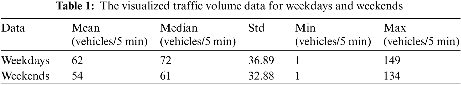
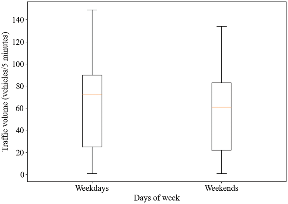
Figure 4: The box plot of traffic volume data for weekdays and weekends

This work executed experiments in the hardware environment: CPU intel i7-11700, Memory 16 GB, no GPU. The Tensorflow-based Keras is used in the software framework by adopting Python. Keras makes execution faster and reduces code repetition. In addition, the statistical time interval of these data is 5 min, and a total of 8023 pieces of traffic volume data are obtained. The trial-and-error method evaluated the algorithm during the experiment to optimize the hyperparameters and improve the prediction performance. These experiments are compared with the LR, SVR, LSTM, CNN_LSTM, and EMD_LSTM models. Therefore, the mean training time is about 340 s.

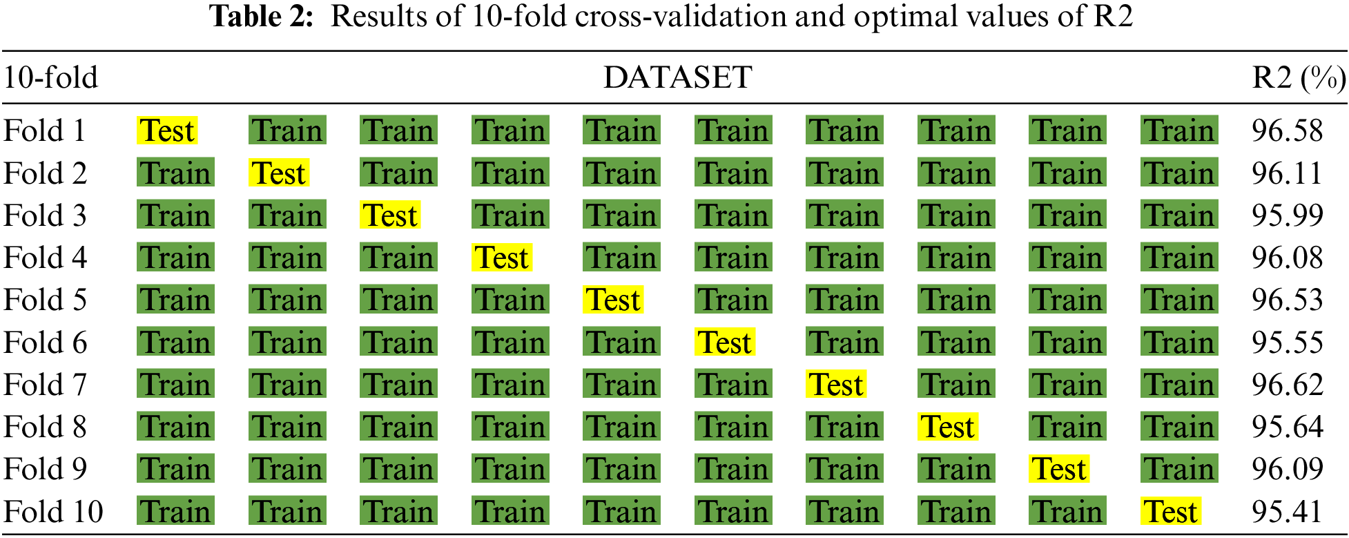
To evaluate the dataset’s quality in the context of the proposed method. We sorted the dataset by time and divided it into 10 subsets. Next, we executed a cross-validation technique on each of them. In other words, each subset has a chance to be a training dataset nine times and be a testing dataset once. The cross-validation results are shown in Table 2. These experiments indicate that our proposed model can forecast unseen data with a mean R2 value of 96.06%. Furthermore, these data are stable with a slight fluctuation range.

3.2 Decomposition Results

The decomposition results of EEMD are illustrated in Fig. 5. These results showed the characteristic fluctuation of different frequencies of traffic volume data. The order of the IMF showed the trending frequency from most significant to most minor. In particular, the high frequency of the IMF indicated an imbalance in short-term traffic volume. In contrast, the low frequency of the IMF showed instability characteristic of medium-term traffic volume. This process helps discover and learn more information and make predictions more accurate.

Figure 5: The EEMD results with nine intrinsic mode functions

3.3 Hyperparameter Optimization for Proposed Method

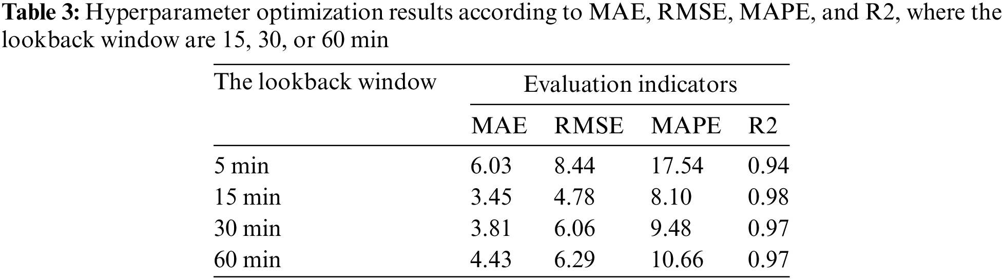
The lookback window’s value ranges from 1 to 12. Four experiments are conducted for each value of the lookback window using the proposed method. The lookback window consists of 1, 3, 6, and 12, corresponding to 5, 15, 30, and 60 min. The results of the lookback window optimization concerning MAE, RMSE, MAPE, and R2 for the proposed method are illustrated in Table 3. The proposed method can well characterize the rules of traffic volume when the lookback window is 15, 30, or 60 min. Nevertheless, when the lookback window is 5 min, the proposed model cannot accurately describe the rules of traffic volume. The proposed method with 15-min lookback windows achieved the lowest prediction error with the MAE, RMSE, and MAPE values of 3.45, 4.78, and 8.10, respectively. Similarly, the method with 15-min lookback windows achieved the highest prediction performance, with R2 values of 0.98. Compared to 60 and 15 min decreased the MAPE and RMSE values by 24% and 24%, respectively. Compared to 30 and 15 min decreased the MAPE and RMSE values by 14.5% and 21.2%, respectively. Therefore, the proposed method with 15-min lookback windows is suitable for forecasting traffic volume.

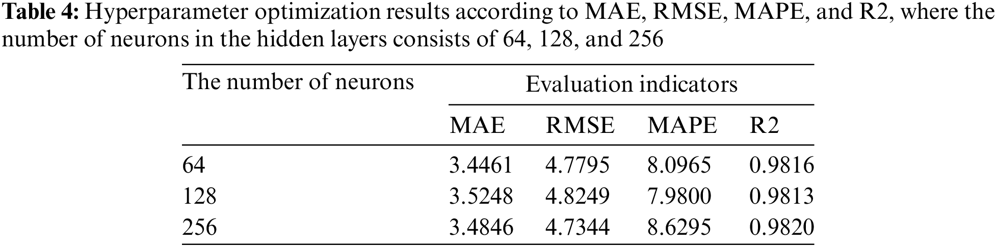
In addition, we conduct three experiments for each value of the number of neurons in the hidden layers. The number of neurons in the hidden layers consists of 64, 128, and 256. The results of the number of neurons in the hidden layers according to MAE, RMSE, MAPE, and R2 for the proposed method are shown in Table 4. The experimental results show little difference when changing the number of hidden layers. However, the proposed method with 256 hidden layers achieved the lowest RMSE (4.734) and the highest R2 (0.982). Therefore, the proposed method with 256 hidden layers is suitable for forecasting the traffic volume.

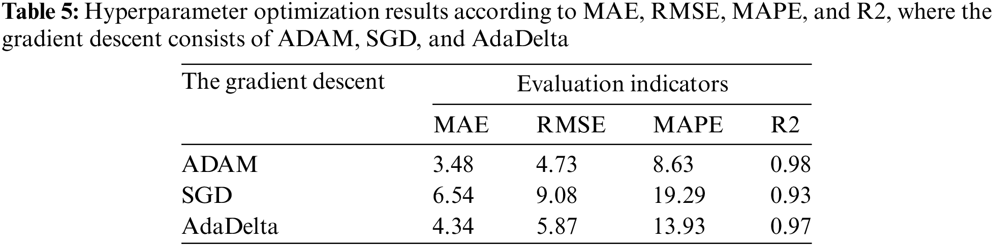
Finally, the proposed method conducts three experiments for each gradient descent. The gradient descent consists of ADAM, SGD, and AdaDelta. The gradient descent results for the proposed method according to MAE, RMSE, MAPE, and R2 are shown in Table 5. The proposed method with ADAM achieved the lowest prediction error with MAE, RMSE, and MAPE values of 3.48, 4.73, and 8.63, respectively. Similarly, the proposed method with ADAM achieved the highest prediction performance, with R2 values of 0.98. Compared to SGD, ADAM increased the R2 value by 5.2%. In addition, ADAM reduced by more than 55.3% in MAPE value compared to the SGD. Therefore, combining the proposed method with ADAM is suitable for forecasting traffic volume.

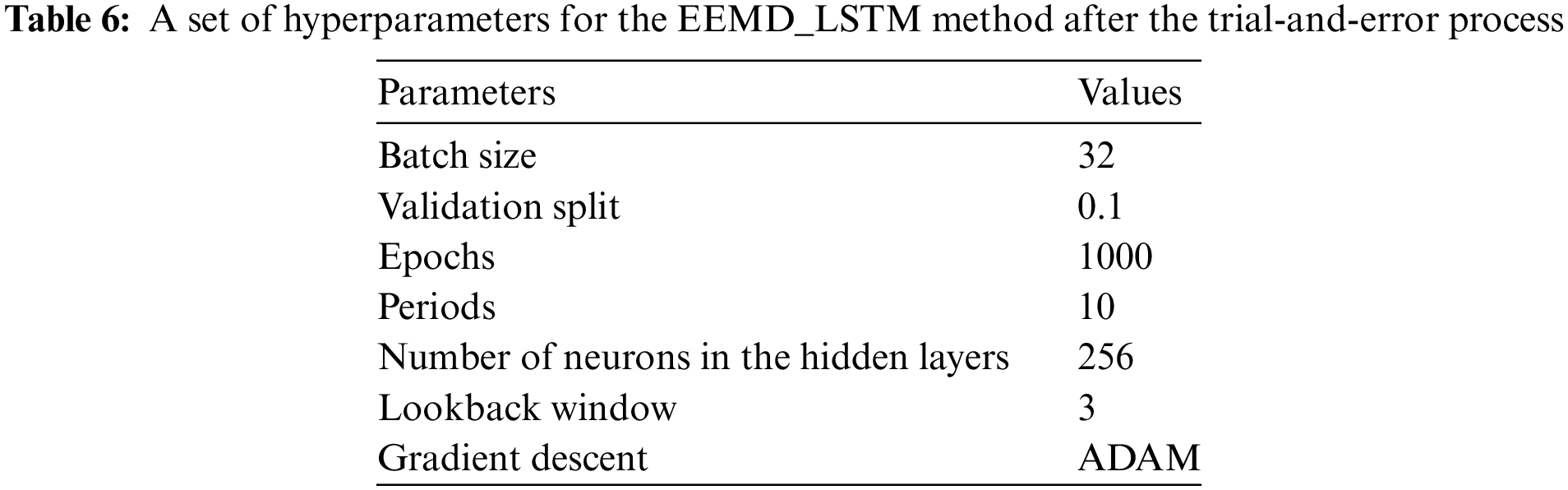
Therefore, a set of hyperparameters for the proposed method after the trial-and-error process is presented in Table 6.

3.4 Performance of Traffic Volume Prediction

To evaluate the performance of the proposed method, we used the MAE, RMSE, MAPE, and R2 to assess the predictive performance. The proposed method is compared with the LR, SVR, LSTM, CNN_LSTM, and EMD_LSTM models. The predictive performance is shown in Table 7. The comparison results regarding MAE, RMSE, MAPE, and R2 are shown in Figs. 6–7, respectively. The proposed model achieved the highest predictive performance with an R2 value of 0.98, followed by the EMD_LSTM and CNN_LSTM with 0.96 and 0.89, respectively. In other words, the proposed method clarified why the explained variance in the dependent variable achieved 98%, as mentioned above. Compared to CNN_LSTM, our proposed method increased the R2 value by 9.2%. Moreover, the proposed method obtained the most minor predictive error with the MAE, RMSE, and MAPE values of 3.48, 4.73, and 8.63, respectively. That means the proposed method decreased 61% of the MAE value, 61% of the RMSE value, and 67% of the MAPE value compared to CNN_LSTM. These systems consistently face significant computational demands, leading us to advocate for employing the EEMD_LSTM model as the suggested model to guarantee real-time performance and satisfactory positioning accuracy. The experiments confirm that the proposed method outperformed the other benchmark methods regarding the evaluation indicators.

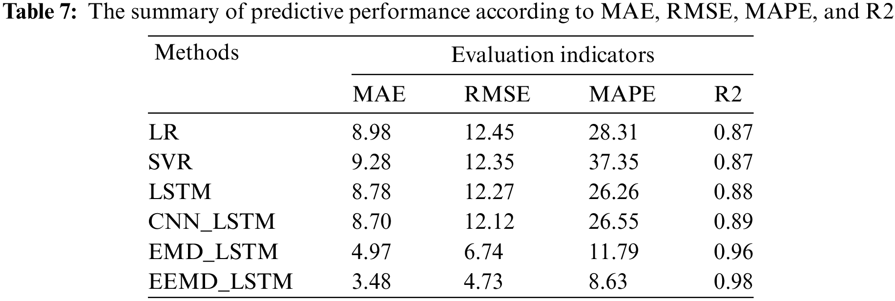
Figure 6: A comparison of the performance of the proposed method according to MAE, RMSE, and MAPE

Figure 7: A comparison of the performance of the proposed method according to R2

We also compare this work to other studies to determine its worth. For instance, our proposed method achieved the lowest prediction error with the RMSE value of 4.73, followed by [29] and [28] with 4.897 and 9.1, respectively. In addition, our proposed method achieved the lowest prediction error with the MAE value of 3.48, followed by [30] with 8.58. Thus, this study outperformed other studies regarding traffic volume prediction.

The testing data is used to verify the performance of the proposed model. The final prediction compared with the actual values is presented in Fig. 8. The visualization of the plot of actual and predicted values is illustrated in Fig. 8. In Fig. 9, the predicted values were close to the actual values for the proposed model. In Fig. 9, the scatter graph is almost linear, with an R2 of 0.9588. In other words, the proposed model explained 95.88% of the variance in the forecast value. Hence, the prediction model’s performance was suitable for the learning algorithm for the testing datasets. Thus, the proposed method achieves excellent performance in predicting traffic volume.

Figure 8: Comparison between the true and predicted values for the testing dataset

Figure 9: Scatter plot between the true value and predicted values for the testing dataset

To sum up, the experimental results show that the integration model that uses the EEMD and LSTM algorithms outstandingly enhances the prediction performance of the traffic volume. Furthermore, the proposed method obtained the highest prediction accuracy and the lowest prediction error compared to the benchmarks, such as the LR, SVR, LSTM, CNN_LSTM, and EMD_LSTM methods. The proposed model’s R2 value was 98% in the best-case scenario.

4  Conclusion

The enhanced ensemble-based deep learning method that used hyperparameter optimization-based EEMD and LSTM algorithms indicated superior predictive performance compared to the rest of the benchmark methods, namely LR, SVR, LSTM, CNN_LSTM, and EMD_LSTM paradigms regarding MAE, RMSE, MAPE, and R2 values. This paper selected the traffic volume data of Busan, Korea, for empirical validation. The experimental results demonstrated that the proposed model achieved better performance for traffic volume prediction. The main contribution of this study consisted of three characteristics. First, the proposed ensemble-based deep learning model was highly reliably forecasted by adopting the fusion of EEMD and LSTM algorithms. Second, the traffic volume data noise was decomposed and removed through the EEMD algorithm. Third, a set of optimal hyperparameters was suggested for the EEMD_LSTM method in the context of traffic volume prediction.

Furthermore, large and synthetic data can increase the efficiency of the predictive model. Due to the difficulty of data collection, synthetic data were not considered, and the dataset size needed to be more significant. We also concentrated on changing the hyperparameters for our proposed method. In addition, we only considered a specific location instead of the entire network. To further our research, we plan to focus on the following three aspects: (1) the real-time synthetic traffic data (e.g., speed, traffic volume, weather, and road condition) will be considered; (2) the data will be collected for about 7 months; (3) we will focus on improving the traffic prediction by strengthening the optimization of data preprocessing; (4) we will try to find better hybrid deep learning algorithms with spatial transmission characteristics; and (5) we will also compare with various algorithms to demonstrate the effectiveness of the proposed method. After making some developments to the algorithm, we will apply the proposed model for prediction in the context of urban networks.

Acknowledgement: Not applicable.

Funding Statement: The authors received no specific funding for this study.

Author Contributions: The authors confirm contribution to the paper as follows: study conception and design: Duy Tran Quang, Huy Q. Tran; data collection: Duy Tran Quang; analysis and interpretation of results: Duy Tran Quang, Huy Q. Tran; draft manuscript preparation: Duy Tran Quang, Minh Nguyen Van. All authors reviewed the results and approved the final version of the manuscript.

Availability of Data and Materials: Not applicable.

Conflicts of Interest: The authors declare that they have no conflicts of interest to report regarding the present study.

References

1. J. H. Ko, Seoul’s Transportation Demand Management Policy. Seoul, Korea: The Seoul Institute. Accessed: Jun. 24, 2015. [Online]. Available: https://www.seoulsolution.kr/en/content/seoul%E2%80%99s-transportation-demand-management-policy-general. [Google Scholar]

2. E. I. Vlahogianni, M. G. Karlaftis, and J. C. Golias, “Short-term traffic forecasting: Where we are and where we’re going,” Transp. Res. C: Emerg. Technol., vol. 43, pp. 3–19, Jun. 2014. doi: 10.1016/j.trc.2014.01.005. [Google Scholar] [CrossRef]

3. A. Richter, M. O. Lowner, R. Ebendt, and M. Scholz, “Towards an integrated urban development considering novel intelligent transportation systems: Urban development considering novel transport,” Technol. Forecast. Soc. Change., vol. 155, pp. 119970, Jun. 2020. doi: 10.1016/j.techfore.2020.119970. [Google Scholar] [CrossRef]

4. Y. Gu, W. Lu, L. Qin, M. Li, and Z. Shao, “Short-term prediction of lane-level traffic speeds: A fusion deep learning model,” Transp. Res. C: Emerg. Technol., vol. 106, pp. 1–16, Sep. 2019. doi: 10.1016/j.trc.2019.07.003. [Google Scholar] [CrossRef]

5. M. E. E. Alahi et al., “Integration of IoT-enabled technologies and artificial intelligence (AI) for smart city scenario: Recent advancements and future trends,” Sensors, vol. 23, no. 11, pp. 5206, May 2023. doi: 10.3390/s23115206. [Google Scholar] [PubMed] [CrossRef]

6. Z. H. Mir and F. Filali, “An adaptive Kalman filter based traffic prediction algorithm for urban road network,” in Proc. 12th Int. Conf. Inno. Inf. Techno. (IIT), Al Ain, United Arab Emirates, Nov. 28-30, 2016, pp. 1–6. [Google Scholar]

7. A. Emami, M. Sarvi, and S. A. Bagloee, “Using Kalman filter algorithm for short-term traffic flow prediction in a connected vehicle environment,” J. Mod. Transp., vol. 27, no. 3, pp. 222–232, Jul. 2019. doi: 10.1007/s40534-019-0193-2. [Google Scholar] [CrossRef]

8. J. Lee, B. Hong, K. Lee, and Y. J. Jang, “A prediction model of traffic congestion using weather data,” in Proc. IEEE Int. Conf. on Data Sci. and Data Intens. Syst., Sydney, Australia, Dec. 11–13, 2015, pp. 81–88. [Google Scholar]

9. S. Cheng, F. Lu, P. Peng, and S. Wu, “Short-term traffic forecasting: An adaptive ST-KNN model that considers spatial heterogeneity,” Comput. Environ. Urban Syst., vol. 71, no. 1, pp. 186–198, May 2018. doi: 10.1016/j.compenvurbsys.2018.05.009. [Google Scholar] [CrossRef]

10. F. Ahn, E. Ko, and E. Y. Kim, “Highway traffic flow prediction using support vector regression and Bayesian classifier,” in Proc. IEEE Int. Conf. Big Data Smart Comput., New York, USA, Jan. 18, 2016, pp. 239–244. [Google Scholar]

11. M. A. Haq, “SMOTEDNN: A novel model for air pollution forecasting and AQI classification,” Comput. Mater. Contin., vol. 71, no. 1, pp. 1403–1425, Nov. 2022. doi: 10.32604/cmc.2022.021968. [Google Scholar] [PubMed] [CrossRef]

12. K. Kumar, M. Parida, and V. K. Katiyar, “Short term traffic flow prediction for a non urban highway using artificial neural network,” Procedia Soc. Behav. Sci., vol. 104, no. 2, pp. 755–764, Dec. 2013. doi: 10.1016/j.sbspro.2013.11.170. [Google Scholar] [CrossRef]

13. B. Sharma, S. Kumar, P. Tiwari, P. Yadav, and M. I. Nezhurina, “ANN based short-term traffic flow forecasting in undivided two lane highway,” J. Big Data, vol. 5, no. 48, pp. 991–1007, Dec. 2018. doi: 10.1186/s40537-018-0157-0. [Google Scholar] [CrossRef]

14. W. Zhang, Y. Yu, Y. Qi, F. Shu, and Y. Wang, “Short-term traffic flow prediction based on spatio-temporal analysis and CNN deep learning,” Transportmetrica A: Transp. Sci., vol. 15, no. 2, pp. 1688–1711, Jul. 2019. doi: 10.1080/23249935.2019.1637966. [Google Scholar] [CrossRef]

15. Q. D. Tran and S. H. Bae, “A hybrid deep convolutional neural network approach for predicting the traffic congestion index,” Promet-Traffic & Transportation, vol. 33, no. 3, pp. 373–385, May 2021. doi: 10.7307/ptt.v33i3.3657. [Google Scholar] [CrossRef]

16. Q. Liu, B. Wang, and Y. Zhu, “Short-term traffic speed forecasting based on attention convolutional neural network for arterials,” Comput.-Aided Civ. Infrastruct. Eng., vol. 33, no. 11, pp. 999–1016, Sep. 2018. doi: 10.1111/mice.12417. [Google Scholar] [CrossRef]

17. S. Maher and P. Biswajee, “Severity prediction of traffic accidents with recurrent neural networks,” Appl. Sci., vol. 7, no. 6, pp. 476–486, Apr. 2017. doi: 10.3390/app7060476. [Google Scholar] [CrossRef]

18. A. Crivellari and E. Beinat, “Forecasting spatially-distributed urban traffic volumes via multi-target LSTM-based neural network regressor,” Math., vol. 8, no. 12, pp. 2233, Dec. 2020. doi: 10.3390/math8122233. [Google Scholar] [CrossRef]

19. M. A. Haq and M. A. R. Khan, “DNNBoT: Deep neural network-based botnet detection and classification,” Comput. Mater. Contin., vol. 71, no. 1, pp. 1729–1750, Aug. 2022. doi: 10.32604/cmc.2022.020938. [Google Scholar] [PubMed] [CrossRef]

20. B. H. Shekar and G. Dagnew, “Grid search-based hyperparameter tuning and classification of microarray cancer data,” in Proc. the 2019 Second Int. Conf. Adv. Comput. Commun. Paradigms (ICACCP), Gangtok, India, Feb. 25–28, 2019, pp. 1–8. [Google Scholar]

21. R. Andonie and A. C. Florea, “Weighted random search for CNN hyperparameter optimization,” Int. J. Comput. Commun. Control., vol. 15, no. 2, pp. 3868, Mar. 2020. doi: 10.15837/ijccc.2020.2.3868. [Google Scholar] [CrossRef]

22. C. Luo et al., “Short-term traffic flow prediction based on least square support vector machine with hybrid optimization algorithm,” Neural Process. Lett., vol. 50, no. 3, pp. 2305–2322, Mar. 2019. doi: 10.1007/s11063-019-09994-8. [Google Scholar] [CrossRef]

23. H. Peng et al., “Spatial temporal incidence dynamic graph neural networks for traffic flow forecasting,” Inf. Sci., vol. 521, no. 2, pp. 277–290, Jan. 2020. doi: 10.1016/j.ins.2020.01.043. [Google Scholar] [CrossRef]

24. H. Peng et al., “Spatial temporal incidence dynamic graph neural networks for traffic flow forecasting,” Inf. Sci., vol. 521, no. 2, pp. 277–290, Jan. 2020. doi: 10.1016/j.ins.2020.01.043. [Google Scholar] [CrossRef]

25. Z. Wang, L. Zhang, and Z. Ding, “Hybrid time-aligned and context attention for time series prediction,” Knowl.-Based Syst., vol. 198, pp. 105937, Jun. 2020. doi: 10.1016/j.knosys.2020.105937. [Google Scholar] [CrossRef]

26. L. Kuang, C. Hua, J. Wu, Y. Yin, and H. H. Gao, “Traffic volume prediction based on multi-sources GPS trajectory data by temporal convolutional network,” Mob. Netw. Appl., vol. 25, no. 4, pp. 1405–1417, Feb. 2020. doi: 10.1007/s11036-019-01458-6. [Google Scholar] [CrossRef]

27. Y. Zheng, C. Dong, D. Dong, and S. Wang, “Traffic volume prediction: A fusion deep learning model considering spatial-temporal correlation,” Sustain., vol. 13, no. 9, pp. 10595, Sep. 2021. doi: 10.3390/su131910595. [Google Scholar] [CrossRef]

28. X. Chen et al., “Robust visual ship tracking with an ensemble framework via multi-view learning and wavelet filter,” Sensors, vol. 20, no. 3, pp. 932, Feb. 2020. doi: 10.3390/s20030932. [Google Scholar] [PubMed] [CrossRef]

29. Z. Xuan, S. Xie, and Q. Sun, “The empirical mode decomposition process of non-stationary signals,” in Proc. 2010 Int. Conf. on Measuring Technology and Mechatronics Automation, Changsha, China, Mar. 13–14, 2010, pp. 866–869. [Google Scholar]

30. X. Chen et al., “Anomaly detection and cleaning of highway elevation data from google earth using ensemble empirical mode decomposition,” J. Transp. Eng. A: Syst., vol. 144, no. 5, pp. 58–72, May 2018. doi: 10.1061/JTEPBS.0000138. [Google Scholar] [CrossRef]

31. M. Anul Haq, “CDLSTM: A novel model for climate change forecasting,” Comput. Mater. Contin., vol. 71, no. 2, pp. 2363–2381, Dec. 2022. doi: 10.32604/cmc.2022.023059. [Google Scholar] [PubMed] [CrossRef]

32. E. M. Dogo, O. J. Afolabi, N. I. Nwulu, B. Twala, and C. O. Aigbavboa, “A comparative analysis of gradient descent-based optimization algorithms on convolutional neural networks,” in Proc. 2018 Int. Conf. on Comput. Tech., Electron. and Mech. Syst. (CTEMS), Belgaum, India, Dec. 21–22, 2018, pp. 92–99. [Google Scholar]