Double DQN Method For Botnet Traffic Detection System

1  Introduction

With the rapid development of technology, the internet environment has become increasingly severe. Starting from Mixter’s introduction of Distributed Denial-of-Service (DDoS) in the “TFN” toolkit on Internet Relay Chat (IRC) in 1999, which released the first botnet plugin [1], to today’s everyday use of HTTPS and Peer-to-Peer (P2P) as invasion methods for botnet traffic [2], the threat posed by a botnet to hosts and websites is becoming more significant. Attackers implant malicious software or viruses into computers or Internet of Things (IoT) devices through various means, such as launching DDoS attacks, propagating malware, phishing, and click fraud against critical targets, invading and infecting target hosts, making them “botnet nodes,” and then using these nodes to continue attacking other targets, forming large and small botnet families. Users are unaware that their hosts have been infected. After constructing a botnet, attackers simultaneously send large amounts of data packets or requests from target servers to the infected “botnet” nodes, occupying the server’s processing capacity and bandwidth resources, thereby preventing normal users from accessing the server and forcing the server to shut down due to resource exhaustion.

In June and July 2022, China experienced 26,000 cases of cybersecurity breaches events [3]. According to Kaspersky’s 2022 security report, China accounted for 17.70% of the world’s Trojan and botnet invasions [4]. In addition, in March 2022, Toyota suffered a system shutdown due to supplier receipt of botnet software attacks, while in May, its Asian subsidiary, Nikkei Group, located in Singapore, was also attacked by botnet software. That same month, SpiceJet, an Indian airline, was also assaulted by botnet software, resulting in hundreds of passengers being stranded at the country’s airports. Some super-large botnet families contain tens of thousands of infected hosts, while others are small botnet families with less than one hundred infected hosts [5]. Due to the P2P end-to-end data transmission mode, it is difficult to determine the location of the controller’s host in botnet tracing, so the only option is to continuously improve their detection capabilities to prevent hosts from being infected by a botnet. This problem poses a significant threat to global cybersecurity.

In the early stages of internet development, detecting IRC botnets was relatively easy due to the open nature of the IRC protocol. The earliest detection methods were based on traffic filtering rules such as port, protocol, and source address. Still, this method could only detect known attack traffic and not new types of attacks, such as using P2P protocols for decentralization and conducting large-scale distributed attacks. Therefore, in a botnet constructed with it, botnet hosts communicate through a centralized server and a P2P network for connection and communication. Use to detect this type of botnet traffic, special techniques are required. One standard method is based on statistical analysis and machine learning algorithms to analyze and identify traffic through feature extraction and classification algorithms. This method can detect P2P botnet traffic and detect new unknown attacks.

As technology continues to develop, detection methods and capabilities are constantly improving. Modern detection methods include feature analysis, data mining, behavior analysis, machine learning, deep learning, and other technologies. This article combines feature engineering and extraction from machine learning classifiers, high-dimensional deep learning inputs, and real-time reinforcement learning capabilities to create a detection model for botnet traffic. By identifying and classifying features of the dataset, convenient features are selected and trained using the detection model to recognize all types of attacks and detect botnet traffic.

2  Structure

As botnet technology continues to evolve, detection techniques are constantly improving based on the characteristics of botnet traffic. During the early days of IRC chat rooms, Zeidanloo et al. developed a signature-based detection method by matching known malicious code samples to identify infected botnets in response to attack methods such as remote execution vulnerabilities and password cracking. Additionally, computer system behavior analysis, such as network traffic and process behavior, can detect abnormal behavior but may generate some false positives [6]. Zhao et al. grouped data packets with the same properties of the IP five-tuple (source IP address, destination IP address, source port number, destination port number, protocol identifier) into a data stream using TCP/UDP protocols, then partitioned the data stream using time windows to achieve botnet detection [7]. After conducting a feature importance analysis, Hijawi et al. detected Android botnet URL feature sets, resulting in a significant interception of botnet traffic packets [8].

As machine learning began to gain traction in various fields, Joshi proposed combining support vector machines (SVM) and random forest classifier (RFC) to classify the N-BaIoT dataset, effectively separating abnormal behavior traffic from regular traffic. However, accuracy still needs improvement [9]. Afterward, numerous teams and researchers utilized various machine learning algorithms for detection, such as decision trees, K-Nearest Neighbor (KNN), multi-layer perceptron (MLP), naive Bayes, random forest, SVM, and data sets based on each time window, which achieved high accuracy rates through gradient boosting for botnet detection. Their models used these datasets and produced high accuracy rates [10–18].

With the rise of deep learning, neural networks that have evolved from MLP have gradually become the foundation for constructing complex models. Models such as Recurrent Neural Networks (RNNs), Convolutional Neural Networks (CNNs), and Long Short-Term Memory (LSTM) are built upon this foundation. Torres et al. proposed using RNNs and achieved an astonishing 98% accuracy in detecting a small amount of data samples using 5-fold cross-validation [19]. Pektas et al. employed Deep Neural Networks (DNNs) to model network traffic and detect botnet traffic [20]. Hussain et al. utilized the ResNet-18 residual network to detect scanning activities and DDoS attacks during the zero-day phase of botnets [21]. Chen addressed network degradation issues using the residual spatiotemporal network and designed the Res-1DCNN-LSTM model by combining LSTM and CNN to detect botnet traffic data samples [22]. Qi combined CNN and LSTM, merging spatial and temporal features for identification. They improved accuracy by using small convolutional kernels and the GELU activation function [23].

Furthermore, they augmented and enhanced the dataset using Generative Adversarial Networks (GANs). They employed transfer learning to utilize the discriminator as a novel botnet detector, enabling excellent performance even with imbalanced datasets. Qi utilized the CFR algorithm for feature selection and employed a model structure that combines BiGRU and CNN to enhance accuracy and computational efficiency. The residual module and ELU activation function were referenced to strengthen the model’s ability to extract low-frequency attack features. An attention mechanism was introduced to handle essential features. This detection method achieved a multi-classification accuracy of 99.77% and 99.24% on the CIC-IDS2017 and TON_IoT datasets, with binary classification accuracies of 99.82% and 99.62% [24]. Xue et al. integrated deep learning with the Internet of Things (IoT) and designed a bidirectional LSTM-RNN model to detect botnet activities in user IoT devices and networks [25].

In 2013, Volodymyr and the DeepMind team introduced the Deep Reinforcement Learning (DRL) concept. They combined the Q-learning algorithm of reinforcement learning with the high-dimensional nature of deep learning, resulting in the proposed DQN algorithm. In 2015, they demonstrated the capabilities of their model built using the DQN algorithm by surpassing some human players and achieving high scores in Atari games [26]. Building upon this work, the Hado team introduced the concept of DDQN, utilizing two neural networks to estimate Q-values and address the issue of overestimation [27]. Due to its real-time updating strategy, deep reinforcement learning has been extensively applied in fields such as autonomous driving and autopilot systems. Zuo et al. employed DDQN for object detection, enabling rapid identification of objects within a brief timeframe [28]. In network security, Wen utilized deep reinforcement learning to generate adversarial samples for evading JavaScript malware detection models, thereby evading malicious code for anti-virus purposes [29].

With the emergence of GANs, the approach to detection methods has shifted from passive defense to proactive offense. McDermott approached botnet detection from the perspective of GANs, generating samples to continually challenge the detector and provide better guidance, thereby enhancing the model’s ability to detect unfamiliar samples [30]. This approach has paved the way for subsequent botnet detection. Venturi et al. created an adversarial dataset using GANs to evade traditional machine learning detectors. Experimental results showed that this dataset had a detection evasion rate of 84% in traditional detectors like RF and SVM [31].

Not only that, but the successful combination of DQN and GAN has elevated botnet detection to new heights. Wu et al. proposed a framework based on deep reinforcement learning that effectively generates malicious traffic by automatically adding perturbations to samples to deceive detection models. Experimental results showed a significant improvement in the evasion rate while helping the detection model identify vulnerabilities and enhance its robustness [32]. The Apruzzese team introduced a deep reinforcement learning mechanism framework that protects botnet detectors from adversarial attacks. It was validated on various machine learning algorithms and public datasets, demonstrating significant improvements compared to existing techniques [33]. The Randhawa team presented a deep reinforcement learning (DRL) GAN model called RELEVAGAN. DRL is utilized to automatically modify the content of the generator, allowing it to bypass the discriminator’s detection. This enables the discriminator to undergo more complex training, significantly enhancing its detection capability compared to models without DRL [34].

3  Methodology

This paper proposes an OneR-DDQN model constructed using the machine learning OneR classifier and the deep reinforcement learning DDQN algorithm. The aim is to maintain high predictive capabilities for different botnet datasets. The entire process is divided into four steps: Merging and preprocessing the datasets, conducting feature engineering with machine learning to select relevant features, building the DDQN model, comparison experiments with the built DDQN model and the DQN model to compare the performance of the two algorithms under different datasets, to using the existing deep learning LSTM detection model as an objective model judging reference. This paper also explores the impact of feature engineering without using the OneR classifier during model training. The experimental procedure and model framework are illustrated in Fig. 1.

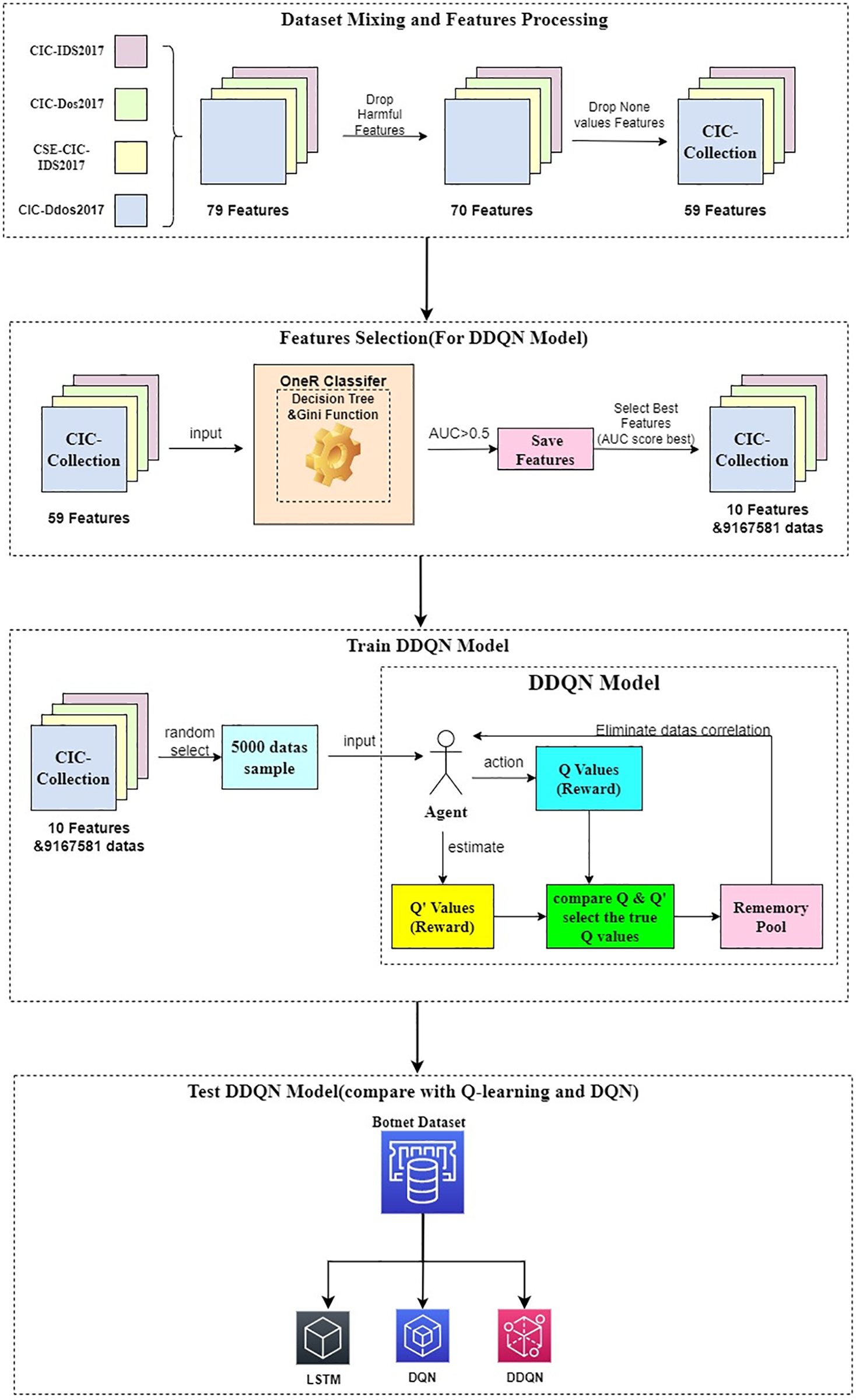
Figure 1: Flow diagram of botnet traffic detection based on DDQN algorithm

3.1 Dataset

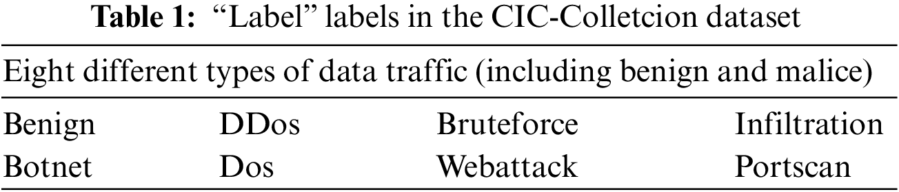
The datasets used in this study are from the CIC-IDS series provided by the Canadian Institute for Cybersecurity. The datasets include CIC-IDS2017, CIC-Dos2017, CSE-CIC-IDS2018, and CIC-DDos2019. The NumPy library was employed in this paper to merge labels with the same label values and filter out certain data samples. The resulting merged dataset is referred to as the CIC-Collection, and the corresponding label values obtained are presented in Table 1.

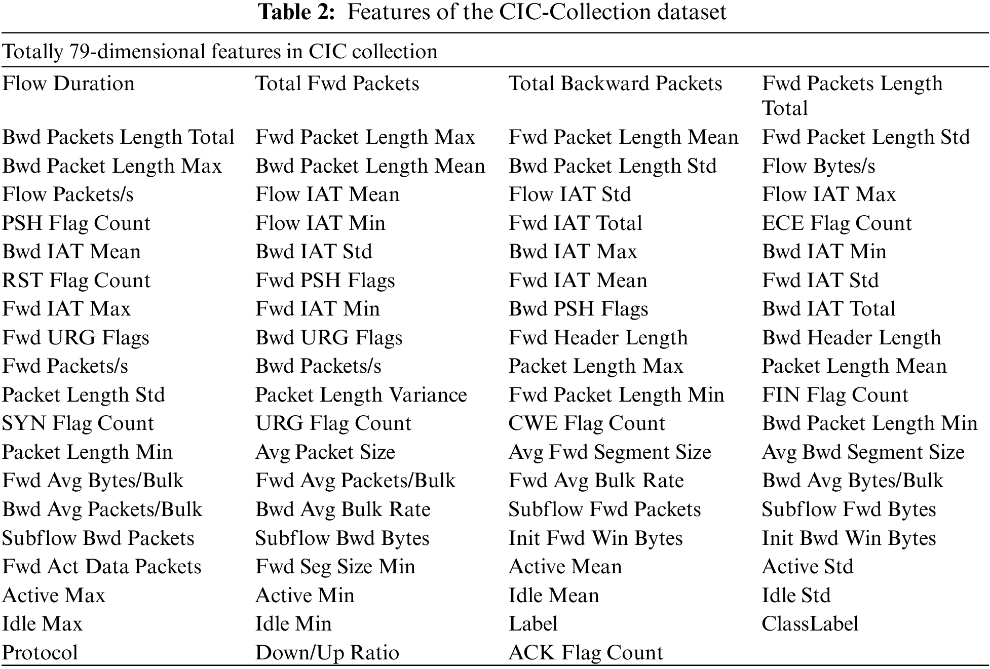
Each label is associated with the features from the four datasets. By using the Pandas library for data reading, there are a total of 9,167,581 records with 79-dimensional features as shown in Table 2.

However, not all features are relevant or informative. The dataset contains certain features completely irrelevant for prediction, referred to as pollution features, and need to be discarded. Following the ranking of feature pollution severity, this paper utilized the drop function to remove nine features, as shown in Table 3.

There are also some features, such as Active Std and Idle Std, that can affect the dataset. However, after data batching on the smaller dataset, the degree of feature pollution is not significant or noticeable, so these features are retained.

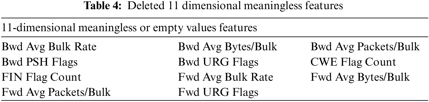
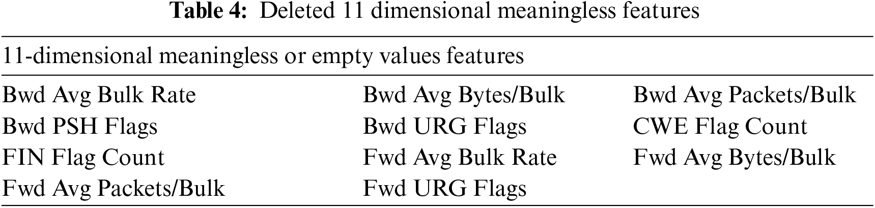
During the process of identifying polluted features, this study discovered 11 features with a predictive capacity of zero. These features have no meaningful value in any classification model, and some even have None as their feature values. For these features, the drop function was also used to discard them, as shown in Table 4.

Through the three steps described above, this study obtained a clean sample dataset (CIC-Collection) of four datasets. The dataset contains detailed labels for personal attacks and corresponding broader attack categories. There are no None values, and no duplicate samples exist. The dataset comprises 9,167,581 records, with each record having 59-dimensional features. The dataset is stored in the Parquet file format.

Like CSV files, Parquet files also can be directly read through Python’s built-in library. However, Parquet files offer smaller compressed storage space and more efficient reading than CSV files. The Pyarrow library is a built-in Python library specifically designed for reading datasets, which can read CSV files, parquet files, and other datasets files.

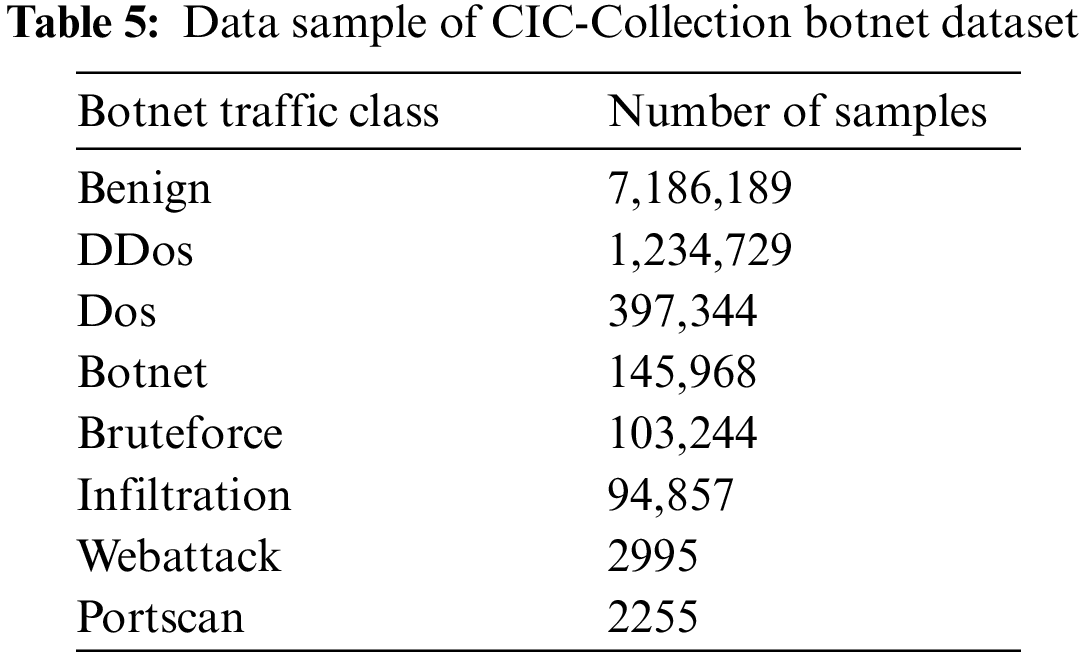
An example of the data samples in the dataset is presented in Table 5, by Pyarrow library reading.

The process of mixing and preprocessing specific datasets is shown in Fig. 2.

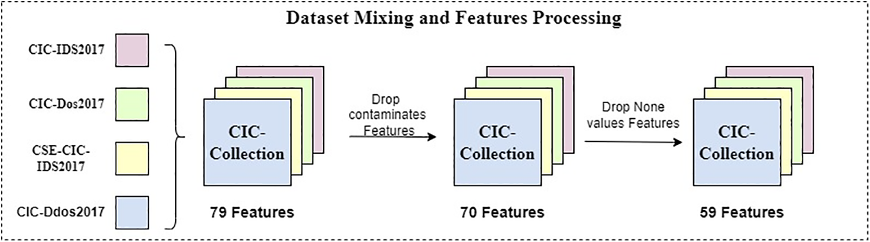
Figure 2: Dataset mixing and features preprocessing

3.2 Feature Selection of OneR Classifiers

After obtaining the preprocessed dataset, selecting the most suitable features for training the detection model is necessary. Otherwise, the model’s performance may vary depending on the features used. If the selected features are irrelevant to the detection task, training the model using these features will naturally result in poor detection capability. Therefore, this study introduces the OneR algorithm, which is a machine learning technique, for feature selection.

The OneR algorithm was initially proposed by Holte in 1993 and has since been applied in various fields, including medical diagnosis, credit scoring, and text classification. The OneR classifier is a simple yet effective algorithm for constructing rule-based classification models. It works by selecting a single feature from the dataset and determining the most frequently occurring class for each unique value of that feature. This process generates a set of rules that can be used to predict the class based on the feature values of new instances [35].

The OneR algorithm is highly efficient in computation and suitable for large datasets with many features. Additionally, it can provide valuable insights into the most significant features of a specific classification problem, aiding in feature selection and interpretation.

The algorithm of the OneR classifier is as follows:

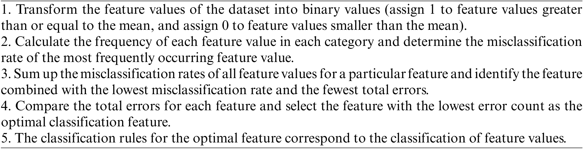
Before performing the classification operation with the OneR classifier, due to the OneR classifier’s inability to judge features of some string types, using string for feature classification makes OneR make counterproductive judgments. It is necessary to discard certain features that cannot be used for classification, such as features of “type” type. After this preprocessing step, the dataset is reduced to 44 dimensions. It reduces feature dimensions and noise and allows the OneR classifier to focus on making reasonable judgments about the remaining features. At the same time, due to the dataset having 9.17 million pieces of data, it is suitable for the OneR classifier, which processes a large number of data samples. Using the OneR classifier can effectively avoid overfitting compared to other classifiers.

Then, the remaining features are input into the OneR classifier, which has a machine-learning decision tree classifier at its core. The decision tree has a depth of 1 layer and uses the Gini coefficient.

Next, the dataset is divided into a training set and a testing set at 80% and 20% ratios, allowing the OneR classifier to complete the judgment after a brief training session. After fitting the training set, predictions are made on both the testing and training sets using the prediction function. The evaluation metrics are then calculated by comparing the predicted results with the accurate labels. If the metric evaluation value is more significant than 0.5, the feature name, metric value, and prediction result of that feature are saved. These values are stored in a list and converted into a data frame. The metric evaluation value, specifically the roc_auc_score, is calculated directly using the metrics method from the sklearn library.

Based on the metric evaluation value (roc_auc_score) greater than 0.5, features with significant discriminatory power are selected. The average prediction results on the testing and training sets are computed for these valuable features, resulting in an overall prediction result vector. The ROC curve parameters are then calculated based on the overall prediction results and proper training set labels.

ROC curve (receiver operating characteristic curve) is a graph showing the performance of a classification model at all classification thresholds. The calculation method for the ROC curve is as follows:

ROC=TPR−FPR(1)

TPR (True Positive Rate) represents the probability of correct predictions, and FPR (False Positive Rate) represents the probability of incorrect predictions. The area under the ROC curve (AUC score) is used as a widely recognized standard for evaluating the overall performance of classifiers. The AUC value ranges from 0 to 1, with higher values indicating better performance. The random selection benchmark is set at an AUC score of 0.5, with features having an AUC score greater than 0.5 considered more informative for classification. The flowchart of the OneR classifier process is depicted in Fig. 3.

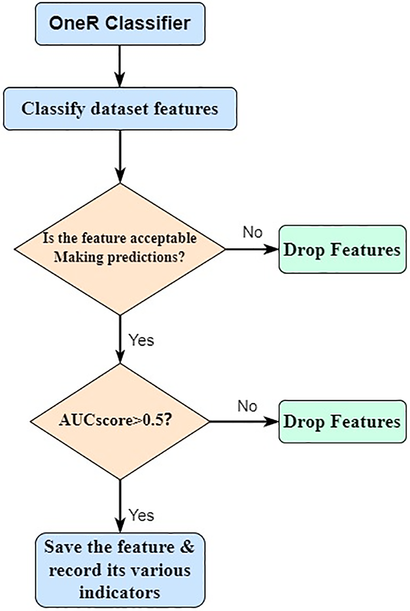
Figure 3: The working principle of feature selection for OneR classifier

After constructing the OneR classifier, the study proceeds by inputting the samples, excluding Benign, into the classifier for each of the seven attack methods. The ROC curves are then generated based on the best-performing feature for each attack, as shown in Fig. 4.

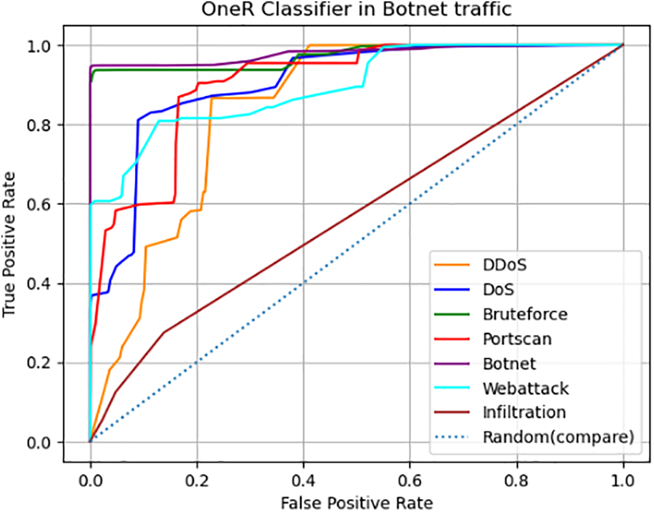
Figure 4: ROC curve of OneR classifier in botnet traffic

The OneR classifier performs perfect ROC curves in attacks such as Bruteforce and Botnet. It indicates its ability to accurately identify most samples in these attack categories without additional learning. However, its effectiveness diminishes when dealing with Infiltration attacks, as it exhibits no discerning capability. The study then proceeds to use the metrics class from the sklearn library to compute and obtain the top-ranked 2-dimensional features for each attack, resulting in 14 features, as shown in Table 6. From these features, the most effective ones are selected as inputs for the detection model.

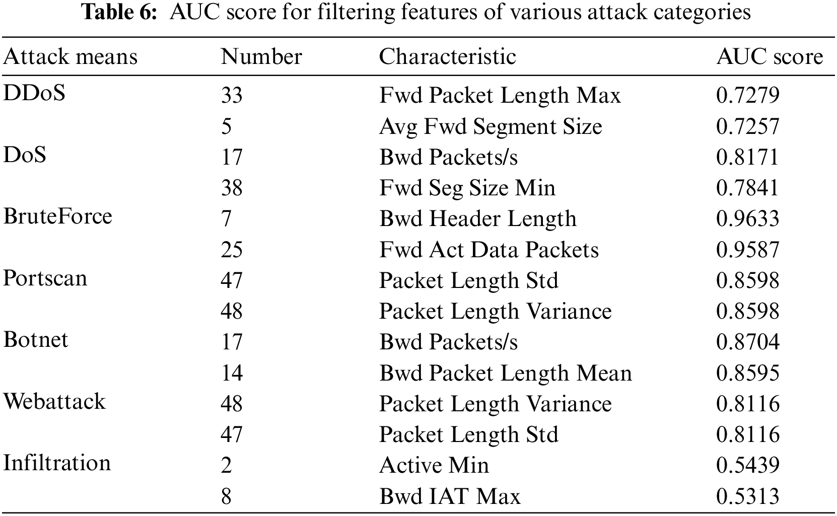
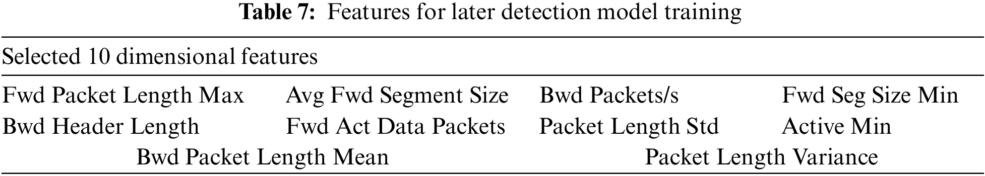
In the subsequent detection model training, feature selection is crucial in achieving high performance. Since features 17, 47, and 48 have appeared among the features the classifier selects, count them only once to avoid repeatedly adding the same features, which may result in varying numbers used in the model. Feature 8 (Bwd IAT Max) has shown poor performance. It may occupy a certain number of features but may not bring good judgment results. These four features will exclude. The other features not selected do not mean that Botnet traffic cannot be judged, but the ability to judge Botnet traffic is not so good compared to the selected 10-dimension feature. The remaining 10-dimensional features are chosen as the input for training the model as shown in Table 7.

The entire feature selection process illustrated in Fig. 5.

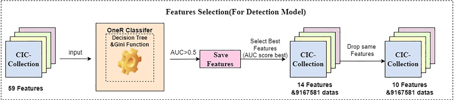
Figure 5: Feature selection

Now, the OneR classifier has completed feature selection, and these 10-dimensional features will be input into the detection model as input values. The detection model will learn how to judge whether the traffic belongs to Botnet traffic through these features through training and memory of neural network. Although unselected feature values may provide learning capabilities for the detection model, the directionality and detection capabilities provided by features classified by OneR will be more powerful.

3.3 DDQN Detection Model

From the Q value obtained from the earliest prediction results to record the feedback value to train the Q-learning algorithm of the model to the DQN algorithm using neural networks and constantly updating the target network to obtain the constantly updated Q value to the DDQN of double Q values set to reduce the excessive prediction of Q-values, the differences in the detection models of these three Reinforcement learning make the construction of their detection models more complicated.

Due to the extension of DDQN from DQN, an extension of Q-learning, this study constructs models based on Q-learning, DQN, and DDQN sequentially. Due to the inability of Q-learning to handle high-dimensional features (mentioned in Section 3.3.1), this article only compares the capabilities of the DQN model and the DDQN model. In addition, 9.16 million pieces of data are enormous and a burden for computers. Therefore, this article randomly selects 20,000 pieces of data from the data each time and divides them into training and testing sets according to 80% and 20% for the learning and training of the detection model. The DQN and DDQN models are trained using the same training set. Finally, the performance of these three detection models is compared using the same test set. In addition, to test the model’s adaptability to unfamiliar environments, we use different data sets to evaluate. In four original data sets, the original CIC-IDS2017 data set has more complex data. Hence, this data set poses a more significant challenge to the detection model than the other three. We input this data set into the model for detection to evaluate the model, For further comparative testing.

3.3.1 Q-learning Model

Q-learning is the foundational algorithm for both DQN and DDQN. It is a value-based reinforcement learning algorithm used to solve problems in Markov Decision Processes (MDP). In an MDP, an agent interacts with an environment over discrete time steps. At each time step, the agent observes the current state of the environment and takes action. The environment then transitions to a new state, giving the agent a reward signal. By estimating the value or utility of each state, agents can make decisions that maximize the long-term cumulative rewards. Furthermore, MDP helps agents learn to make optimal decisions based on the given rewards and transition probabilities, and Q-learning follows the reward mechanism of it. The ultimate goal of Q-learning is to choose the optimal policy in each prediction, which maximizes the accumulation of Q-values and rewards. At each step, Q-learning obtains a state-action value function, denoted as Q(st,at), representing the expected cumulative return when taking a specific action in a given state. The optimal decision sequence in the MDP can be derived by solving the Bellman equation, resulting in the Q(s,a) state-action value function as shown in Eq. (2).

Qπ(s,a)=Eπ[rt+1+γrt+2+γ2rt+3+…|at=a,st=s](2)

In the context of the given equation, “rt+1+γrt+2+γ2rt+3+…” represents the total discounted reward starting from time step t. γ is the discount factor, which ranges between 0 and 1. A higher value of γ indicates a greater consideration of the long-term value of future states, while a lower value of γ focuses more on immediate rewards. Therefore, a higher γ value is chosen in the early stages to encourage the model to explore longer-term rewards. As the number of epochs increases, γ gradually decreases, leading to a gradual decrease in the model’s learning ability and eventual convergence. Based on this, Q-value formula can be derived as shown in Eq. (3).

Q(st,at)←Q(st,at)+α[r+γ maxa′⁡Q(st′,at′)−Q(st,at)](3)

In the equation, “st” represents the current state, “at” represents the action taken in the current state, “r” represents the immediate reward obtained after taking the action at, “s′” represents the next state reached after taking the action, and “α” is the learning rate parameter. This calculation formula uses temporal difference learning to update the Q-value. It selects the maximum Q(st′,at′) from the next state “s′” and multiplies it by “γ,” then adds the actual reward value “r” to obtain the final true value of Q(st,at).

Due to the large sample size and excessive number of features in the dataset, the Q-learning algorithm only focuses on the interaction between one or two features and the environment. Once the dimensions expand significantly, the Q-learning algorithm will likely experience a “Curse of Dimensionality” phenomenon, which can lead to abysmal results. So in this experiment, Q-learning is not utilized to build a Q-learning model due to its inability to handle high-dimensional feature inputs. However, Q-learning can learn the optimal policy through exploration without prior knowledge of the environment, which is what we need. Subsequently, DQN and DDQN are extensions and enhancements based on Q-learning.

3.3.2 DQN Model

In order to overcome the problem of the “Curse of Dimensionality,” experts in the field of Reinforcement learning integrate the advantages of deep learning into reinforcement learning. First, the deep learning neural network can help reinforcement learning better learn many complex problems. Second, through the neural network, reinforcement learning will also have more acceptable and learning feature dimensions, thus solving the problem of the “Curse of Dimensionality.” The DQN is the first algorithm in deep reinforcement learning and an extension of the Q-learning algorithm in the context of deep learning. It is a model that combines reinforcement learning and deep learning successfully. DQN utilizes neural networks to approximate the Q-value function, enabling learning in high-dimensional and complex state spaces while possessing some generalization capability. In addition, DQN also advanced the Q table into a Q network, which can load more sample content for intelligent agents to learn.

The network architecture used in DQN consists of three convolutional layers followed by two fully connected layers. The Q-value function is denoted as Q(s,a;θ), and updating the network essentially means updating its weight parameters, denoted as θ. Once θ is determined, the neural network’s parameters are also determined. Compared to the Q-table used in Q-learning, the Q-network contains more information and useful insights for making judgments.

The ε-greedy strategy is vital to the exploration-exploitation trade-off in deep reinforcement learning. The ε-greedy strategy balances exploring new actions and exploiting the current knowledge to maximize cumulative rewards. Initially, when the agent has limited knowledge about the environment, exploration is given more weight (higher ε value) to ensure a broader exploration of the state-action space. As the agent learns and accumulates more experiences, the exploitation component becomes more dominant (lower ε value) to exploit the learned Q-values and maximize rewards. The DQN algorithm in this paper utilizes the ε-greedy strategy, which differs from the greedy approach that always selects the action with the maximum value function, denoted as at=maxaQ(st,a;θ). It incorporates a parameter ε, where the algorithm randomly selects an action at=maxaQ(st,a;θ) from all possible actions with a probability of ε. with a probability of 1 – ε, it selects at=maxaQ(st,a;θ) based on the maximum value from the Q-network. As the number of iterations increases, ε decreases, causing the model to increasingly favor selecting actions based on the maximum value from the Q-network. This approach ensures both the exploration characteristic of reinforcement learning and the utilization of the maximum value function.

The DQN algorithm starts by providing an environment state s to the agent, who then utilizes the value function network to obtain all Q(s,a) values associated with state s. The agent decides by employing the ε-greedy strategy to select an action a. The environment responds to the action by providing a reward value “r” and the following environment state s’. This completes one epoch. The parameters of the value function network are then updated based on the reward value “r,” and the process proceeds to the next epoch. This cycle continues until a converged value function network is trained, concluding the loop. The workings of one epoch are depicted in Fig. 6.

Figure 6: DQN neural network structure

At the algorithm level, DQN extends the Q-learning algorithm. However, since DQN approximates the Q-values using a neural network, determining the “θ” weights of the neural network becomes crucial in the entire process. In this study, the gradient descent algorithm is employed to minimize the loss function, continuously adjusting the θ weights. The algorithm for the loss function is depicted as Eq. (4).

Li(θi)=E(s,a,r,s′)∼U(D)[(r+γmaxa′⁡Q(s′,a′;θi−)−Q(s,a;θi))2](4)

In the equation, θi represents the parameters of the Q-network neural network at the i-th iteration, and θi− represents the parameters of the target neural network at the i-th iteration. Q(s,a;θi) represents the Q-value function for taking action a in the current network state, which is used to evaluate the Q-value generated by the current state-action pair. Q(s′,a′;θi−)represents the output of the target network. By introducing the target network, the target Q-values remain unchanged for a certain period of time, reducing the correlation between the current Q-values and the target Q-values to some extent, thereby improving the stability of the algorithm. The gradient descent is then performed on θ, as shown in Eq. (5).

∂Li(θi)∂θi=E(s,a,r,s′)∼U(D)[(r+γmaxa′⁡Q(s′,a′;θi−)−Q(s,a;θi))∇QiQ(s,a;θi)](5)

After every N iteration of gradient descent, the parameters of the current network are copied to the target network, which eventually outputs the converged Q-value function.

In the botnet traffic detection model, to facilitate agent learning, when the agent selects an action to classify the traffic type, it receives a reward value “r”. The reward function is defined as follows:

r={5,True−5,False−0.1,Not judged every 1 ms(6)

When the agent makes a correct selection, positive feedback of 5 scores is rewarded. On the other hand, when the agent makes an incorrect selection, negative feedback of −5 scores is given. Additionally, to prevent the agent from avoiding making decisions indefinitely, a penalty of 0.1 scores is deducted every 1 ms. This approach improves the model’s accuracy and enhances its decision-making speed.

In addition, DQN introduces the Replay Memory mechanism. Traditional Q-learning algorithms interact and improve based on the current policy, discarding samples generated from each model’s utilization interaction after learning. This approach is inefficient in utilizing data samples but also leads to correlated data samples. If the model assumes the presence of correlations between data samples that do not exist, its decision-making ability will be significantly compromised. Therefore, in DQN, a quadruple (st,at,rt,st′) is added to the experience replay memory as a data sample. During training, the model learns from a batch of samples of both new data and randomly sampled old data from the replay memory to change the model’s policy and update the Q-network parameters. Samples are stored sequentially in the experience replay memory according to their time order. If the memory is full, new samples will overwrite the oldest ones. The experience replay memory uniformly and randomly samples a batch from the replay memory of samples from the cached samples for the model to learn. This approach ensures that each training sample typically comes from multiple interaction sequences, reducing data correlations and improving sample utilization.

After the model is constructed, 5000 randomly selected samples from the preprocessed botnet dataset are inputted for training until convergence. The entire working principle of the DQN botnet traffic detection model is illustrated in Fig. 7.

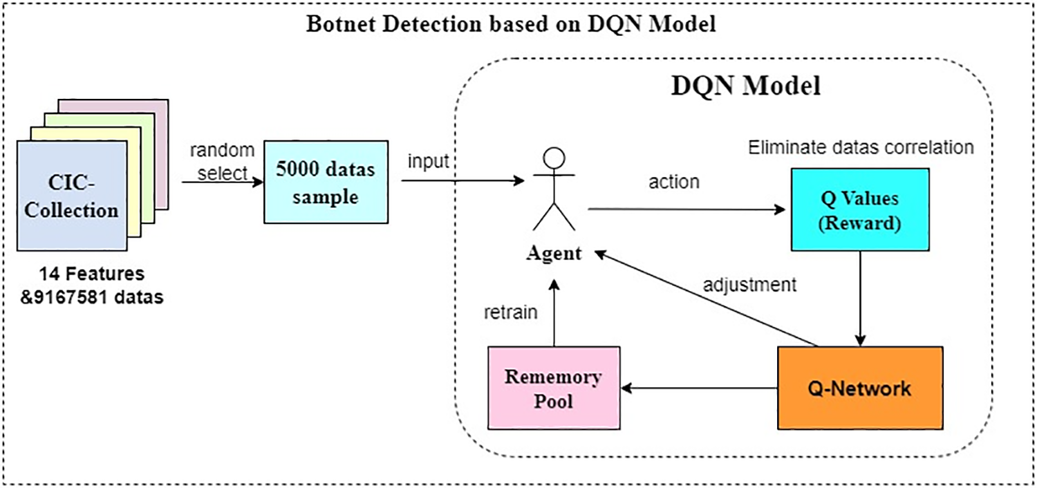
Figure 7: DQN botnet detection model

The overall pseudocode of the DQN detection model is as follows:

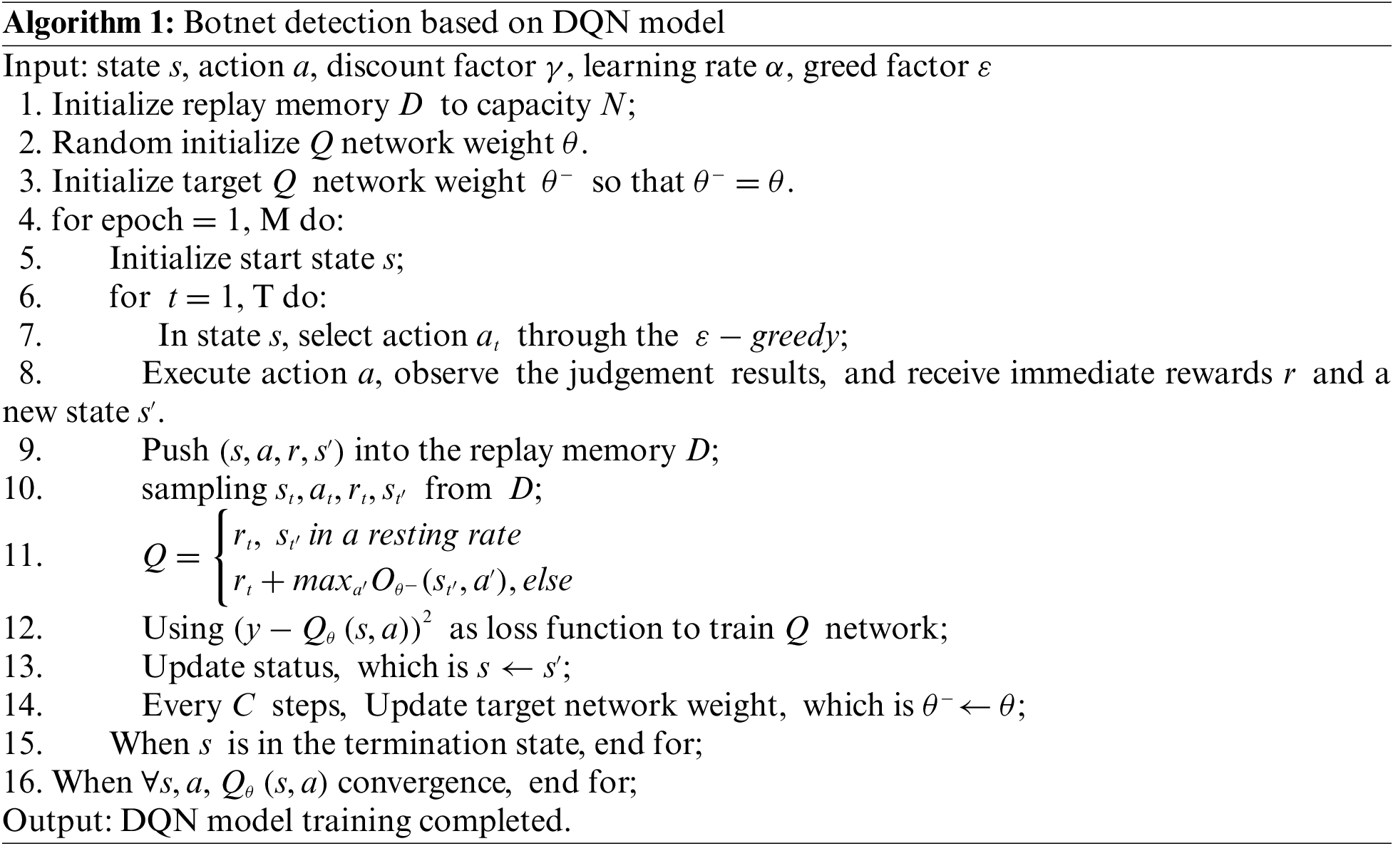
At this point, the construction of the botnet traffic detection based on the DQN algorithm is complete, and it will be used for comparison with the subsequent construction of the DDQN model.

3.3.3 DDQN Model

The DQN algorithm tends to overestimate Q-values, resulting in the detection or performance ability needing to be better in the test set than in the training set, despite having high Q-values. By examining the algorithms of Q-learning and DQN, it can be observed that the max operation is used in Eqs. (3)–(5), which idealizes the selection and evaluation of an action value. However, if function approximation and noise are present, this operation will consistently yield overestimated results. To address this issue, the DDQN algorithm decouples the two Q-value functions, updating them randomly and utilizing each other’s experiences to update the network weights θ and θ−. By separating the action selection and action evaluation, DDQN aims to avoid the problem of overestimation. The formula is shown as Eq. (7).

Q(s,a;θ−)=Rt+1+γQ[st+1,arg maxa⁡Q(st+1,a;θt);θt−](7)

In the equation, DDQN uses the maximum Q-value from the first DQN to select an action and then employs the second DQN to compute the selected action. This approach effectively avoids the issue of inaccurate Q-value estimation caused by noise and function approximation. DDQN still utilizes a greedy policy to learn the estimated Q-values but evaluates its policy using the second set of weight parameters, θ−. The exchange of θ and θ− is performed continuously to update the model. Compared to DQN, DDQN introduces relatively minor changes. However, it effectively reduces the impact of noise on DQN, resulting in more accurate detection capabilities for the botnet traffic monitoring model and preventing premature convergence during training.

Since the early stages of the algorithm are consistent with DQN, this paper adopts the pseudocode of DQN for implementation. The code is as follows:

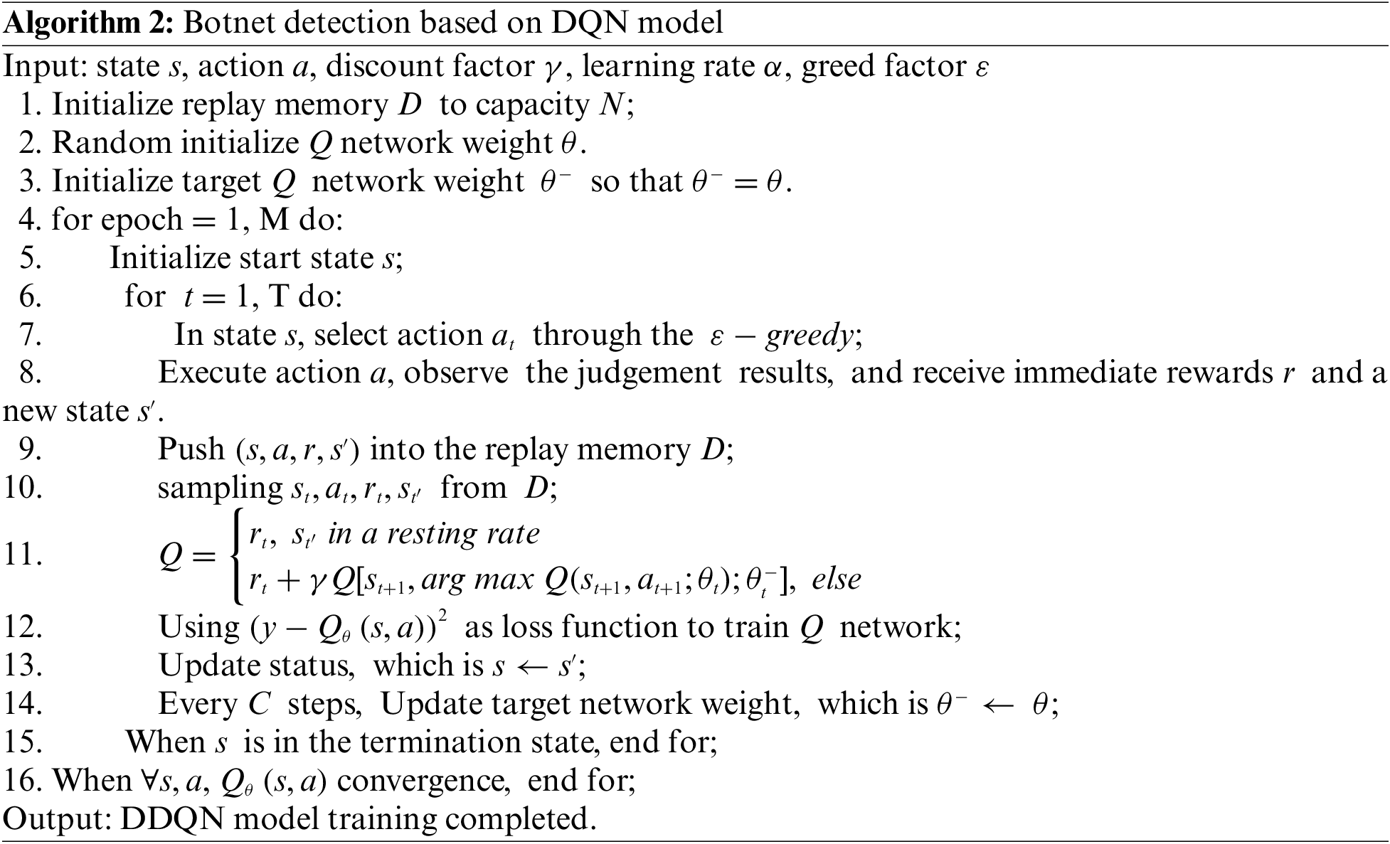
The working principle of DDQN is shown in Fig. 8.

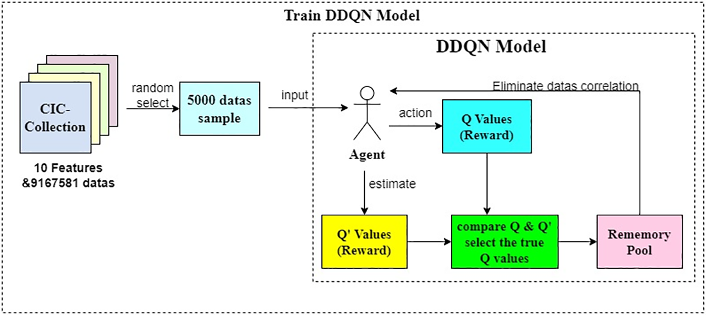
Figure 8: DDQN botnet detection model

With that, the construction of the botnet traffic detection based on the DDQN algorithm is complete.

4  Analysis of Experimental Results

4.1 Data

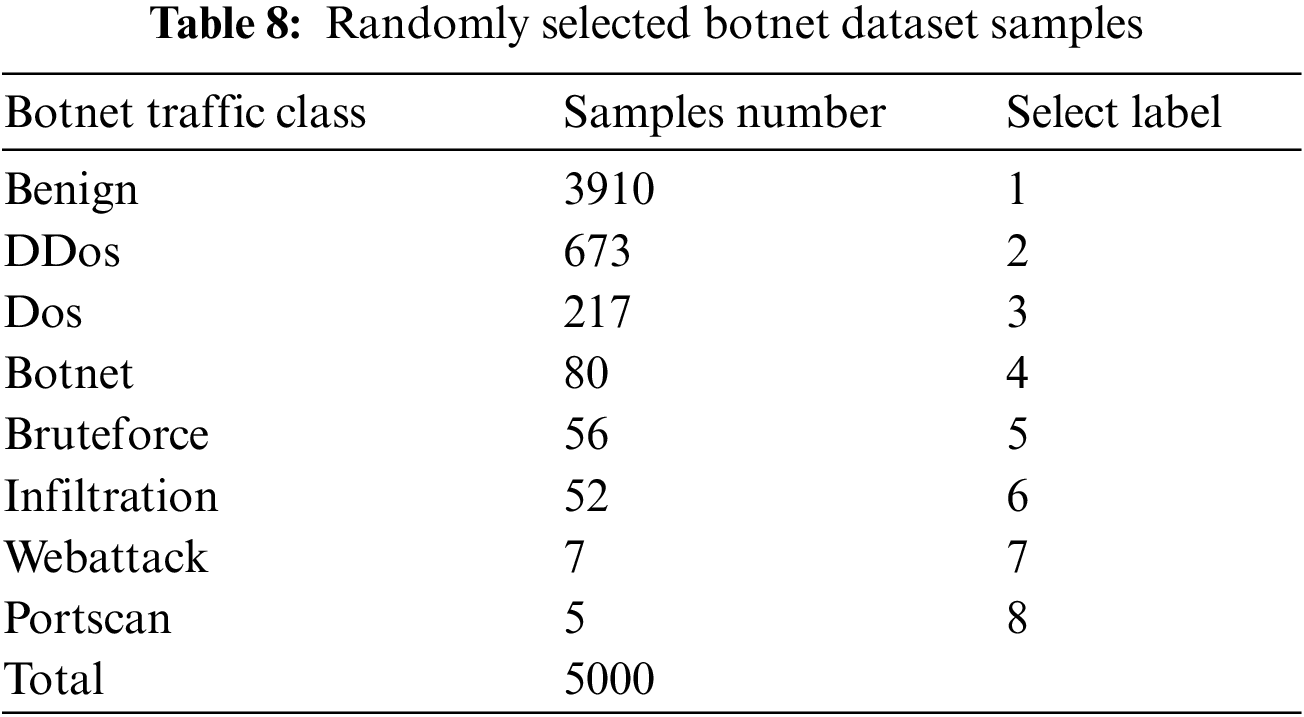
In Section 3.1, the dataset has been processed in this study. A random sample of 5000 data samples was selected according to the proportion for the experiments. The quantity and labels of the selected dataset are shown in Table 8.

4.2 Model Assessment

In this study, an additional set of 5000 samples was selected from the dataset using the same method described earlier as the test set. Two approaches were employed for feature classification: One using the OneR classifier and the other randomly selecting 10-dimensional features. These features were then separately inputted into the DQN and DDQN detection models. The Q-values of DDQN and DQN were compared, followed by the comparison of their precision and accuracy. Based on these observations, the conclusions of the experiment were drawn. The formulas for calculating accuracy and precision are as follows:

Accuracy=TP+TNTP+TN+FP+FN(8)

Precision=TPTP+FP(9)

In Eqs. (8) and (9), TP represents true positive, which refers to the positive samples correctly predicted as positive by the model. TN represents true negative, which refers to the negative samples correctly predicted as unfavorable. FP represents false positive, which refers to the negative samples incorrectly predicted as positive by the model. FN represents false negatives, which refers to the positive samples incorrectly predicted as unfavorable.

4.2.1 Model Comparison with OneR Classifiers in CIC-Collection Test Set

In this experiment, The 10 features selected by the OneR classifier, as mentioned in Section 3.2, are used for training. The comparison of Q-values between the models is shown in Fig. 9.

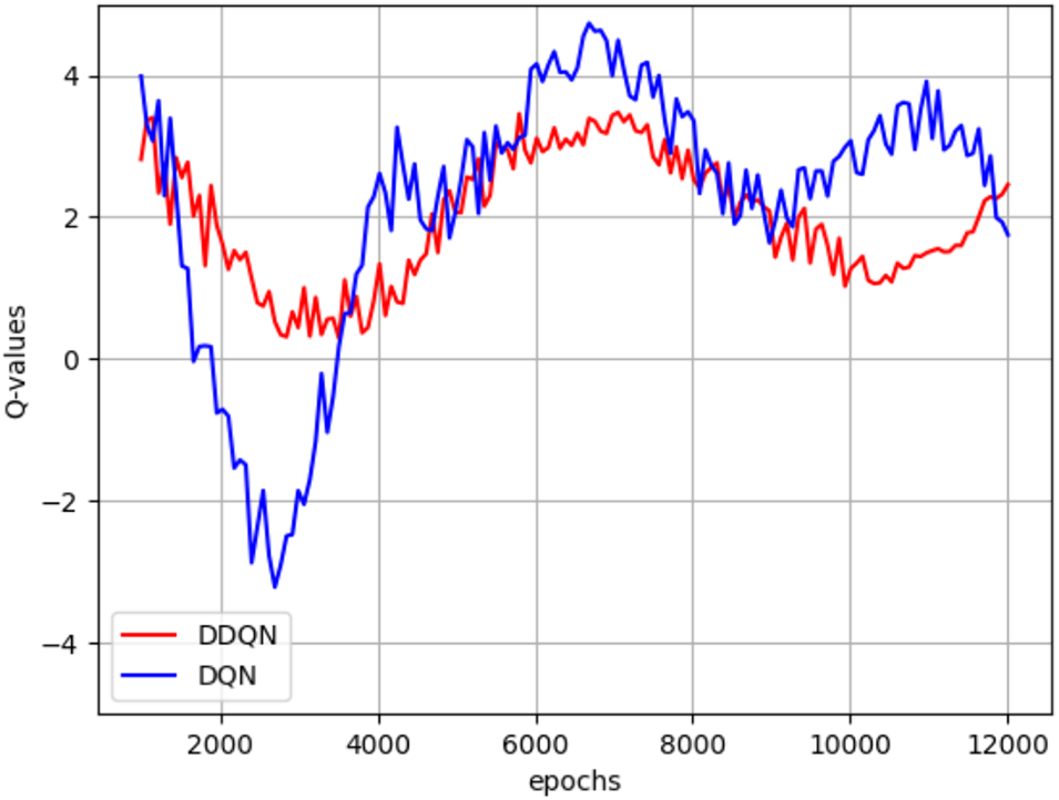
Figure 9: Comparison of Q-values

It can be observed that, compared to DQN, DDQN does not frequently change its policy, resulting in less fluctuation in Q-values. Although DDQN does not achieve the same high score as DQN (4.3241), it also avoids the meager score (−3.1224). Overall, DDQN improves the stability of the model’s predictions.

Next, we introduced the LSTM detection model to compare it with the two models to observe their judgment capabilities. The comparison of the accuracy and precision of the three models is shown in Fig. 10. Since all data of the three models are higher than 0.5, the ordinate range of the line chart in Fig. 10 is set between 0.5–1.

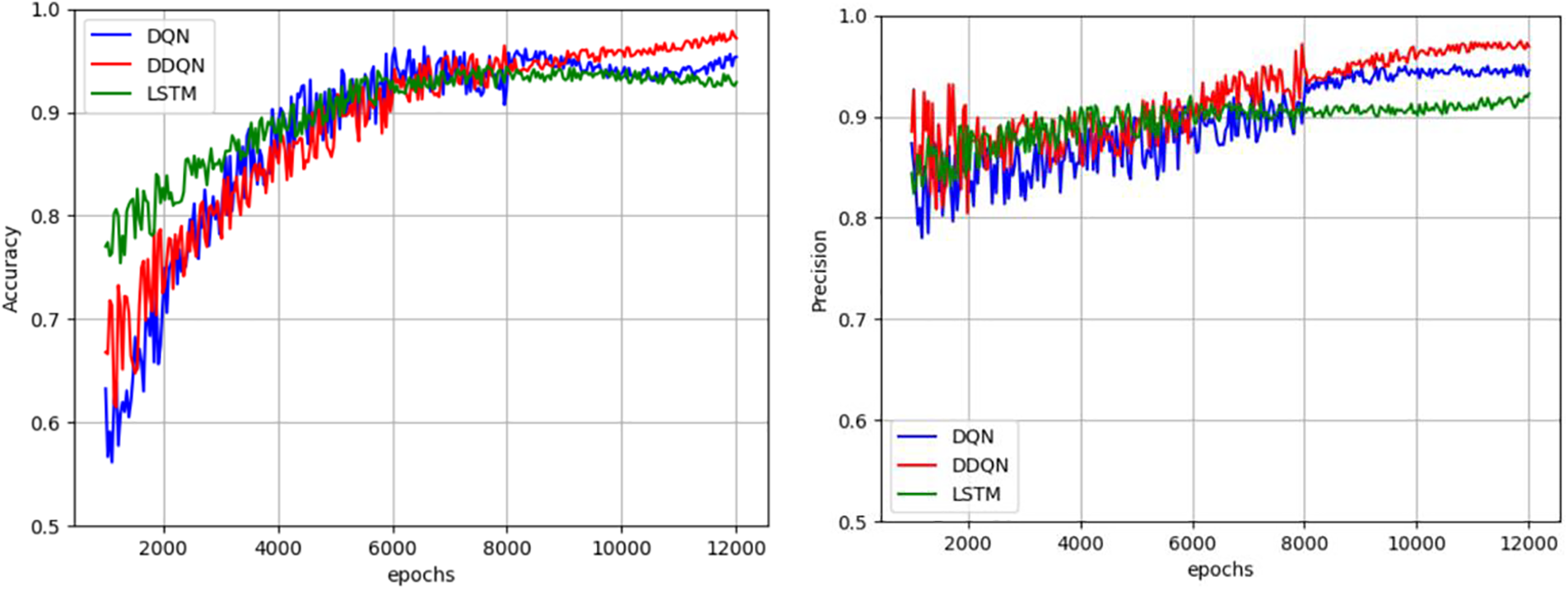
Figure 10: Comparison of accuracy and precision between DQN detection model and DDQN detection model

From the figure, it can be found that although DDQN initially had lower accuracy in processing the test set than DQN, due to its dual Q-value characteristic, the accuracy after convergence was significantly higher than DQN, and DDQN completely outperformed DQN in terms of accuracy. From these two evaluation indicators, it can be concluded that DDQN has significantly stronger stability and adaptability than DQN; The difference between the two models and LSTM is not significant, and in terms of precision, DDQN and DQN are better than LSTM detection models after convergence.

However, the use of test sets alone cannot directly reflect the advantages of the Deep reinforcement learning DDQN detection model and DQN detection model over the deep learning LSTM detection model, nor can it fully reflect the superiority of the DDQN detection model over the DQN detection model, because the test sets are ultimately narrow and limited. So in the next experiment, the CIC-ISD2017 dataset mentioned in Section 3.3.1, which has more data samples and is more complex and confusing, will be used to compare the detection results of the three models again and draw the conclusion.

4.2.2 Model Comparison with OneR Classifiers in CIC-IDS2017 Datasets

In this experiment, we directly used the features provided by the OneR classifier in Section 3.2 for training and testing, intending to verify the detection ability of the three models in unfamiliar datasets under the same batch of features. The comparison of Q-values between the models is shown in Fig. 11.

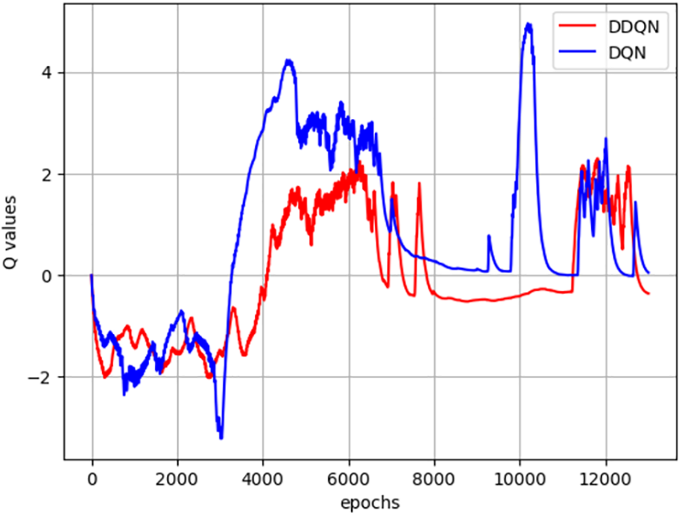
Figure 11: Comparison of Q-values between DDQN and DQN

It can be observed that despite replacing the dataset, the trend of Q-value change is consistent with the test, and it is not higher than the best case of DQN but also not lower than the worst case of DQN. DDQN still performs more stably than DQN.

Next, we introduced the LSTM detection model to compare it with the two models to observe their judgment capabilities. The comparison of the accuracy and precision of the three models is shown in Fig. 12.

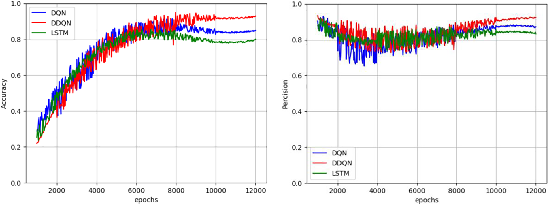
Figure 12: Comparison of accuracy and precision between DQN detection model and DDQN detection model

It can be observed that after replacing the dataset, the accuracy and precision of the three models decreased, with LSTM’s accuracy dropping to 80.42% and DQN’s dropping to 83.94%. Although DDQN decreased, it still maintained an accuracy of 90.23%; In terms of accuracy, the DDQN detection model is also better than the DQN and LSTM models. Therefore, it can be concluded that Deep reinforcement learning has a stronger adaptability than deep learning, and because DDQN has set double Q-values, its adaptability and stability have been greatly improved on the basis of the original DQN.

5  Conclusion

This paper proposes a deep reinforcement learning method based on Double DQN for botnet traffic detection models. Compared to the DQN model built in the same way, the DDQN model improves the stability of traffic detection by decoupling the selection and action, which can maintain good detection capabilities in various environments. Experimental results demonstrate that feature selection using the OneR classifier enhances the detection capability of the model. Additionally, the stability of the DDQN model enables it to adapt better to variations in different datasets. Regardless of whether feature selection is performed using the OneR classifier, the detection model constructed with DDQN outperforms the DQN detection model in terms of accuracy and precision. However, due to the parameter exchange between the target network and the leading network in DDQN, the model becomes more complex, requiring more significant time and space costs than DQN. In future research, exploring other deep reinforcement learning algorithms that can reduce time and space costs may be beneficial. Furthermore, besides the OneR classifier, other classifiers can be explored to select features and train improved botnet traffic detection models.

Acknowledgement: The authors gratefully acknowledge the anonymous reviewers for their valuable comments. It is precisely these suggestions that make this study more complete and professional.

Funding Statement: This study was supported by the Liaoning Province Applied Basic Research Program, 2023JH2/101600038.

Author Contributions: Yutao Hu was responsible for the writing of the article, and together with Xiangyu Ma, they completed the entire experimental part of the article. Yuntao Zhao checked the feasibility and standardization of the article and communicated with the journal editor as the corresponding author. Yongxin Feng approved this study and contacted and provided financial support.

Availability of Data and Materials: Not applicable.

Conflicts of Interest: The authors declare that they have no conflicts of interest to report regarding the present study.

References

1. Z. S. Zhu, G. H. Lu, Y. Chen, Z. Fu, P. Roberts and K. Han, “Botnet research survey,” in Ann. IEEE Int. Comput. Softw. Appl. Conf., Turku, Finland, 2008, pp. 967–972. [Google Scholar]

2. M. Feily, A. Shahrestani, and S. Ramadass, “A survey of botnet and botnet detection,” in Int. Conf. Emerg. Secur. Inf., Syst. Technol., Athen, Greece, 2009, pp. 268–273. [Google Scholar]

3. J. W. Qin, “Analysis of network security monitoring data for July 2022,” Internet World, vol. 7, no. 8, pp. 57–58, 2022. [Google Scholar]

4. Kaspersky Co., “In 2022, the number of human-caused cyber incidents per day increased 1.5 times,” 2023. [Google Scholar]

5. X. Y. Wang, “Analysis of the recent global cybersecurity situation and trends,” Commun. Manag. Technol., vol. 7, no. 3, pp. 53–55, 2022. [Google Scholar]

6. H. R. Zeidanloo, A. B. Manaf, P. Vahdani, F. Tabatabaei, and M. Zamani, “Botnet detection based on traffic monitoring,” in Int. Conf. Netw. Inf. Technol. (ICNIT), Manila, Philippines, 2010, pp. 97–101. [Google Scholar]

7. D. Zhao, I. Traore, and A. Ghorbani, “Botnet detection based on traffic behavior analysis and flow intervals,” Comput. Secur., vol. 4, no. 39, pp. 2–16, 2013. doi: 10.1016/j.cose.2013.04.007. [Google Scholar] [CrossRef]

8. W. Hijawi, J. Alqatawna, A. M. Al-Zoubi, M. A. Hassonah, and H. Faris, “Android botnet detection using machine learning models based on a comprehensive static analysis approach,” J. Inf. Secur. Appl., vol. 58, no. 5, pp. 1–14, 2021. doi: 10.1016/j.jisa.2020.102735. [Google Scholar] [CrossRef]

9. S. Joshi and E. Abdelfattah, “Efficiency of different machine learning algorithms on the multivariate classification of IoT botnet attacks,” in IEEE Ann. Ubiquitous Comput. Electr. Mob. Commun. Conf. (UEMCON), New York, NY, USA, 2020, pp. 0517–0521. [Google Scholar]

10. G. Kirubavathi and R. Anitha, “Structural analysis and detection of android botnets using machine learning techniques,” Int. J. Inf. Secur., vol. 2, no. 17, pp. 153–167, 2018. doi: 10.1007/s10207-017-0363-3. [Google Scholar] [CrossRef]

11. S. Anwar, J. M. Zain, Z. Inayat, A. Karim, R. Haq and A. N. Jabir, “A static approach towards mobile botnet detection,” in Int. Conf. Electr. Des. (ICED), Phuket, Thailand, 2016, pp. 563–567. [Google Scholar]

12. J. Xu, “Research on detection methods of mobile botnet,” Comput. Technol. Dev., vol. 12, no. 26, pp. 117–121, 2016. [Google Scholar]

13. A. F. Kadir, N. Stakhanova, and A. A. Ghorbani, “Android botnets: What URLs are telling us,” in Int. Conf. Netw. Syst. Secur., New York, NY, USA, 2015, pp. 78–91. [Google Scholar]

14. Z. X. Fu, Y. Xu, Z. D. Wu, D. D. Xu, and X. X. Xie, “Incremental learning based intrusion detection method for SVM KNN networks,” Comput. Eng., vol. 4, no. 46, pp. 115–122, 2020. [Google Scholar]

15. Z. Abdullah, M. M. Saudi, and N. B. Anuar, “Mobile botnet detection: Proof of concept,” in 2014 IEEE 5th Cont. Syst. Grad. Res. Colloq., Shah Alam, Malaysia, 2014, pp. 257–262. [Google Scholar]

16. D. A. Girei, M. A. Shah, and M. B. Shahid, “An enhanced botnet detection technique for mobile devices using log analysis,” in Int. Conf. Autom. Comput. (ICAC), London, UK, 2016, pp. 450–455. [Google Scholar]

17. V. Costa, S. Barbon, R. Miani, J. Rodrigues, and B. B. Zarpelao, “Mobile botnets detection based on machine learning over system calls,” Int. J. Secur. Netw., vol. 2, no. 14, pp. 103–118, 2019. doi: 10.1504/IJSN.2019.100092. [Google Scholar] [CrossRef]

18. S. Yerima and A. Bashar, “Bot-IMG: A framework for image-based detection of android botnets using machine learning,” in IEEE/ACS 18th Int. Conf. Comput. Syst. Appl. (AICCSA), Tangier, Morocco, 2021, pp. 1–7. [Google Scholar]

19. P. Torres, C. Catania, S. Garcia, and C. Garino, “An analysis of recurrent neural networks for botnet detection behavior,” in IEEE Biennial Congr. of Argentina (ARGENCON), Buenos Aires, Argentina, 2016, pp. 1–6. [Google Scholar]

20. A. Pektas and T. Acarman, “Botnet detection based on network flow summary and deep learning,” Int. J. Netw. Manag., vol. 28, no. 6, pp. 1–15, 2018. doi: 10.1002/nem.2039. [Google Scholar] [CrossRef]

21. F. Hussain et al., “A two-fold machine learning approach to prevent and detect IoT botnet attacks,” IEEE Access, vol. 23, no. 78, pp. 163412–163430, 2021. doi: 10.1109/ACCESS.2021.3131014. [Google Scholar] [CrossRef]

22. F. J. Chen, “Research on botnet detection technology based on deep learning,” Guangdong Univ. Technol., vol. 2022, no. 1, pp. 1–54, 2022. [Google Scholar]

23. Z. J. Qi, “Research on traffic detection technology for malicious networks based on neural networks,” Guangdong Univ. Technol., vol. 2022, no. 3, pp. 1–49, 2022. [Google Scholar]

24. F. Q. Lu, “Research on botnet detection technology based on deep learning,” Nanjing Univ. Post. Telecommun., vol. 2021, no. 1, pp. 1–70, 2021. [Google Scholar]

25. H. T. Xue and C. Wang, “Research on botnet traffic detection based on GAN,” Electr. Des. Eng., vol. 17, no. 30, pp. 146–149, 2022. [Google Scholar]

26. M. Volodymyr et al., “Human-level control through deep reinforcement learning,” Nature, vol. 518, no. 73, pp. 529–533, 2015. [Google Scholar]

27. H. V. Hasselt, A. Guez, and D. Silver, “Deep reinforcement learning with double Q-learning,” in Proc. Thirtieth AAAI Conf. Artif. Intell., Phoenix, Arizona, USA, 2016, pp. 2094–2100. [Google Scholar]

28. G. Zuo, T. T. Du, and J. H. Lu, “Double DQN method for object detection,” in ACM Cloud Auton. Comput. Conf., Tucson, Arizona, USA, 2017, pp. 6727–6732. [Google Scholar]

29. W. L. Wen, “Research on malicious code generation countermeasures based on deep reinforcement learning,” Guangdong Univ. Technol., vol. 2022, no. 4, pp. 1–48, 2022. [Google Scholar]

30. C. D. McDermott, F. Majdani, and A. V. Petroviski, “Botnet detection in the internet of things using deep learning approaches,” in IEEE Int. Joint Conf. Neural Netw. (IJCNN), Rio de Janeiro, Brazil, 2018, pp. 8–13. [Google Scholar]

31. A. Venturi, G. Apruzzese, M. Andreolini, M. Colajanni, and M. Marchetti, “DReLAB—deep reinforcement learning adversarial botnet: A benchmark dataset for adversarial attacks against botnet intrusion detection systems,” Data in Brief, vol. 33, no. 1, pp. 1–12, 2020. [Google Scholar]

32. D. Wu, B. X. Fang, J. N. Wang, Q. X. Liu, and X. Cui, “Evading machine learning botnet detection models via deep reinforcement learning,” in IEEE Int. Conf. Commun. (ICC), Shanghai, China, 2019, pp. 192–198. [Google Scholar]

33. G. Apruzzese, M. Andreolini, M. Marchetti, A. Venturi, and M. Colajanni, “Deep reinforcement adversarial learning against botnet evasion attacks,” IEEE Trans. Netw. Serv. Manag., vol. 4, no. 17, pp. 18208–18212, 2020. doi: 10.1109/TNSM.2020.3031843. [Google Scholar] [CrossRef]

34. R. H. Randhawa, N. Aslam, M. Alauthman, M. Khalid, and H. Rafiq, “Deep reinforcement learning based evasion generative adversarial network for botnet detection,” arXiv preprint arXiv:2210.02840, 2021. [Google Scholar]

35. R. Brereton, “One-class classifiers,” J. Chemometr., vol. 17, no. 25, pp. 225–246, 2011. [Google Scholar]