Pervasive Attentive Neural Network for Intelligent Image Classification Based on N-CDE’s

1  Introduction

Image recognition encompasses several techniques for automatically assigning one or many labels to an image, depending on its visual contents. This task, which can be categorized into multi and single labelled image class, is both underlying and applicable in practice. Convolutional Neural Networks (CNNs) have also achieved tremendous success in recent times [1–3]. Recently, researchers have employed the CNNs in human action recognition [4,5], document classification [6], blockchain security [7] and superhero classification [8]. Nevertheless, the efficacy of CNNs remains relatively constrained when confronted with demanding image recognition tasks. Illustrated in Figs. 1a and 1b are representative images and their respective class, extracted from the MS COCO [9] and PASCAL VOC dataset [10], serving as instances of Fine-Grained Visual Categorization (FGVC) and image classification.

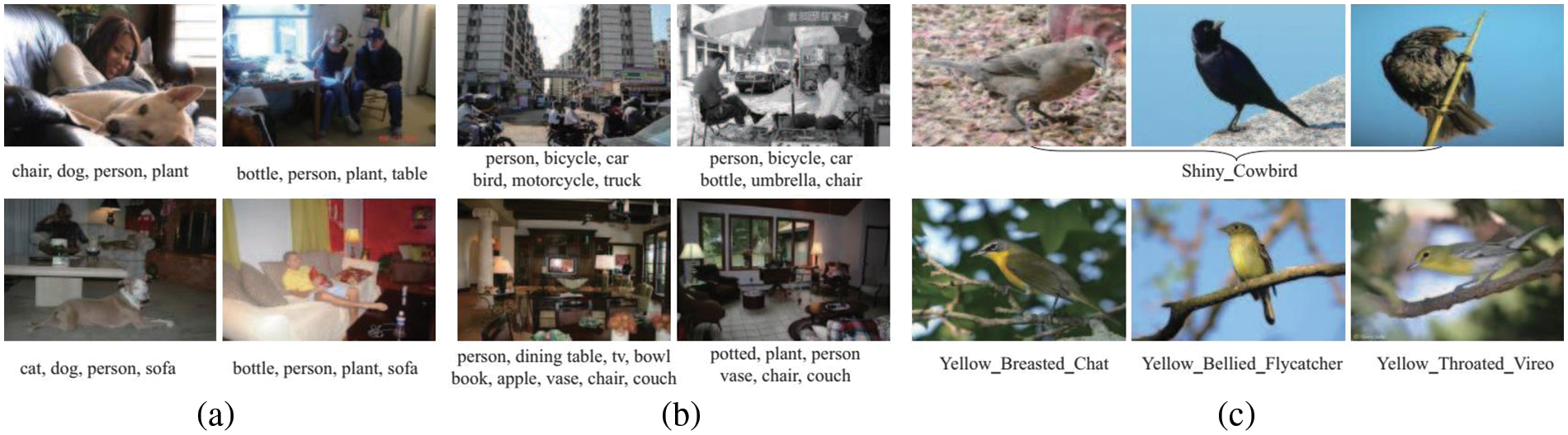
Figure 1: A selection of representative images obtained from various datasets [9–11]

A form of differential equation that includes a control input or a decision-making mechanism is referred to as a Controlled Differential Equation (CDE). These equations delineate the temporal evolution of a system’s state within the framework of dynamic systems and control theory. They account for both the inherent dynamics of the system and the impact of external controls. To define the specific terminology: a) Differential Equation (DE): DEs of functions are utilized in this type of equation. These derivatives represent the rates of change of particular variables in the context of CDE’s; and b) Controlled: The term “controlled” denotes the circumstance in which a control input influences or directs the behavior of the system. The control input in question is commonly a programmable function that can be altered or tailored to accomplish intended system operations. Consequently, a CDE delineates the temporal evolution of a system's state, incorporating not only the intrinsic dynamics of the system but also the influence of a control input. In mathematical notation, a CDE may be represented as dxdt=f(x,u), here, x denotes the system’s state variables, t signifies time, u signifies the control input, and f represents a function describing the system’s natural evolution.

The presence of several factors such as viewpoint, occlusion, illumination, scale and appearance contribute to the substantial intra-class variations observed in picture identification. These factors, along with the interplay between different object categories, provide considerable challenges and render image classification a more complex task. Additionally, Fig. 1c depicts a collection of bird photos and their respective class sourced from CUB-200-2011 dataset [11], which is recognized as a demanding dataset comprising 200 distinct bird species. The presence of significant intraclass variances resulting from factors such as pose, scales, and position, along with the small changes between classes, contribute to the challenging nature of FGVC. One may pose the question: Is it possible to develop a methodology that possesses the capacity to augment the efficacy of representation?

It is most likely possible to relate the observed performance disparities between N-CDE’s and Neural Ordinary Differential Equations (NODE’s) to certain architectural variations and innate traits that are ingrained in the models. Different architectural features such as attention processes, network depth, skip connections, and complexity may be responsible for different information-capturing and information-using capacities. The phenomenon of image analysis has been the subject of substantial research in previous studies since it has been recognized as an efficient method for enhancing the representation capabilities of machine learning in multiple domains like object recognition [12–14], image denoising [15], detection of human movement [16], CPU scheduling [17], target detection [18], person identification [19] and Spoof detection [20]. Furthermore, intrinsic features like data augmentation, learning rate tactics, regularization approaches, and parameter initialization can have a significant impact on how well the models generalize and learn. The details in how these components are implemented within the architectures, in addition to taking the difficulty of the task and the structure of the dataset into account, are important factors affecting the observed differences in model performance. Referring to the original research papers or documentation related to N-CDE’s, and NODE’s is crucial for a thorough understanding because these sources usually offer in-depth explanations of the experimental conditions, hyperparameter settings, and architectural decisions that lead to the differences that are observed [21].

When compared to N-CDE’s, the use of NODE’s in attention-based models may have certain drawbacks. Due to the complexity of attention systems, one significant obstacle is the possible difficulty in comprehending the decisions made by the model. Comprehending the logic behind the model’s concentration on input data areas could be intricate, impeding the model's clarity and comprehensibility. Furthermore, the scalability of the model may be impacted by the computational complexity brought about by attention processes, particularly if they are widespread or complicated and result in longer training durations and higher resource requirements. Attention-based models have a danger of overfitting, especially if they do not have good regularization techniques, and they might not translate well to new, untested data. Potential drawbacks include these models’ sensitivity to hyperparameter decisions as well as their reliance on the variety and distribution of the training set. Standardization issues in attention mechanisms, such as NODE’s, might make it difficult to compare them across various architectures, and their efficacy in tasks requiring a more comprehensive contextual awareness may be restricted by their inability to capture long-range dependencies. Furthermore, the resilience of attention-based models in practical applications may be questioned due to their susceptibility to adversarial attacks. It is crucial to remember that the specific shortcomings of NODE’s and how they compare to N-CDE’s will vary depending on how well each architecture is implemented [22].

An advanced method to improve neural network modeling is the combination of N-CDE and attentive neural networks to generate attentive N-CDE’s. The underlying idea is to combine N-CDE’s—which are well-known for their capacity to simulate dynamics in continuous time—with attention mechanisms that allow for the selective focus on important aspects. This combination enables the dynamic adaptation to important features at different time points and enables the modeling of temporal dynamics using differential equations in attentive N-CDE’s. This is particularly useful for time-series data, where it is essential to capture changing patterns over time. Moreover, the inclusion of attention mechanisms makes it easier to create attention maps, which offers insight into the temporal events that affect the model’s predictions. The promise of this combined method in managing complex and dynamic data structures is demonstrated by the synergy between N-CDE’s and attention processes, which not only increases interpretability in time-series analysis but also strengthens the model’s robustness to noisy or irregular temporal patterns [23].

Over the course of time, persistent initiatives have been undertaken to tackle the concerns. A new methodology of arranging feature information with a class specific weight along with an extra approach to improve the impact of the feature information arrangement was introduced to comprehensively handle classification and localization misalignment. The results showed MaxBoxAccV2 score of 68.9% and 79.5% on CUB-200-2011 and ImageNet-1K datasets, respectively. A clustering-based approach that is Class RE-Activation Mapping (CREAM) was applied on class specific background context-embeddings as cluster centers and contextual embeddings were learned during training by CAM-guided momentum preservation approach. CREAM performed well on OpenImages, ILSVRC and CUB benchmark datasets [9]. A pipeline for DA-WSOL was devised with the aim of incorporating domain adaption (DA) methodologies into WSOL by utilizing target sampling strategy to choose various sorts of target samples and experiments showed better results from SOTA methods on multi benchmark.

Class-agnostic Activation Map (CAM), a contrastive learning approach, utilized unlabeled images data without relying on image-level supervision and reported to successfully extract object bounding boxes [24]. CNN in conjunction with Recurrent Neural Network (RNN) was utilized for defining image-label relationship and the semantic label dependence. The experimental results of RNN-CNN outperformed multi-label classification models [25]. The regional latent dependencies model was developed which comprises a full convolutional localization model to locate the region and the located regions are then forwarded to the RNN for characterization of dependences at the regional level. They claimed the best performance of model for predicting small objects [26].

The evaluation of the depth of the convolutional network was conducted using an architecture that employed compact (3 × 3) convolution filter, which revealed that by increasing the depth to 16–19 weight layers, a notable enhancement in performance was attained compared to previous configurations [27]. A framework for residual learning was developed, which obtained good generalization performance on recognition tasks by explicitly reformulated layers as learning residual parameters in relation to corresponding layers, as opposed to learning unreferenced functions [28]. Multi labelled image recognition was achieved by proposing a recurrent memorized attention-based module, consisting of an LSTM and transformer layer subnetwork. They reported better results for both accuracy and efficiency on PASCAL VOC 07 and MS COCO dataset [29].

Multi object recognition was performed by extracting object proposals using selective search, which yielded two distinct types of extracted features. The LMNN CNN was provided with a low-dimensional feature to generate the label view, while the normal CNN feature was employed as the feature view and then these two views were fused. The results validated discriminative effect and the generalization capability of the model [30]. A novel attention framework utilizing reinforcement learning was devised to address the problem of redundant computation cost by iteratively identifying a series of attentional and informative regions associated with semantic objects. On MS COCO and PASCAL VOC, this technique outperformed in efficiency and region-specific picture labelling [31].

Reinforcement learning approach to classify multi class images that seeks to replicate human behavior in order to assign labels to images from simple to complex was utilized to sequentially predict labels [32]. RNN model with an attention layer as well as LSTM layer was used for multi labelled image recognition to jointly learns the labels of interest and results proved to be effective on MS COCO and NUS-WISE datasets [33]. A unique deep learning architecture was constructed that integrates knowledge graphs to represent the connections among multiple labels and learns information from semantic label bay. The proposed methodology exhibited enhanced performance in the context of multi labelled recognition and multi labelled zero-shot learning (ML-ZSL) [34].

Attention maps were generated from Spatial Regularization Network (SRN) and results obtained from regularized network were merged with original outcomes by a ResNet-101 model, and SRN model demonstrated improved classification performance for both spatial and semantic relationships of labels [35]. An effective attention module called Convolutional Block Attention Module (CBAM) was developed with the ability to integrate with CNN architecture, resulting in minimal computational overhead [36]. A novel model called Squeeze-and-Excitation (SE) was designed which dynamically adjusts channel wise feature retorts by overtly capturing the mutuality among channels. The SENet architecture was constructed by concatenating many SE blocks, resulting in a significant reduction in top-5 errors to a value of 2.251% [37].

Although N-CDE’s exhibit potential in representing dynamic dependencies in neural network models, significant research gaps still need to be filled. First, more research is needed to determine how well N-CDE’s scale and perform when handling huge datasets or intricate model architectures. Real-world applications require an understanding of the computational demands and potential obstacles. Furthermore, studies might explore N-CDE interpretability in further detail, focusing on how reliable and understandable these models are, particularly when used for challenging tasks. Moreover, evaluating N-CDE’s adaptation to different real-world settings requires examining their generalization abilities over a range of datasets and domains. Another area that needs attention is the creation of strong training procedures, regularization approaches, and methodologies for dealing with problems like overfitting or underfitting. Finally, comparisons with other dynamic modeling techniques can shed light on the advantages and disadvantages of N-CDE’s, leading to a more thorough comprehension of their suitability in various situations. Filling in these research voids will help N-CDE’s mature and become more widely used in dynamic modeling applications.

2  Attentive N-CDE’s

In NODE’s, a time series multivariate vector w(t1) at any time (t1) which can be computed by initial vector w(t0) by w(t1)=w(t0)+∫tot1g(w(t);∅g)dt, where the value of time point tj∈[0,𝒯]. Here it is noted that g is neural network having a parameter ∅g and a time dependent derivative term w. So, it can be said that the fundamental evolutionary technique information of w after being initialized lies in g. A lot of models include w but they have no limitations to heat-diffusion process, climate, and epidemic model. Though, the model which directly calculate w like RNN’s are known as discrete while the NODE’s models are continuous with respect to time t. In the integral term the time variable is controlled freely, e.g., t1 as shown above with the help of which at any time t,w can be found.

As compared with NODE’s, the starting process assumptions are more complicated than N-CDE’s, the integral used in it is known as Riemann-Stieltjes, i.e., w(t1)=w(t0)+∫tot1g(w(t);∅g)dV(t). If the identity function with respect to variable t, i.e., V(t)=t is used then N-CDE’s are reduced to NODE’s. As the controlled parameter of NODE’s is “t” and N-CDE’s have a time series V(t). Therefore, N-CDE’s could also be taken as NODE’s generalization.

Another important feature is that the multiplication of matrix vector g(w(t);∅g) dV(t) is done without requiring huge computational cost. Fig. 2 shows the general architecture of N-CDE’s, whereas in Fig. 3, it is shown that N-CDE’s of two types are used in proposed Attentive N-CDE’s technique with one N-CDE’s attention values are generated and the other one is used for initialization of w(). Two distinct attention techniques are used in proposed scheme one is known as “Time-wise attention”, called Bottom N-CDE’s in which attention value is given as 0≤α(t)≤1 and the other one is known as “Element-wise attention”, called Top N-CDE’s whose attention value α(t)∈[0,1]dim⁡V(t). The direction V and attentions of bottom N-CDE’s are concatenated, which is represented by ⊗ symbol. In these two cases, initialize second N-CDE’s by V(t) and attention element wise multiplication represented by Z(t), in this way, the input values of N-CDE’s are selected by the first N-CDE’s variable V(t). A training technique is proposed that ensures the training problem is adequately posed.

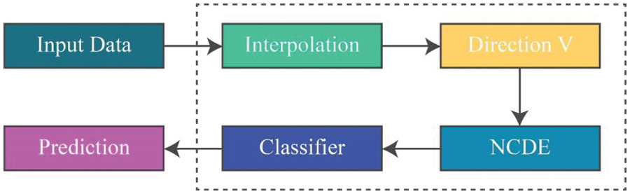
Figure 2: General architecture of N-CDE’s

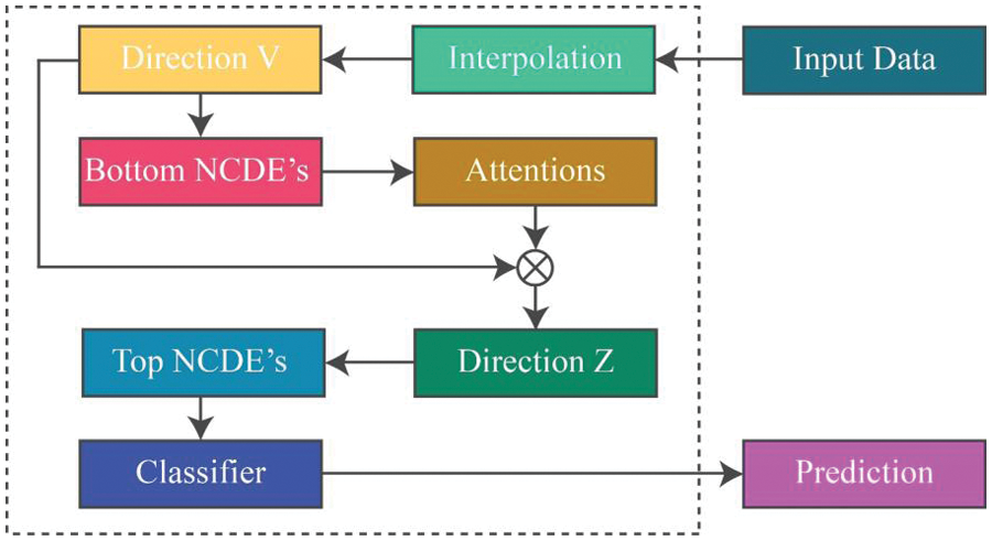
Figure 3: General architecture of proposed attentive N-CDE’s

2.1 Neural ODE’s

NODE’s are used to provide the solutions of Initial Value Problems (IVP) that contain integral terms for the calculation of w(t1) via w(t0):

w(t1)=w(t0)+∫tot1g(w(t);∅g)dt,(1)

where, the ODE’s (Ordinary Differential Equations) g(w(t);∅g) is neural network used for the approximation of w ′(t)(i.e.,w ′(t)=dwdt). For the solution of integral term NODE’s commonly used solvers for ODE’s that mainly includes Euler Method, Modified Euler, Runge Kutta Methods (RK-Method), and Dormand-Prince (RKDP) method for higher order ODE’s. Fig. 4 depicts NODE’s conventional architecture.

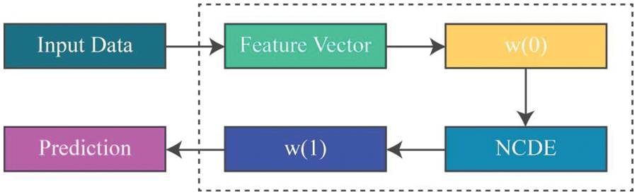
Figure 4: General architecture of NODE’s

Generally, to discretize the time variable (t) and conversion of integral into other additional step ODE’s solvers are utilized. For example, explicit Euler’s technique in one step is written as follows:

w(t+h)=w(t)+hg(w(t);∅g),(2)

where, h represents the Euler’s method step size. The RKDP technique utilize more advanced technique for updating w(t+h) from w(t) and it helps to control step size (h) dynamically. But sometimes the ODE’s solvers may cause numerical instability. For example, RKDP technique occasionally results in underflow error because it reduces the step size. Several other techniques were also suggested for the prevention of these unexpected issues. The adjoint sensitivity approach, which is employed for its effectiveness and theoretical accuracy, is utilized to develop NODE's in the context of backpropagation technique.

Consider the optimizing scalar valued loss-function ℒ(), the input of this function is derived from results of ODE’s solver.

ℒ(𝔀(t1))=ℒ(𝔀(t0)+∫tot1g(w(t);∅g)dt=ℒ(ODESolve(w,t0,t1,g,∅g));(3)

For the optimization of ℒ, gradient with respect to ∅g is required. Let us consider the adjoint quantity αw(t)=∂ℒ∂w(t), for loss function ℒ, the calculation of gradient for loss with respect to (w.r.t) parameters with the help of integral reverse mode is given as:

grad∅g(ℒ)=−∫t𝓷t0αw(t)𝒯∂g(w(t);∅g)∂∅gdt,(4)

gradw(0)ℒ and the gradients can be propagated backwards to parts before ODE’s. It is important to note that time complexity of adjoint sensitivity is 𝒪(1), while trained NODE’s complexity is proportional to quantity of RKDP steps. Both the techniques have similar time-complexities, but the efficiency of adjoint-sensitivity is quite better than backpropagation techniques. So, it helps to train NODE’s more efficiently.

2.2 Neural CDEs

One drawback observed in NODE’s is that, if given ∅g, w(t1) is determined solely based on w(t0), which raises concern regarding the capability of NODE’s for representation learning. To address this limitation, N-CDE’s used given time-series data to introduce a supplementary path denoted as V(t). Consequently, the formulation for w(t1) is now regulated by both w(t0) and V(t).

The formulation of the Initial Value Problems (IVP’s) for N-CDE’s are expressed as follows:

w(t1)=w(t0)+∫tot1g(w(t);∅g)d(V(t))(5)

w(t1)=w(t0)+∫tot1g(w(t);∅g)dV(t)dtdt,(6)

where, V(t) characterizes a natural cubic-spline path, originating from the inherent time series data. It is noteworthy that this integral problem is quoted as the Riemann-Stieltjes integral, a departure from the traditional Riemann integral employed by NODE’s. Furthermore, CDE’s function g(w(t);∅g) is introduced to approximate dw(t)d(V(t)). While various methods can be employed for determining V(t), the authors prefer natural cubic spline method because of its advantageous characteristics such as being twice differentiable, computationally efficient, and ensuring the continuity of V(t) concerning t after interpolation.

2.3 Overall Workflow

Initially, a continuous path V(t) utilizing standard cubic-spline technique is constructed by assumed data of time series, i.e., (v0,t0),(v1,t1),…. Initialize N-CDE’s from bottom by V(t) for production of attention outputs at every point of time t. Attention element wise multiplication and function V(t) used in creation of the path values Z(t) in Eq. (15). Now, initialize the N-CDE’s from top for the generation of hidden last vector. Eq. (19), contains additional classified layers which generate outcome. Besides of, raw points {(v0,t0),(v1,t1),…,(vm,tm)}, irregular and discrete behavior of given data V(t) path shows continuous behavior also V(tm)=vm, where the time tm is calculated by vm. All other non-calculated points were interpolated by cubic-spline technique using nearest data set. Fig. 5 shows the overall design of the anticipated prototype.

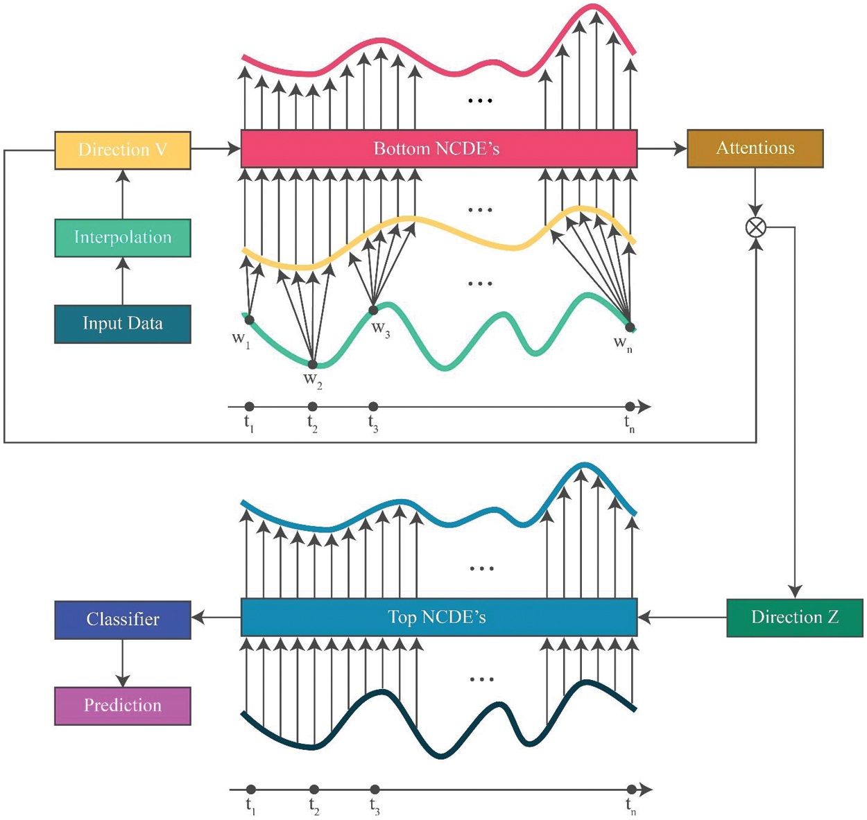
Figure 5: Overall design of the anticipated attentive N-CDE’s

2.4 N-CDE’s Vs NODE’s

Initially, a continuous path V(t) utilizing standard cubic-spline technique is constructed by assumed data of time series, i.e., {(v0,t0),(v1,t1),…}. Initialize N-CDE’s from bottom by V(t) for production of attention outputs at every point of time t. Attention element wise multiplication and function V(t) used in creation of the path values Z(t) in Eq. (15). Now, initialize the N-CDE’s from top for the generation of hidden last vector. Eq. (19) contains additional classified layers which generate outcome. Besides of, raw points {(v0,t0),(v1,t1),…(vm,tm)}, irregular and discrete behavior of given data V(t) path shows continuous behavior also V(tm)=vm, where the time tm is calculated by vm. All other non-calculated points were interpolated by cubic-spline technique using nearest data set.

The existence of path V(t) is main key point that distinguish between N-CDE’s and NODE’s techniques. In N-CDE’s, V(t) is calculated particularly by cubic spline which utilized upcoming data values {vt ′},t ′>t, in combination with its recent and previous calculations, which is the limitation in NODE’s. Hence, N-CDE’s is comparatively better than NODE’s technique. Also, N-CDE’s are converted to NODE’s by V(t)=t which is commonly known as identity function.

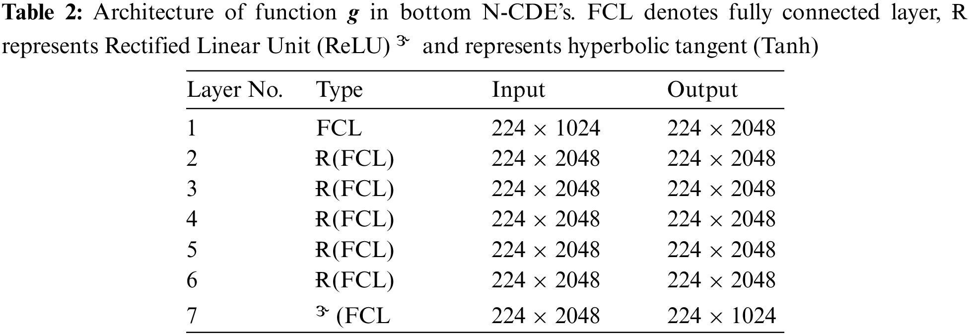
2.4.1 Bottom N-CDE’s for Attention Values

The bottom N-CDE’s is formulated as follows:

s(t1)=s(t0)+∫tot1g(s(t);∅g)dV(t);(7)

=s(t0)+∫tot1g(s(t);∅g)dV(t)dtdt(8)

Here,s(t) represents attention hidden vector and used for its derivation at time t. Here our article will support two attention concepts, i.e., attentions depending on time α(t)∈R and element α(t)∈Rdim⁡(V(t)). In the first type, the output size is 1 for a fully connected layer ℱ𝒞1, here α(t)=sigma(ℱ𝒞1(s(t)), represents scalar value. However, the roles are reversed in second type, where α(t)=sigma(s(t)) is a vector. Our observation indicates equivalence between bottom N-CDE’s and the original N-CDE’s setting.

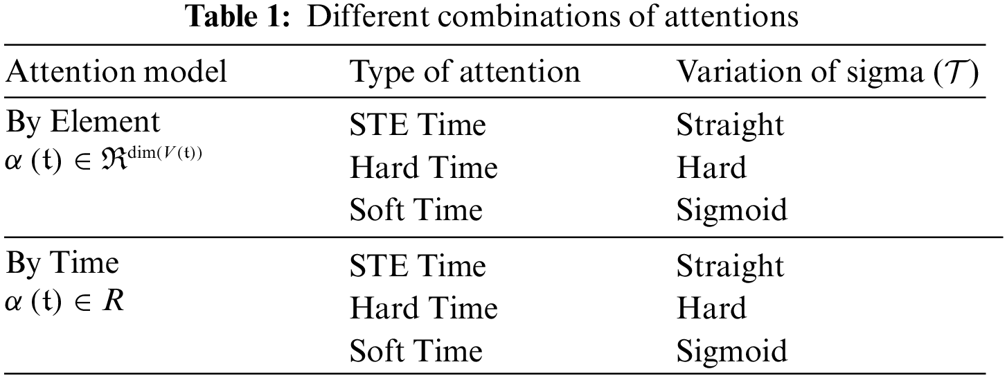
These attention types are associated with different output sizes and activation functions. In our study, we will study three variations of the sigmoid activation function. The first two are soft attention and hard attention utilizing the original sigmoid represented. Hard attention would later be finished with rounding function. The third variation will be hard attention with sigmoid slope annealing referred to as straight through estimator. We will disregard soft attention on the count of using original sigmoid. The forward and backward paths definitions for hard attention are given as:

For forward-path,

sigma(v)=ceil(sigmoid(v));(9)

For backward path,

grad(sigma(v))=grad(sigmoid(v));(10)

In straight through estimator, for forward-path,

sigma(v)=ceil(sigmoid(𝓣𝓿));(11)

For backward path,

grad(sigma(v))=grad(sigmoid((𝓣𝓿));(12)

Notably, the temperature parameter 𝒯 controls the slope of the sigmoid function.

Slope of sigmoid function is controlled via temperature 𝒯 such that 𝒯 ≥ 1.0 is a scalar. For a significantly large 𝒯, slope of the sigmoid function approaches that of the rounding function. Hence, after initializing it to 1 at the start, we uniformly keep increase 0.12 to 𝒯 every epoch. In soft time attention, the distribution is combined with the features of the localized portion, in hard time, attention uses stochastic models like the Monte Carlo Method and reinforcement learning, making it less popular, while in Space, Time, and Environment (STE), all factors of soft and hard are integrated. Table 1 shows all six, possible attention models that we retained by using three types of attention (soft time, hard time and STE time) and three variations for sigma.

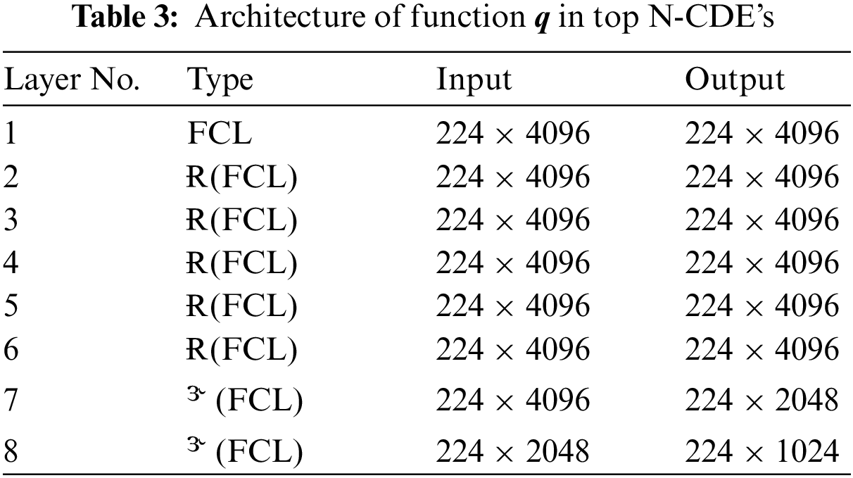
2.4.2 Top N-CDE’s for Classification

The top N-CDE’s is expressed as follows:

w(t1)=w(t0)+∫tot1q(w(t);∅q)d(Z(t));(13)

=w(t0)+∫tot1q(w(t);∅q)dZ(t)dtdt(14)

Z(t)={α(t)V(t)ifattentionistimewiseα(t)⊗V(t)ifattentioniselementwise(15)

Given here, Z(t) is the element wise multiplication between attention and V(t).⊗ represents the element-wise multiplication operation. Being able to store information picked by the bottom N-CDE’s in Z(t), top N-CDE’s is free to only concern itself with useful information and consequently downstream Machine Learning (ML) tasks can be. Therefore, Z(t) includes information chosen by the bottom N-CDE’s. The top N-CDE’s can exclusively emphasis on valuable data, leading to an enhancement in the performance of subsequent ML tasks.

Further derivation of the above equation in tractable form as:

w(t1)=w(t0)+∫tot1q(w(t);∅q)dZ(t)dtdt(16)

For attention in time wise,

dZ(t)dtdt=dV(t)dtα(t)+V(t)α(t)(1−α(t))(dℱ𝒞1(s(t))ds(t))(ds(t)dt)(17)

For attention in element wise,

dZ(t)dtdt=dV(t)dtdtα(t)+V(t)α(t)(1−α(t))(ds(t)dt)(18)

We highlight that our derivations primarily assume soft attention but remain applicable to hard-attention and straight through estimator. These attention mechanisms facilitate the selection of relevant values by the top N-CDE’s, enhancing the execution of downstream ML tasks. The generated value by hard attention lies in set {0,1} and the interval values in [0,1] are caused by soft attention. The architectures of function g in bottom N-CDE’s and q in top N-CDE’s are given in Tables 2 and 3, respectively.

Hence, it is noted that the hard-attention range is still valid. For example, consider that if attention is calculated time wise and by hard attention the value of α(t) is either 0 or 1. Consequently, dZ(t)dt=0 or dZ(t)dt=dV(t)dt that correspond exactly to proposed attention motivation, which have the concept that the top values of N-CDE’s are chosen by the bottom values N-CDE’s. Estimator of straight through is taken as a hard-attention variant of temperature annealing, which also produced values that are either 0 or 1. So the equations are easily used in all three defined attentions.

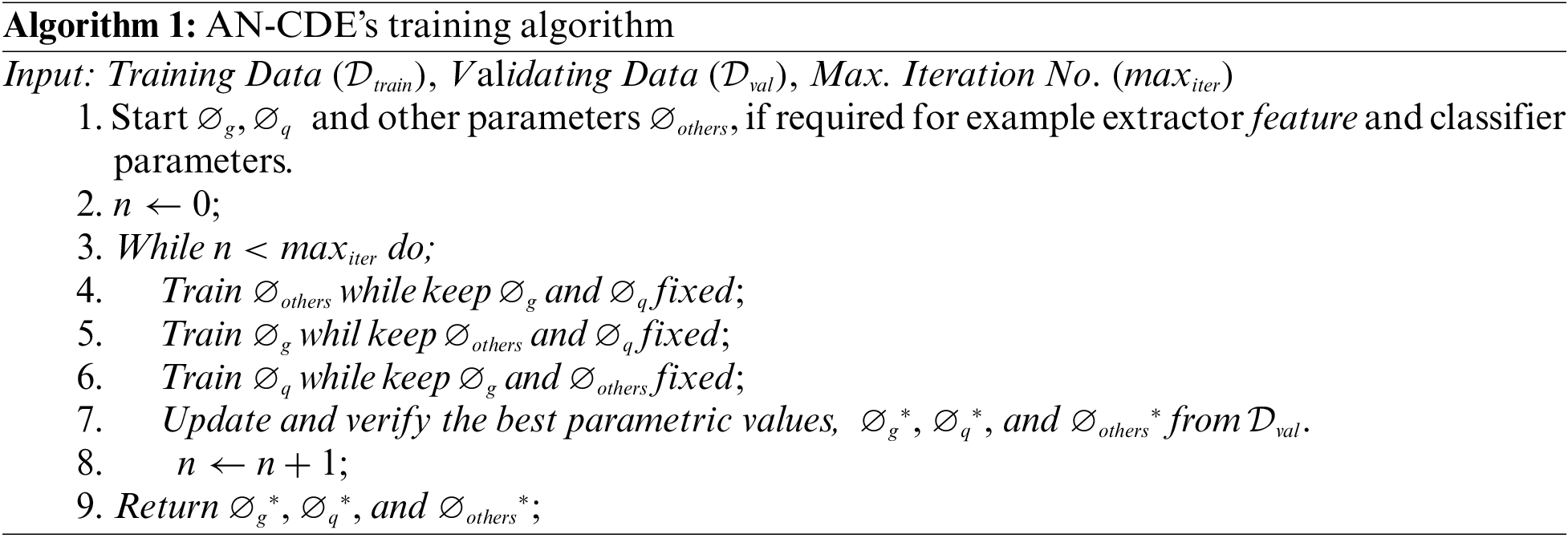
2.5 Training Algorithm and Well-Posedness

Backpropagation adjoint technique is used to trained N-CDE’s whose required memory is O(G+K), where 𝒢=t1−t0 which is referred as integral time space, and 𝓚 denotes size of defined N-CDE’s filed vector. Thus, adjoint method is used in training of Algorithm 1, from Line 4 to 6. Though the proposed algorithm requires two N-CDE’s which results in increment of memory, i.e., O(2𝒢+𝒦g+𝒦q), here 𝒦g and 𝒦q represent the field vector sizes obtained by bottom and top N-CDE’s, respectively.

On a fixed path, the well-posedness of N-CDE’s is already utilizing the mild circumstances of Lipschitz continuity, which have a constant of 1 for all activations including, Softsign, ArcTan, Sigmoid, Tanh, SoftPlus, Leaky ReLU and ReLU. Other commonly used CNN layers, i.e., pooling, batch normalization and dropout have explicit Lipschitz continuity. Thus, the continuity of g and q is achieved in proposed model as the attention values for bottom N-CDE’s are produced by keeping ∅q fixed (Line 5 of Algorithm 1) and attention values for top N-CDE’s re produced by keeping ∅others fixed (Line 6 of Algorithm 1). During the experimental process, the classification task is solved by adopting the ordinary cross entropy loss having a hidden layer w(t) and classification output layer as:

Γo=ς(FCL((w(t))))(19)

Here Γo is the predicted output label and denotes a softmax activations. The output size of FCL is kept uniform equals to total classes in each dataset, whereas standard cross entropy function is also adopted.

3  Experiments

3.1 Datasets and Performance Measures

The proposed model is assessed on two classification tasks (fine-grained visual classification and multi-label classification). A total of five (5) publicly available datasets including are utilized to CUB-200-2011 (D1) and ImageNet-1K (D2), PASCAL VOC 2007 (D3), PASCAL VOC 2012 (D4) and MS COCO (D5) are utilized during the experiments. D3 and D5 are used for multi-label classifications, whereas D1, D2 and D4 are used for fine-grained visual classifications. D1 dataset contains 5994 training and 5794 testing images of bird species. D2 dataset has 1.3 million images for training and 50000 images for testing across 1000 classes. D3 contains 5011 and 4952 images for training and testing across 20 classes, whereas D4 has 11540 training images, 10991 testing images and a total of 20 classes. D5 contains 123000 images and 80 classes, where 82783 are training images and 40504 are testing images.

MaxBoxAccV2 is utilized to evaluate the model on D1 and D2. For D2 and D3, widely used mean Average Precision (mAP) is used along with recording results for each of the 20 classes. Conventional performance measures such as Precision (P), Recall (R), mAP, Average Precision (AvP), Average Recall (AvR), Class-wise Average F1 score (AvF1C) and Overall Average F1 score (AvF1O) are used to evaluate the proposed model on D5.

3.2 Implementation Details

All experiments are performed on Windows 11, Python 3.12.0, CUDA 12.2, TENSORFLOW 2.14.0, MATPLOTLIB 3.8, SCIPY 1.11.3, NUMPY 1.20.3, i7 CPU and NVIDIA RTX TITAN with Nvidia GeForce Graphics Driver 537.58. All experiments are repeated 3 times and reported results are the mean accuracies. For the testing of proposed model on all selected datasets, a total of 240 epochs with a batch size of 16 are executed with {0.5×10−3,2.0×10−3,0.5×10−4,2.0×10−3} learning rate, hidden layers of size {50,60,65,70,75} and N-CDE’s have {6,7,8,9} layers. Best results are achieved by adopting a learning rate of 0.5×10−4, 65 hidden layers and 7 layers in bottom N-CDE’s, whereas 8 layers in top N-CDE’s. When evaluating attention-based models for intra- and inter-class similarities, it is necessary to evaluate the following metrics: F1 score, precision, recall, confusion matrices, and classification accuracy. Furthermore, examining attention maps, ROC curves, AUC, and feature embeddings offers perceptions into the interpretability and performance of the model. While domain-specific metrics take care of application-specific requirements, cross-validation guarantees generality. When these measures are combined with visualization tools, it becomes possible to gain a thorough insight of how well the model handles both intra- and inter-class differences. Standard criteria like classification accuracy, precision, recall, and F1 score are often used in evaluation metrics to examine how well models like N-CDE’s and NODE’s represent similarities and differences. These metrics evaluate the models' capacity to accurately categorize instances, distinguish across classes, and manage variations within a class. Furthermore, based on the particulars of the work, researchers might use more specialized measures, including feature embedding analyses or domain-specific metrics. In order to achieve resilience, the evaluation procedure frequently takes into account the models' performance across different subsets of the data and makes use of cross-validation techniques.

3.3 Comparisons with State-of-the-Art

3.3.1 Results on CUB-200-2011 and ImageNet-1K Dataset

Proposed model is compared with 7 fine-grained image classification methods including iCAM decomposition [21], CREAM [2], WSOL [23], BagCAMs [38], ViTOL [39], iMCL, iMCL [40] and C2AM [24]. This comparison is presented in Table 4. BagCAMs is a plug-and-play technique that was developed for localization task based on the regional localizer generation (RLG) technique, which involves defining a collection of regional localizers and subsequently deriving them from a well-trained classifier. They reported that BagCAMs method achieved SOTA performance on three WSOL benchmarks [38]. Object localization was performed by employing vision transformers for self-attention (ViTOL) and patch-based attention dropout layer (p-ADL) was included to enhance the coverage of the localization map. The results showed that on ImageNet-1K and CUB datasets MaxBoxAcc-V2 localization scores was 70.4% and 73.17%, respectively [39]. Enhancements were introduced to SimCLR by proposing iMCL, where improvements were made in the MoCo framework, accompanied by certain adjustments to MoCo using MLP projection head and the application of additional data augmentation techniques. They established stronger baselines that outperformed SimCLR and do not require large training batches [40]. The proposed model exhibited superior performance compared to iMCL by a margin of 2.3% and outperformed BagCAMs by a margin of 7.3% on the D1 dataset. The performance of the proposed model on the D2 dataset surpasses that of ViTOL and BagCAMs by 5.3% and 5.8%, respectively.

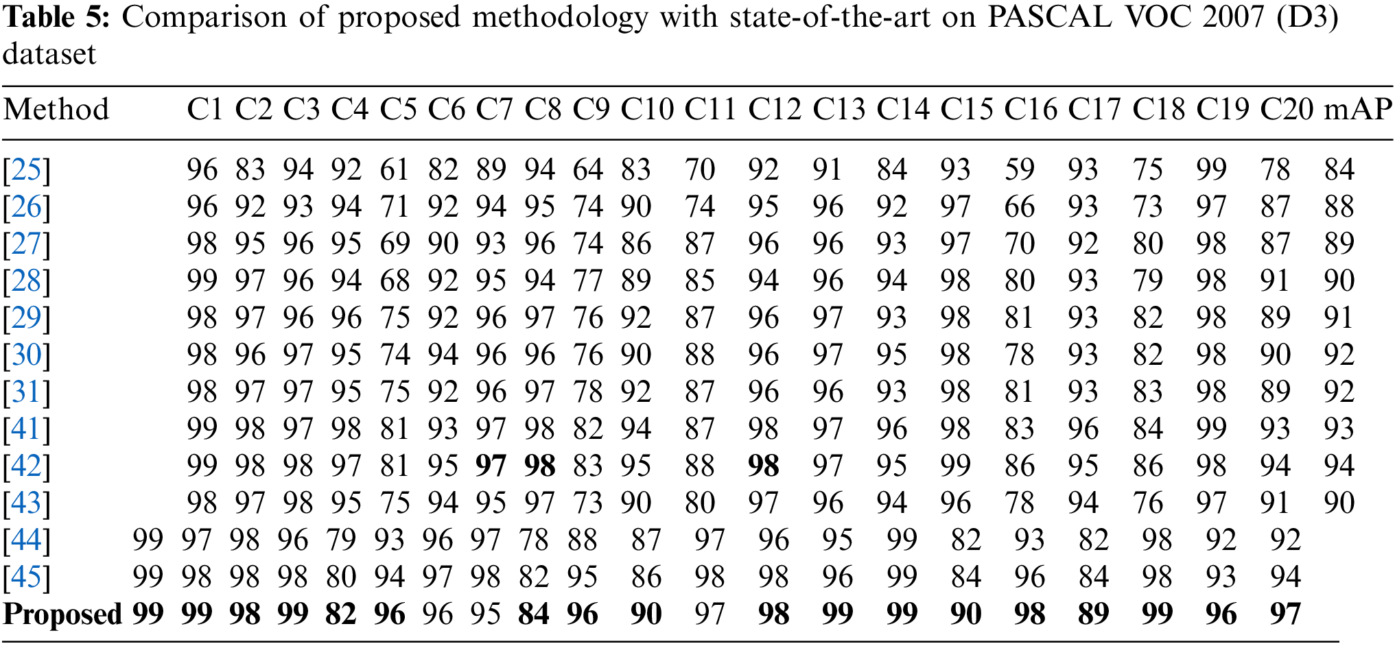
3.3.2 Results on PASCAL VOC 2007 Dataset

For this dataset, the proposed model is compared with 12 models in terms of mAP as shown in Table 5. A simple technique for multi-label classification was designed on the concept of simultaneously recognizing both labels and the correlation of labels utilizing ConvNet and a common latent vector space, respectively. The results demonstrated exceptional performance on MS COCO and PASCAL VOC datasets as benchmark [41]. Deep Semantic Dictionary Learning (DSDL) was developed in which an auto-encoder created the semantic dictionary and then such dictionary was utilized by CNN with label embeddings along with Alternately Parameters Update Strategy (APUS) was applied for training to optimize DSDL. Experimental results showed promising performance on three benchmarks [42]. The proposed model attained a mAP of 97%, surpassing its nearest competitor by a margin of 3%.

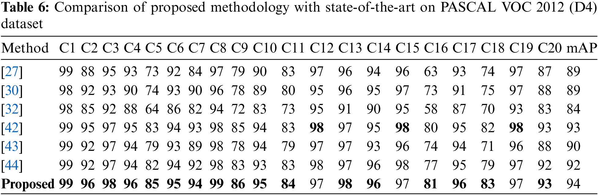
3.3.3 Results on PASCAL VOC 2012 Dataset

The proposed model is compared with 6 latest techniques for this dataset in terms of mAP as shown in Table 6. A deep CNN framework referred to as Hypotheses-CNN-Pooling (HCP) performed classification based on hypotheses extraction, where each supposition is associated to a shared CNN, and the resulting CNN outputs from different suppositions are combined using max pooling. The results demonstrated the superiority of HCP with mAP up to 90.5% [43]. Multi-label image identification employed object-proposal-free framework namely random crop pooling (RCP), which stochastically scales and crops images ahead of delivering them to a CNN. This technique worked well for recognizing the complex innards of multi label images on two datasets, i.e., PASCAL VOC 2012 and PASCAL VOC 2007 [44]. The performance of the proposed model on the D4 dataset surpasses its nearest competitor by a margin of 1%.

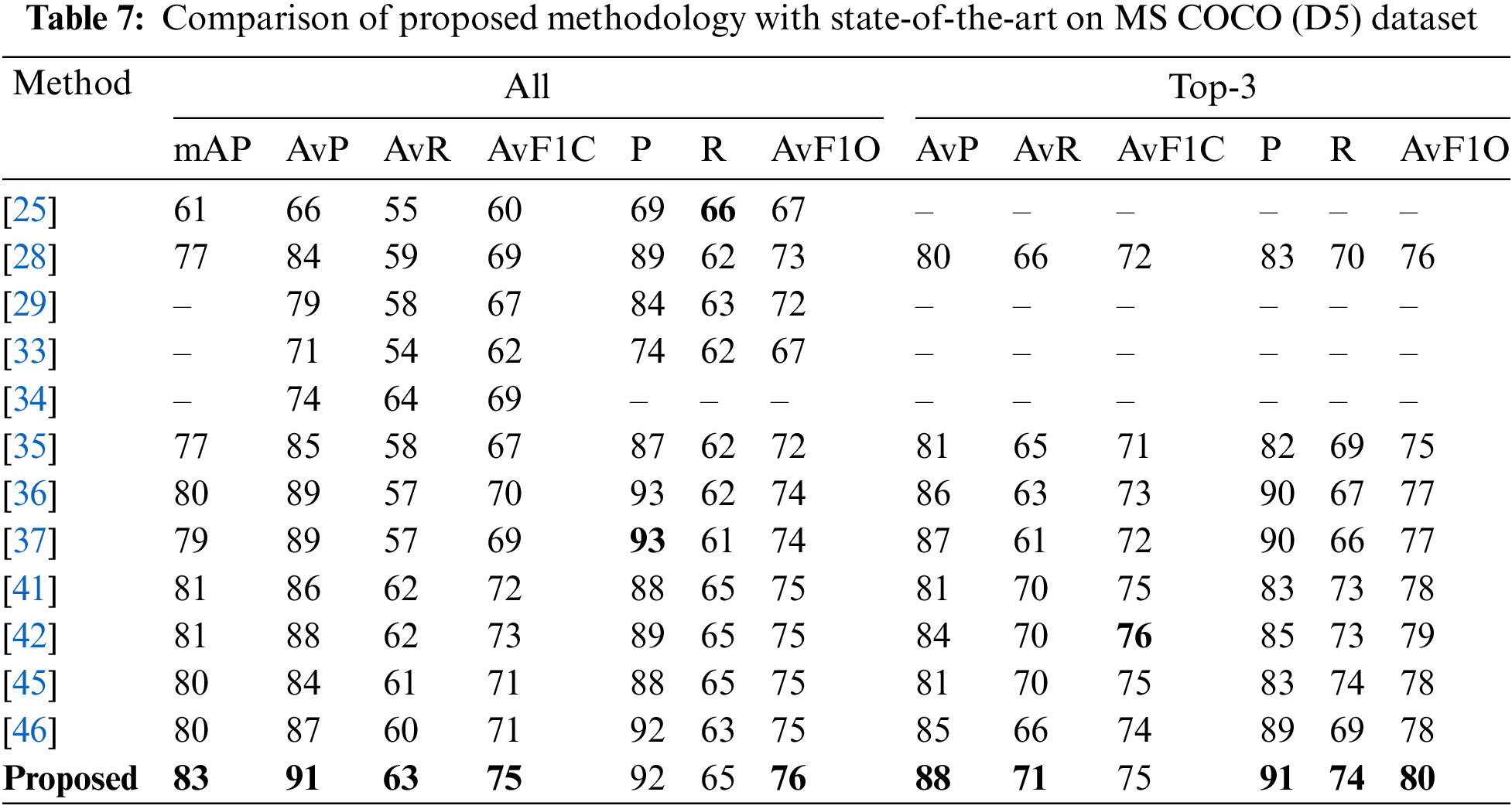
3.3.4 Results on MS COCO Dataset

For this dataset, the proposed model is compared with 12 models as shown in Table 7. The multi label classification model was applied based on graph convolutional network (GCN), where directed graphs were constructed to describe the relationships between object labels, with each label being represented as word embeddings. The GCN was trained to transform this label graph into interdependent object classifiers and represented better performance on two datasets [45]. Efficient Channel Attention (ECA) module achieved improved performance by utilizing a minimal number of parameters. They reported to gain performance boost in terms of Top-1 accuracy of more than 2% [46]. The proposed model performed better than the previous models.

3.4 Visualization of Attention Maps

To visually demonstrate the efficacy of the proposed model in an intuitive and qualitative manner, attention maps are depicted in Fig. 6. The proposed model generates attention maps that are represented by different colors on maps. Dark red indicates the highest level of activation, while dark blue represents the lowest intensity. It is evident that the attention maps for each class effectively identify the object instances that belong to the same class, regardless of the number of objects present in the photos, such as individuals, aircraft, individuals, and animals. Using the final image in the fourth row as a case study, the suggested model effectively demonstrates its ability to accurately identify the position of the penguin, even when the object in question is of diminutive size.

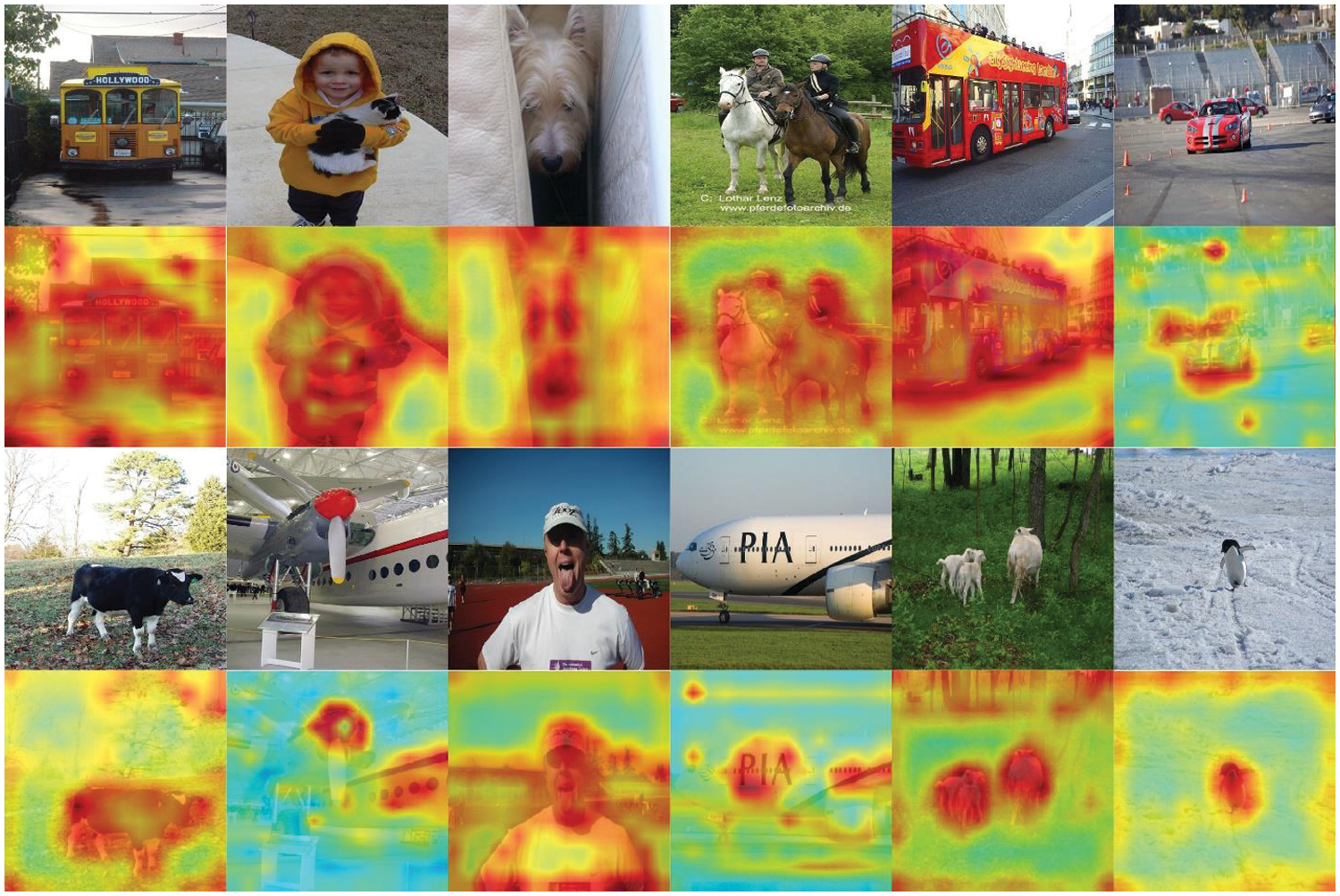
Figure 6: Visualization of attention maps using proposed methodology

The resulting attention maps, which provide a thorough visual examination of the model's decision-making process, are produced by a model that makes use of contextual dense embeddings, or N-CDE’s. These maps provide light on the crucial areas that support the model’s predictions by illustrating where the model focuses its attention within an input. Through close examination of these attention maps, one may identify the locations of relevant regions in the input data, which offers insights into the characteristics that draw the attention of the model. When it comes to tasks like image classification, where certain regions or patterns are suggestive of different classes, this thorough attention analysis is especially helpful. Furthermore, attention maps aid in the recognition of discriminative characteristics, exposing the components that are essential in differentiating between various groups or classifications. This comprehension is further strengthened by the contextual character of N-CDE’s, which demonstrates how the model considers more comprehensive contextual information when making decisions. To put it briefly, attention maps produced by N-CDE’s are an effective instrument for transparent and comprehensible model analysis. They aid in a better understanding of the inner workings of the model and enhance its reliability and performance. Attention-based neural networks using N-CDE’s show potential for NLP, video and image analysis, and medical fields. They promote contextual awareness for better recognition in picture analysis. For more precise predictions, they capture subtle linguistic links in NLP. N-CDE attention models support medical image analysis in the field of healthcare, providing interpretability that is essential for reliable diagnosis. All things considered, N-CDE’s strengthen and dependability of models in a variety of applications.

4  Conclusion

Differential equations have been extensively employed in the context of attention-based classification tasks. Numerous concepts and variants have been presented after the inception of NODE’s, all of which have been constructed upon the fundamental principles of NODE’s. The utilization of NODE's in CNNs has been infrequent, whereas the incorporation of N-CDE’s has been exceedingly rare. This article presents a methodology for generating attention maps using an attentive neural network that utilizes N-CDE’s. The proposed approach involves the use of two distinct types of N-CDE’s: One for incorporating hidden layers and another for generating attention values. The bottom N-CDE’s are employed to capture attention values, while the top N-CDE’s are utilized for the classification task. The proposed approach undergoes evaluation using five publicly available datasets, namely CUB-200-2011, ImageNet-1K, PASCAL VOC 2007, PASCAL VOC 2012, and MS COCO. As all selected datasets contain different types of images, so it was evident that the proposed model is generalized. In the future, the utilization of N-CDE’s can be employed for tasks that necessitate supervised segmentation, particularly in the domains of semantic segmentation and instance segmentation.

Acknowledgement: The author would like to express sincere gratitude to the Department of Information Systems, Faculty of Computing and Information Technology, King Abdulaziz University, Saudi Arabia, for their invaluable support and guidance.

Funding Statement: This research work was funded by Institutional Fund Projects under Grant No. (IFPIP: 638-830-1443). The authors gratefully acknowledge technical and financial support provided by the Ministry of Education and King Abdulaziz University, DSR, Jeddah, Saudi Arabia.

Author Contributions: The authors confirm contribution to the paper as follows: study conception, design, data collection, analysis, interpretation of results and draft manuscript preparation: Anas W. Abulfaraj. The author reviewed the results and approved the final version of the manuscript.

Availability of Data and Materials: The data that support the findings of this study are available from the first and corresponding author upon reasonable request.

Conflicts of Interest: The author declares that they have no conflicts of interest to report regarding the present study.

References

1. M. Raza, J. H. Shah, S. H. Wang, U. Tariq, and M. A. Khan, “HAREDNet: A deep learning based architecture for autonomous video surveillance by recognizing human actions,” Comput. Electr. Eng., vol. 99, no. 1, pp. 107–135, 2022. [Google Scholar]

2. M. Rashid, J. H. Shah, M. Sharif, M. Y. Awan, and M. H. Alkinani, “An optimized approach for breast cancer classification for histopathological images based on hybrid feature set,” Curr. Med. Imag., vol. 17, no. 1, pp. 136–147, 2021. doi: 10.2174/1573405616666200423085826 [Google Scholar] [PubMed] [CrossRef]

3. M. Raza, J. H. Shah, M. A. Khan, and A. Rehman, “Human action recognition using machine learning in uncontrolled environment,” in 2021 1st Int. Conf. Artif. Intell. Data Anal. (CAIDA), Riyadh, Saudi Arabia, 2021, pp. 182–187. [Google Scholar]

4. I. M. Nasir et al., “Improved shark smell optimization algorithm for human action recognition,” Comput. Mater. Contin., vol. 76, no. 3, pp. 2667–2684, 2023. doi: 10.32604/cmc.2023.035214. [Google Scholar] [CrossRef]

5. I. M. Nasir et al., “ENGA: Elastic net-based genetic algorithm for human action recognition,” Expert. Syst. Appl., vol. 227, no. 1, pp. 120–139, 2023. doi: 10.1016/j.eswa.2023.120311. [Google Scholar] [CrossRef]

6. M. A. Khan, M. Yasmin, J. H. Shah, M. Gabryel, and R. Scherer, “Pearson correlation-based feature selection for document classification using balanced training,” Sens., vol. 20, no. 23, pp. 67–83, 2020. [Google Scholar]

7. I. M. Nasir, M. A. Khan, A. Armghan, and M. Y. Javed, “SCNN: A secure convolutional neural network using blockchain,” in 2020 2nd Int. Conf. Comput. Inf. Sci. (ICCIS), Riyadh, Saudi Arabia, 2020, pp. 1–5. [Google Scholar]

8. I. M. Nasir, M. A. Khan, M. Alhaisoni, T. Saba, A. Rehman and T. Iqbal, “A hybrid deep learning architecture for the classification of superhero fashion products: An application for medical-tech classification,” Comput. Model. Eng. Sci., vol. 124, no. 3, pp. 1017–1033, 2020. doi: 10.32604/cmes.2020.010943. [Google Scholar] [CrossRef]

9. T. Lin, M. Maire, S. Belongie, J. Hays, and P. Perona, “Microsoft COCO: Common objects in context,” in Comput. Vis.-ECCV 2014: 13th Eur. Conf., Zurich, Switzerland, 2014, pp. 740–755. [Google Scholar]

10. M. Everingham, L. V. Gool, C. K. Williams, J. Winn, and A. Zisserman, “The pascal visual object classes (VOC) challenge,” Int. J. Comput. Vis., vol. 88, no. 1, pp. 303–338, 2010. doi: 10.1007/s11263-009-0275-4. [Google Scholar] [CrossRef]

11. C. Wah, S. Branson, P. Welinder, P. Perona, and S. Belongie, “The caltech-ucsd birds-200-2011 dataset,” in 13th Eur. Conf., Zurich, Switzerland, 2011, pp. 810–825. [Google Scholar]

12. M. Boukabous and M. Azizi, “Image and video-based crime prediction using object detection and deep learning,” Bull. Electr. Eng. Inform., vol. 12, no. 3, pp. 1630–1638, 2023. doi: 10.11591/eei.v12i3.5157. [Google Scholar] [CrossRef]

13. M. Andronie et al., “Big data management algorithms, deep learning-based object detection technologies, and geospatial simulation and sensor fusion tools in the internet of robotic things,” Isprs. Int. Geo-INF, vol. 12, no. 2, pp. 35–53, 2023. doi: 10.3390/ijgi12020035. [Google Scholar] [CrossRef]

14. C. Moodley, A. Ruget, J. Leach, and A. Forbes, “Time-efficient object recognition in quantum ghost imaging,” Adv. Quantum Technol., vol. 6, no. 2, pp. 109–127, 2023. doi: 10.1002/qute.202200109. [Google Scholar] [CrossRef]

15. S. Rehman, F. Riaz, Q. Saeed, A. Hassan, and M. Khan, “Fully invariant wavelet enhanced minimum average correlation energy filter for object recognition in cluttered and occluded environments,” in Pattern Recognit. Track. XXVIII, California, USA, 2017, pp. 28–39. [Google Scholar]

16. N. Akbar et al., “Detection of moving human using optimized correlation filters in homogeneous environments,” in Pattern Recognit. Track. XXXI, New Mexico, USA, 2020, pp. 73–79. [Google Scholar]

17. Y. Asfia et al., “Selection of CPU scheduling dynamically through machine learning,” in Pattern Recognit. Track. XXXI, New Mexico, USA, 2020, pp. 67–72. [Google Scholar]

18. N. Akbar et al., “Hardware design of correlation filters for target detection,” in Pattern Recognit. Track. XXX, Strasbourg, France, 2019, pp. 71–79. [Google Scholar]

19. Y. Asfia, S. Tehsin, A. Shahzeen, and S. Khan, “Visual person identification device using raspberry Pi,” in 25th Conf. FRUCT Assoc., Maryland, USA, 2019, pp. 422–427. [Google Scholar]

20. S. Saad, A. Bilal, S. Tehsin, and S. Rehman, “Spoof detection for fake biometric images using feature-based techniques,” in SPIE Future Sens. Technol., Yokohama, Japan, 2020, pp. 342–349. [Google Scholar]

21. E. Kim et al., “Bridging the gap between classification and localization for weakly supervised object localization,” in Proc. IEEE/CVF Conf. Comput. Vis. Pattern Recognit., Vancouver, Canada, 2022, pp. 14258–14267. [Google Scholar]

22. J. Xu et al., “CREAM: Weakly supervised object localization via class re-activation mapping,” in Proc. IEEE/CVF Conf. Comput. Vis. Pattern Recognit., New Orleans, USA, 2022, pp. 9437–9446. [Google Scholar]

23. L. Zhu et al., “Weakly supervised object localization as domain adaption,” in Proc. IEEE/CVF Conf. Comput. Vis. Pattern Recognit., Vancouver, Canada, 2022, pp. 14637–14646. [Google Scholar]

24. J. Xie et al., “C2AM: Contrastive learning of class-agnostic activation map for weakly supervised object localization and semantic segmentation,” in Proc. IEEE/CVF Conf. Comput. Vis. Pattern Recognit., New Orleans, USA, 2022, pp. 989–998. [Google Scholar]

25. J. Wang et al., “CNN-RNN: A unified framework for multi-label image classification,” in Proc. IEEE Conf. Comput. Vis. Pattern Recognit., Las Vegas, USA, 2016, pp. 2285–2294. [Google Scholar]

26. J. Zhang, Q. Wu, C. Shen, J. Zhang, and J. Lu, “Multilabel image classification with regional latent semantic dependencies,” IEEE Trans. Multimedia, vol. 20, no. 10, pp. 2801–2813, 2014. doi: 10.1109/TMM.2018.2812605. [Google Scholar] [CrossRef]

27. K. Simonyan and A. Zisserman, “Very deep convolutional networks for large-scale image recognition,” in IEEE Conf. Comput. Vis. Pattern Recognit., Honolulu, USA, 2014, pp. 409–427. [Google Scholar]

28. K. He, X. Zhang, S. Ren, and J. Sun, “Deep residual learning for image recognition,” in Proc. IEEE Conf. Comput. Vis. Pattern Recognit., Las Vegas, USA, 2016, pp. 770–778. [Google Scholar]

29. Z. Wang, T. Chen, G. Li, R. Xu, and L. Lin, “Multi-label image recognition by recurrently discovering attentional regions,” in Proc. IEEE Int. Conf. Comput. Vis., Honolulu, USA, 2017, pp. 464–472. [Google Scholar]

30. H. Yang et al., “Exploit bounding box annotations for multi-label object recognition,” in Proc. IEEE Conf. Comput. Vis. Pattern Recognit., Las Vegas, USA, 2016, pp. 280–288. [Google Scholar]

31. T. Chen, Z. Wang, G. Li, and L. Lin, “Recurrent attentional reinforcement learning for multi-label image recognition,” in Proc. AAAI Conf. Artif. Intell., Washington, USA, 2018, pp. 2018–2035. [Google Scholar]

32. S. He et al., “Reinforced multi-label image classification by exploring curriculum,” in Proc. AAAI Conf. Artif. Intell., Washington, USA, 2018, pp. 285–297. [Google Scholar]

33. S. Chen, Y. Chen, C. Yeh, and Y. Wang, “Order-free RNN with visual attention for multi-label classification,” in Proc. AAAI Conf. Artif. Intell., Washington, USA, 2018, pp. 2175–2187. [Google Scholar]

34. C. Lee, W. Fang, C. Yeh, and Y. Wang, “Multi-label zero-shot learning with structured knowledge graphs,” in Proc. IEEE Conf. Comput. Vis. Pattern Recognit., Salt Lake City, USA, 2018, pp. 1576–1585. [Google Scholar]

35. F. Zhu et al., “Learning spatial regularization with image-level supervisions for multi-label image classification,” in Proc. IEEE Conf. Comput. Vis. Pattern Recognit., Honolulu, USA, 2017, pp. 5513–5522. [Google Scholar]

36. S. Woo, J. Park, J. Lee, and I. Kweon, “CBAM: Convolutional block attention module,” in Proc. Eur. Conf. Comput. Vis., Tel Aviv, Israel, 2018, pp. 3–19. [Google Scholar]

37. J. Hu, L. Shen, and G. Sun, “Squeeze-and-excitation networks,” in Proc. IEEE Conf. Comput. Vis. Pattern Recognit., Salt Lake City, USA, 2018, pp. 7132–7141. [Google Scholar]

38. L. Zhu et al., “Bagging regional classification activation maps for weakly supervised object localization,” in Eur. Conf. Comput. Vis., Tel Aviv, Israel, 2022, pp. 176–192. [Google Scholar]

39. S. Gupta, S. Lakhotia, A. Rawat, and R. Tallamraju, “ViTOL: Vision transformer for weakly supervised object localization,” in Proc. IEEE/CVF Conf. Comput. Vis. Pattern Recognit., New Orleans, USA, 2022, pp. 4101–4110. [Google Scholar]

40. X. Chen, H. Fan, R. Girshick, and K. He, “Improved baselines with momentum contrastive learning,” in IEEE/CVF Conf. Comput. Vis. Pattern Recognit., Seattle, USA, 2020, pp. 3514–3526. [Google Scholar]

41. S. Wen et al., “Multilabel image classification via feature/label co-projection,” IEEE Trans. Syst. Man Cybern.: Syst., vol. 51, no. 11, pp. 7250–7259, 2020. doi: 10.1109/TSMC.2020.2967071. [Google Scholar] [CrossRef]

42. F. Zhou, S. Huang, and Y. Xing, “Deep semantic dictionary learning for multi-label image classification,” in Proc. AAAI Conf. Artif. Intell., Washington, USA, 2021, pp. 3572–3580. [Google Scholar]

43. Y. Wei et al., “HCP: A flexible CNN framework for multi-label image classification,” IEEE Trans. Pattern Anal. Mach. Intell., vol. 38, no. 9, pp. 1901–1907, 2015. doi: 10.1109/TPAMI.2015.2491929 [Google Scholar] [PubMed] [CrossRef]

44. M. Wang, C. Luo, R. Hong, J. Tang, and J. Feng, “Beyond object proposals: Random crop pooling for multi-label image recognition,” IEEE Trans. on Image Process., vol. 25, no. 12, pp. 5678–5688, 2016. doi: 10.1109/TIP.2016.2612829 [Google Scholar] [PubMed] [CrossRef]

45. Z. Chen, X. Wei, P. Wang, and Y. Guo, “Multi-label image recognition with graph convolutional networks,” in Proc. IEEE/CVF Conf. Comput. Vis. Pattern Recognit., Long Beach, USA, 2019, pp. 5177–5186. [Google Scholar]

46. Q. Wang et al., “ECA-Net: Efficient channel attention for deep convolutional neural networks,” in Proc. AAAI Conf. Artif. Intell., Washington, USA, 2020, pp. 11534–11542. [Google Scholar]