A Spectral Convolutional Neural Network Model Based on Adaptive Fick’s Law for Hyperspectral Image Classification

1  Introduction

Hyperspectral images (HSIs) have found extensive applications in various fields such as remote sensing, establishing themselves as a focal point within the remote sensing domain [1–3]. In addition to spatial resolution, HSIs possess spectral resolution [4]. The acquisition of HSIs originates from diverse hyperspectral sensors, which capture tens to hundreds of spectral bands. While obtaining surface image information, these sensors also acquire spectral information, representing a fusion of spectral and imaging data [5]. HSIs can be used for land classification, which can distinguish different types of objects and cover on the surface. By analyzing spectral features, accurate classification of vegetation types, buildings, and other targets can be achieved.

With the advancement of remote sensing technology, the acquisition of hyperspectral image data has significantly increased. These datasets typically encompass hundreds or even thousands of spectral bands. Traditional image processing and classification techniques have proven insufficient in effectively addressing the challenges, thus leading to the gradual emergence of machine learning and deep learning into our purview [6,7]. Models such as Random Forests, K-Nearest Neighbors (KNN), and Support Vector Machines (SVM), among others, have been widely utilized for HSI classification [8,9]. Among these, SVM has gained extensive application, resulting in numerous variations. For instance, Okwuashi and Ndehedehe [10] presented the Deep Support Vector Machine (DSVM), employing four distinct kernel functions within the DSVM framework.

With the continuous advancement of deep learning, an increasing number of researchers have been employing neural networks for HSI classification [11]. In 2020, Hong et al. [12] introduced a novel mini-batch Graph Convolutional Network (miniGCN) to address HSI classification issues, demonstrating the superior performance of the miniGCN model over CNN and GCN models. In 2021, Ghaderizadeh et al. [13] utilized a hybrid 3D-2D CNN for HSI classification, illustrating the superior performance of the hybrid CNN model compared to 2D-CNN and 3D-CNN models. Subsequently, in 2022, Jia et al. [14] proposed a Graph-in-Graph Convolutional Network (GiGCN) for HSI classification, demonstrating its efficacy in HSI classification tasks through experimental validation. Finally, in 2023, Ge et al. [15] introduced a dual-branch convolutional neural network equipped with polarized self-attention mechanism to investigate HSI classification problems, validating the effectiveness of the proposed network across multiple public datasets.

Despite the utilization of advanced neural network technologies in recent studies, the selection of neural network hyperparameters involves a certain degree of empiricism and randomness. To identify the most suitable hyperparameters, researchers have begun integrating intelligent optimization algorithms with neural networks [16]. After recent years of research, intelligent optimization algorithms have developed rapidly [17–20]. In 2020, Banadkooki et al. [21] combined Artificial Neural Networks (ANN) with ALO, BA, and PSO to establish ANN-ALO, ANN-BA, and ANN-PSO models for the prediction of suspended sediment load. In 2021, Nikbakht et al. [22] applied a Genetic Algorithm to neural networks to discover optimal hyperparameter values, demonstrating its effectiveness in engineering problems. In 2022, Fan et al. [23] introduced a novel Hybrid Sparrow Search Algorithm (HSSA) to address hyperparameter optimization in models, with experimental results confirming the method’s efficacy. In 2023, Falahzadeh et al. [24] proposed a model combining Deep Convolutional Neural Networks with Grey Wolf Optimization (GWO) to optimize neural network hyperparameters. Through numerous studies, it is evident that intelligent optimization algorithms can effectively optimize neural network hyperparameters.

The Fick’s Law algorithm (FLA) was proposed by Hashim et al. [25] in 2022, which is a novel intelligent optimization algorithm. The inspiration for this algorithm comes from Fick’s law in physics. After a year of research, improvements to the Fick’s Law algorithm have been gradually proposed. Alghamdi et al. [26] improved the FLA using Rosenbrock’s direct rotation method and applied the improved FLA to the scheduling and management of the energy hub. Mehta et al. [27] improved the FLA using a quasi-oppositional-based approach and applied the improved FLA to mechanical design problems. However, these improved Fick’s Law algorithms cannot adjust weights based on changes in the number of iterations, making our research particularly important.

To enhance the accuracy of HSI classification and improve the performance of neural networks, we propose a Spectral Convolutional Neural Network model based on Adaptive Fick’s Law Algorithm (AFLA-SCNN). This model utilizes the AFLA to optimize two hyperparameters within the SCNN, thereby enhancing the performance of SCNN and consequently improving the accuracy of HSI Classification. The primary contributions of this paper are outlined as follows:

1.    Introduction of the Adaptive Fick’s Law Algorithm (AFLA) as an improved version of the FLA. AFLA incorporates three novel strategies: Adaptive weight factor, Gaussian mutation, and probability update policy. Moreover, comparative experiments were carried out between AFLA and nine widely recognized intelligent optimization algorithms utilizing the CEC2013 and CEC2017 datasets.

2.    Proposal of the Spectral Convolutional Neural Network model based on Adaptive Fick’s Law Algorithm (AFLA-SCNN). This model employs AFLA to optimize two hyperparameters, “numEpochs” and “miniBatchSize”, within SCNN. Upon obtaining the optimal parameter values, they are input into SCNN for HSI classification. Additionally, comparative experiments were conducted among AFLA-SCNN, FLA-SCNN, HHO-SCNN, DE-SCNN, SCNN, and SVM models utilizing the Indian Pines dataset and Pavia University dataset.

The structure of this paper is outlined as follows: Section 2 introduces the relevant work on FLA and SCNN. Section 3 details AFLA and provides pseudocode. Section 4 elaborates on the construction and detailed workflow of the AFLA-SCNN model. Section 5 conducts performance verification experiments on AFLA. Section 6 assesses the performance of the AFLA-SCNN model in HSI classification. The final section summarizes the entire paper.

2  Related Work

2.1 Fick’s Law Algorithm (FLA)

The inspiration for FLA is derived from Fick’s law, which is a fundamental physical law [28]. The mathematical expression of Fick’s law is:

J=−DdCdx(1)

In Eq. (1), J is the diffusion flux per unit area per unit time, D is the diffusion coefficient, and dCdx is the concentration gradient per unit area. FLA has three stages: DO (diffusion operator), EO (equilibrium operator), and SSO (steady-state operator).

2.1.1 DO

Eqs. (2)–(4) are used to control the direction of molecular movement, where Xmt represents the position of molecule m, R represents a random number, and C1 is a constant equal to 5.

TDOt=C2×TFt−R,C2=2(2)

TFt=sinh(tT)C1(3)

Xmt={ from region i to region jTDOt<Rfrom region j to region iotherwise(4)

First describe the case where the concentration in region i is greater than that in region j, in which case the molecular formula from i to j is:

Xij,mt+1=Xj,bestt+DFijt×R×DOFt×(Jij,mt×Xj,bestt−Xij,mt)(5)

where Xj,bestt represents the optimal position in region j, DFijt is −1 or 1, and DOFt is calculated by:

DOFt=exp(−C5×(TFt−R)),C5=2(6)

C5 is a constant equal to 2. Additionally, Jij,mt is calculated by:

Jij,mt=−DdCijtdxij,mt(7)

where D is 0.01, and dCijt and dxij,mt are as follows:

dCijt=Xj,meant−Xi,meant(8)

dxij,mt=(Xj,beatt)2−(Xij,mt)2+eps(9)

The remaining molecules in region i can be updated in three different ways, which are calculated using the following formulas:

Xi,mt+1={Xi,bestt0<R<0.8Xi,bestt+DOFt×(L+R×(U−L))0.8≤R<0.9Xi,mtotherwise(10)

If region j has a higher concentration than region i, one can interchange i and j in the aforementioned process.

2.1.2 EO

In this stage, we will focus on the updates for groups g1 and g2. The group g1 is as follows:

Xg1,mt+1=Xg1,bestt+Qg1,mt×Xg1,mt+Qg1,mt×(MSg1,mt×Xg1,bestt−Xg1,mt)(11)

where Qg1,mt is as follows:

Qg1,mt=R×DFg1t×DRFg1,mt(12)

DRFg1,mt=exp(−Jg1,mtTFt)(13)

The Jg1,mt is as follows:

Jg1,mt=−DdCg1tdxg1,mt(14)

dCg1t=Xg1,bestt−Xg1,meant(15)

dxg1,mt=(Xg1,bestt)2−(Xg1,mt)2+eps(16)

Additionally, MSg1,mt is as follows:

MSg1,mt=exp(−FSg1,besttFSg1,mt+eps)(17)

Among them, FSg1,bestt and FSg1,mt represent the best fitness value in g1 and the fitness value of molecule m in g1, respectively.

Therefore, to update formulas for group g2, simply replace g1 with g2 in the above process.

2.1.3 SSO

The group g1 is as follows:

Xg1,mt+1=Xbestt+Qg1,mt×Xg1,mt+Qg1,mt×(MSg1,mt×Xbestt−Xg1,mt)(18)

In Eq. (18), Qg1,mt is calculated using the Eqs. (12)–(14). The dCg1t and dxg1,mt are modified to:

dCg1t=Xg1,meant−Xbestt(19)

dxg1,mt=(Xbestt)2−(Xg1,mt)2+eps(20)

Moreover, the MSg1,mt is modified to:

MSg1,mt=exp(−FSbesttFSg1,mt+eps)(21)

Therefore, to update formulas for group g2, simply replace g1 with g2 in the above process.

2.2 Spectral Convolution Neural Network (SCNN)

Spectral Convolutional Neural Network (SCNN) has become a powerful tool for image processing and analysis, especially in processing spectral information [29]. Unlike traditional convolutional neural networks that mainly focus on the spatial relationships between pixels, SCNN considers both spatial and spectral relationships, providing a more comprehensive understanding of image content [30]. Especially hyperspectral images, due to their high dimensionality and complexity, pose unique challenges. These images are composed of many bands, each with different spectral features, reflecting the characteristics of different materials and features in the scene [31]. Traditional image processing methods often struggle to effectively capture and utilize this spectral information, but SCNN is specifically designed to handle this complexity. This spectral-spatial fusion allows the network to extract meaningful features from the spatial layout of pixels and the spectral features they emit. Therefore, SCNN is very effective in tasks such as classification, recognition, and segmentation [32].

In summary, spectral convolutional neural networks have significant advantages in processing and analyzing hyperspectral images and spectral data. By considering the spatial and spectral relationships between pixels, they can extract more comprehensive and meaningful features from the data. This spectral-spatial fusion not only improves the accuracy and precision of classification and recognition tasks, but also opens up new possibilities for advanced image processing and analysis applications in a wide range of fields such as remote sensing, environmental monitoring, and medical imaging.

In this paper, the SCNN structure depicted in Fig. 1 is utilized. The SCNN has seventeen layers of structure, the first layer is a 3D image input layer, the input size is 25 × 25 × 30. The second layer is a 3D convolutional layer, the size is 3 × 3 × 7 and the number is 8. The third layer is a ReLU layer. The fourth layer is a 3D convolutional layer, the size is 3 × 3 × 5 and the number is 16, The fifth layer is a ReLU layer. The sixth layer is a 3D convolutional layer with size 3 × 3 × 3 and number 32. The seventh layer is a ReLU layer. The eighth layer is a 3D convolutional layer with size 3 × 3 × 1 and number 8. The ninth layer is a ReLU layer. The tenth layer is a fully-connected layer with an output size of 256. The eleventh layer is a ReLU layer. The twelfth layer is a discard layer with probability of 0.4. The thirteenth layer is a fully-connected layer with an output size of is 128. The fourteenth layer is the discard layer with a probability of 0.4. The fifteenth layer is the fully connected layer with an output size of 16. The sixteenth layer is the Softmax layer, and the seventeenth layer is the output layer.

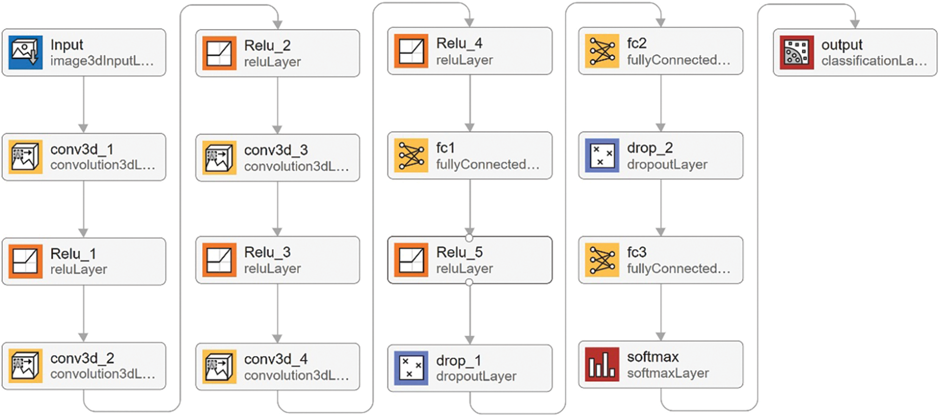
Figure 1: Structure of SCNN

3  Adaptive Fick’s Law Algorithm (AFLA)

The initial FLA was considered to have limitations, mainly due to its tendency to fall into local optima and converge prematurely before reaching the global optimal solution. These issues may lead to suboptimal results and limit the effectiveness of algorithms in complex optimization problems. Solving these issues is crucial for improving the performance and reliability of FLA.

In this paper, we introduce an enhanced version of FLA called AFLA. AFLA addresses the limitations of the initial FLA by combining three innovative strategies. Firstly, an adaptive weight factor is introduced. This factor dynamically adjusts weights based on the progress of the optimization process. By doing so, AFLA can better balance the exploration and utilization of search space, reducing the chances of falling into local optima. Secondly, integrate Gaussian variation into AFLA. This mutation strategy introduces random perturbations into the current solution, allowing the algorithm to escape from the local optimal region. The Gaussian mutation is carefully designed to maintain a balance between exploration and development, ensuring that the search remains focused while still exploring promising areas. Finally, adopt a probability update strategy. This strategy adjusts the probability associated with different fuzzy rules based on their historical performance. By doing so, AFLA can shift its search towards more successful rules, thereby accelerating the convergence process.

In summary, these three strategies aim to enhance the exploration and development capabilities of FLA, addressing its tendency to fall into local optima and premature convergence [33–35]. By combining these strategies, AFLA is expected to demonstrate excellent performance in complex optimization problems and provide more accurate and reliable solutions.

3.1 Adaptive Weight Factor

To improve the algorithm’s local search capability, an adaptive weight factor denoted as ω has been introduced. The formula for calculating the adaptive weight factor ω is depicted in Eq. (22).

ω=rand×(1−tT)(22)

At the beginning of the iteration, ω will take random values within the range (0, 1), and as the number of iterations increases, the range of values will gradually decrease. The calculated values of ω when T=1000 have been presented in a curve graph, as depicted in Fig. 2.

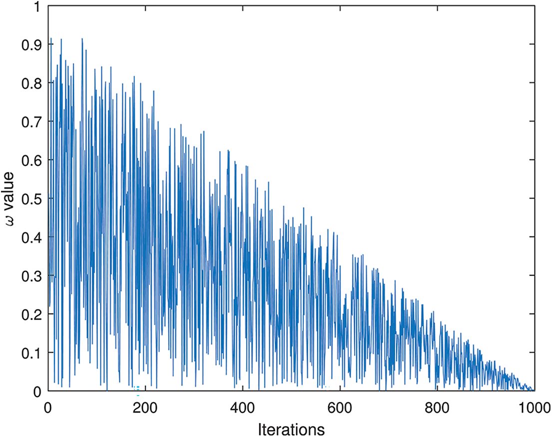
Figure 2: Variation of ω with Iterations as T=1000

We have ω into the position update formulas for the DO phase, resulting in Eqs. (5) and (10) being transformed to:

Xij,mt+1=Xj,bestt+DFijt×ω×(Jij,mt×Xj,bestt−Xij,mt)(23)

Xi,mt+1={ Xi,bestt0<rand<0.8Xi,bestt+ω×(L+rand×(U−L))0.8≤rand<0.9Xi,mtotherwise(24)

3.2 Gaussian Mutation

The Gaussian mutation is as follows:

G=1σ2πe−(x−μ)22σ2(25)

In this paper, we set μ to 0 and σ to 1, respectively, and select x as a random number within the range of (0, 3).

We introduce Gaussian mutation into the position update formulas for the DO, EO, and SSO phases, resulting in Eqs. (5), (11), and (18) being transformed to:

Xij,mt+1=Xj,bestt+DFijt×ω×(Jij,mt×Xj,bestt−Xij,mt)+G×Xij,mt(26)

Xg1,mt+1=Xg1,bestt+Qg1,mt×Xg1,mt+Qg1,mt×(MSg1,mt×Xg1,bestt−Xg1,mt)+G×Xij,mt(27)

Xg1,mt+1=Xbestt+Qg1,mt×Xg1,mt+Qg1,mt×(MSg1,mt×Xbestt−Xg1,mt)+G×Xij,mt(28)

3.3 Probability Update Strategy

In order to improve the algorithm’s local search and to prevent the algorithm from getting stuck in local optima, we have introduced a probability update strategy. In the DO phase, both the update formulas for the remaining molecules in region i, resulting in Eq. (10) being transformed to:

Xi,mt+1={ Xi,besttXi,bestt+ω×(L+rand×(U−L)) 0<rand<0.8otherwise(29)

4  Proposed AFLA-SCNN Model

To enhance the accuracy of HSI classification, we proposed the Adaptive Feichtinger’s Law Algorithm (AFLA) and applied it to optimize the hyperparameters of the spectral convolutional neural network (SCNN). Consequently, we introduced a Spectral Convolutional Neural Network model based on the Adaptive Feichtinger’s Law Algorithm (AFLA-SCNN). Within this model, AFLA dynamically adjusts weights based on the iteration count, enabling it to obtain the optimal hyperparameters for SCNN.

Specifically, we employed AFLA to optimize the hyperparameters “numEpochs” and “miniBatchSize” within SCNN, acquiring their optimal values through AFLA. “numEpochs” represents the total number of training iterations or the number of times the model traverses the dataset. Excessively large “numEpochs” may lead to overfitting, where the model excels on training data but performs poorly on new, unseen data. Conversely, too few “numEpochs” may result in underfitting, causing inadequate exploration of the training data’s features and patterns. “miniBatchSize” refers to the number of samples used for weight updates during each iteration. In our model, we utilized a technique called “batch gradient descent,” which updates weights using a subset of training samples rather than the entire training set. Oversized “miniBatchSize” might slow down training, while a smaller “miniBatchSize” could lead to training instability or suboptimal model performance. Thus, selecting appropriate values for “numEpochs” and “miniBatchSize” is crucial within the network model [36–38].

The flowchart of AFLA-SCNN is depicted in Fig. 3. In this figure, the AFLA-SCNN model is divided into two parts, with the flow of AFLA on the left and the flow of SCNN within the dashed line on the right. When calculating the fitness value of each solution in AFLA, the SCNN model is invoked, and the complement number of accuracy in the SCNN model is used as the fitness value of each solution in AFLA. Subsequently, the model calculates the TF value and calls for different optimization methods based on the TF value. Then, the fitness value is calculated again. The result is output after the maximum number of iterations is reached. A detailed description of the process follows below:

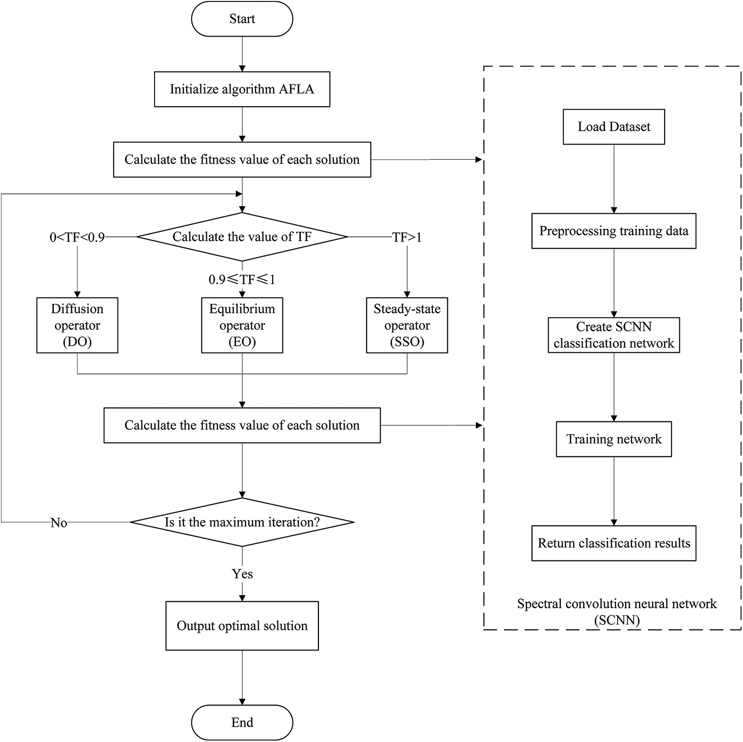
Figure 3: The flowchart of the AFLA-SCNN model

1.    Initialize algorithm AFLA. Initialize the number of solutions to be computed, the number of iterations, dimensions, and upper and lower bounds for AFLA.

2.    Compute the fitness value for each solution. Invoke the SCNN network, load the dataset, preprocess the training data, create the SCNN classification network, train the network, and finally obtain the classification accuracy. Set the fitness value as the complement number of the accuracy achieved by the SCNN network.

3.    Compute the value of TF. If 0<TF<0.9, proceed to the diffusion operator; if 0.9≤TF≤1, proceed to the equilibrium operator; if TF>1, proceed to the steady-state operator.

4.    Recalculate the fitness value for each solution. Again, invoke the SCNN network.

5.    Check if it is the maximum iteration count. If it is not the maximum iteration count, return to Step 3; if it is the maximum iteration count, output the best solution.

5  Performance Validation Experiment of AFLA

In this section, we validate the performance of AFLA through experiments on benchmark functions from CEC2013 and CEC2017 [39,40]. Additionally, we compared AFLA with the original FLA and several well-known metaheuristic algorithms.

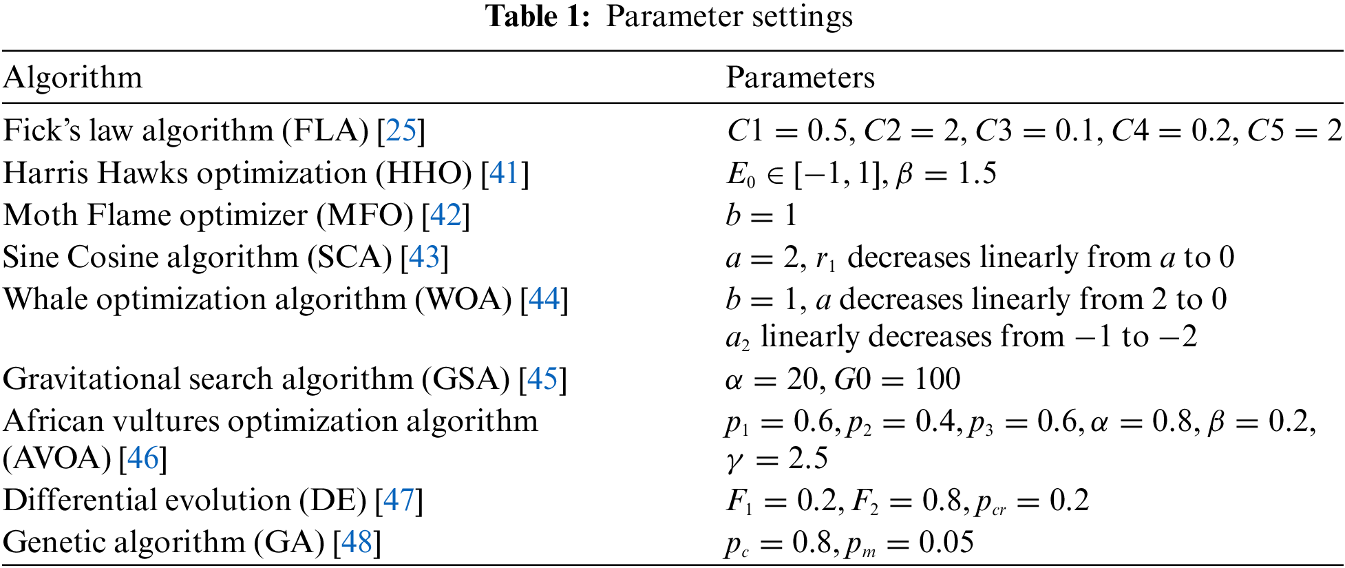
To ensure fair and just comparison between different algorithms, we standardized the experimental settings of all algorithms involved in the study. Specifically, we set the overall size of all algorithms (representing the number of particles or populations participating in the optimization process) to 50. This ensures that it is relatively unaffected by differences in population size. In addition, we will limit the maximum number of iterations to 1000. This limitation means that each algorithm has a fixed number of opportunities to search for the optimal solution, ensuring the fairness of the computing resources used. To define the search space, we set the lower limit of the search range to −100 and the upper limit to 100. These boundaries represent the minimum and maximum values that the algorithm can explore during the optimization process. By setting the same boundaries for all algorithms, we ensure that they run in the same search space for direct comparison. For other parameter settings, as shown in Table 1, Table 1 provides a detailed list of specific parameter values for each algorithm. These parameter values are selected based on generally accepted values in the literature or through preliminary experiments to ensure optimal performance. To further ensure the reliability of the results, we ran each algorithm multiple times. Specifically, we will run each algorithm 50 times and compare the best fitness values obtained during these runs. The optimal fitness value refers to the lowest fitness value obtained in 50 runs, as in intelligent optimization problems, the goal is usually to minimize the fitness value. By comparing the optimal fitness values of multiple runs, we can consider any potential anomalies or fluctuations in algorithm performance.

5.1 Experiments on CEC2013

In this section, we will evaluate the proposed AFLA within the CEC2013 dataset. CEC2013 comprises 28 functions [49]. After adjusting the objective values of all functions to zero, we will conduct comparative experiments by evaluating AFLA and nine other algorithms across dimensions of 10D, 30D, and 50D.

5.1.1 Result of 10D

Table 2 shows the performance of AFLA and nine other algorithms on the 10D benchmark functions of CEC2013. In this table, the symbol “+” means that AFLA outperforms the respective algorithm, “≈” signifies AFLA performs comparably to the algorithm, and “−” indicates AFLA performs worse than the algorithm. The last row of the table exhibits the statistics for each algorithm across the 28 functions.

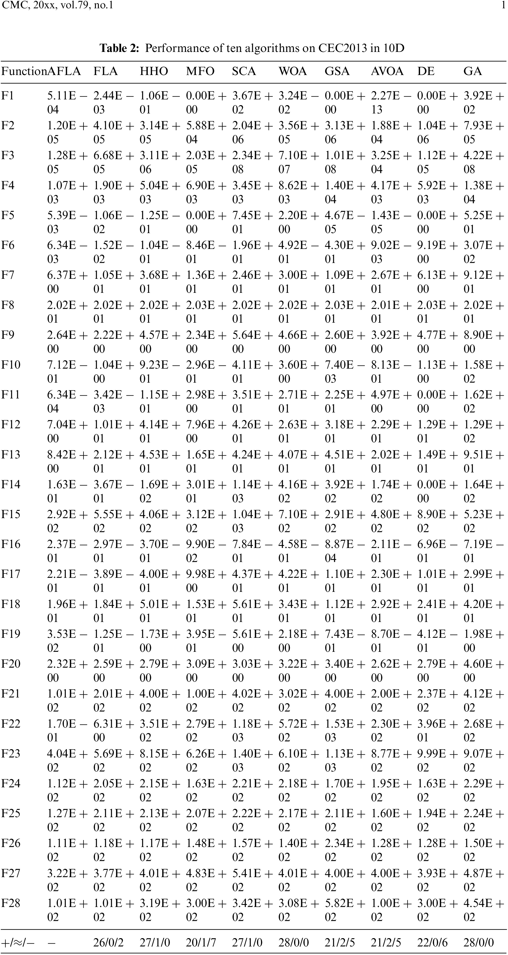
From Table 2, it is evident that AFLA surpasses FLA in 26 functions, outperforms HHO in 27 functions, exceeds MFO in 20 functions, outshines SCA in 27 functions, prevails over WOA in all 28 functions, surpasses GSA in 21 functions, outperforms AVOA in 21 functions, performs better than DE in 22 functions, and outperforms GA in all 28 functions. Finally, we assert that AFLA demonstrates commendable performance across the 28 functions of CEC2013 in 10D.

5.1.2 Result of 30D

The performance of AFLA and nine comparative algorithms on the benchmark functions of CEC2013 in 30D is presented in Table 3.

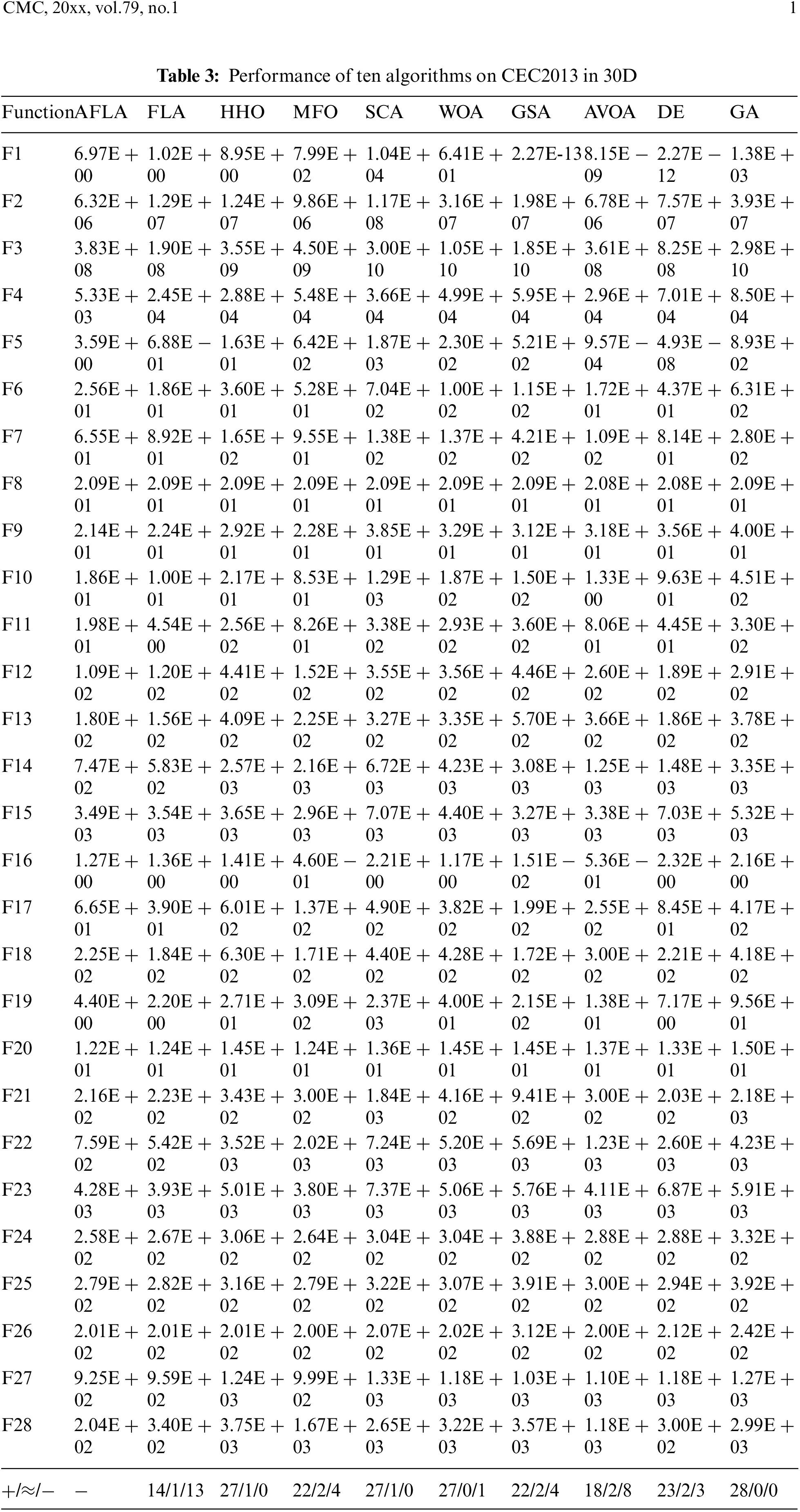
From Table 3, it shows that AFLA surpasses FLA in 14 functions, outperforms HHO in 27 functions, exceeds MFO in 22 functions, outshines SCA in 27 functions, prevails over WOA in all 27 functions, surpasses GSA in 22 functions, performs better than AVOA in 18 functions, outperforms DE in 23 functions, and outperforms GA in all 28 functions. Finally, we assert that AFLA demonstrates commendable performance across the 28 functions of CEC2013 in 30D.

5.1.3 Result of 50D

The performance of AFLA and nine comparative algorithms on the 50D benchmark functions of CEC2013 is presented in Table 4.

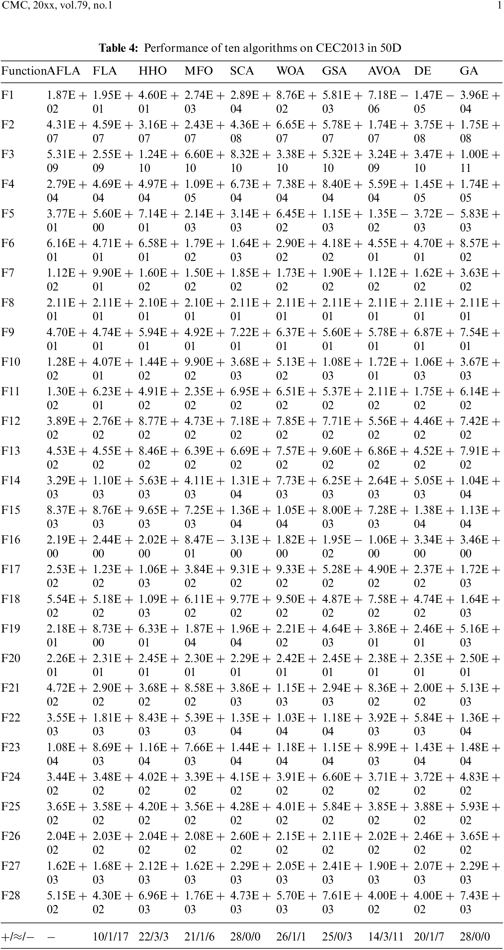
From Table 4, it is evident that AFLA outperforms FLA in 10 functions, surpasses HHO in 22 functions, exceeds MFO in 21 functions, outshines SCA in 28 functions, surpasses WOA in 26 functions, performs better than GSA in 25 functions, outperforms AVOA in 14 functions, exceeds DE in 20 functions, and outperforms GA in all 28 functions. Finally, we assert that AFLA demonstrates commendable performance across the 28 functions of CEC2013 in 50D.

5.2 Experiments on CEC2017

In this section, we will evaluate the proposed AFLA within the CEC2017 dataset. CEC2017 comprises 29 functions [50]. After adjusting the objective values of all functions to zero, we will conduct comparative experiments by evaluating AFLA and nine other algorithms across dimensions of 10D, 30D, and 50D.

5.2.1 Result of 10D

The performance of AFLA and nine comparative algorithms on the benchmark functions of CEC2017 in 10D is presented in Table 5.

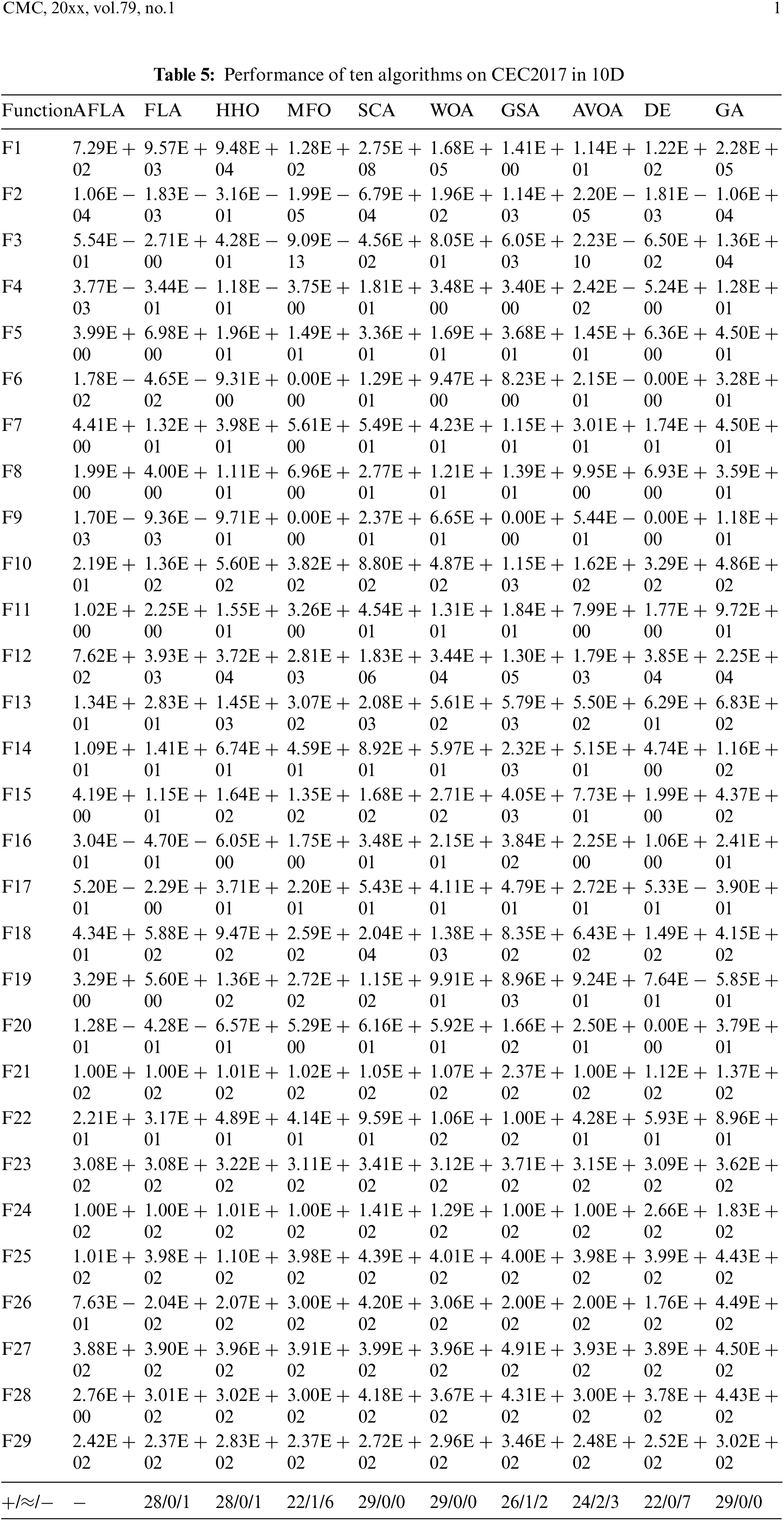
From Table 5, it is evident that AFLA outperforms FLA in 28 functions, surpasses HHO in 28 functions, exceeds MFO in 22 functions, outshines SCA in all 29 functions, surpasses WOA in all 29 functions, performs better than GSA in 26 functions, outperforms AVOA in 24 functions, exceeds DE in 22 functions, and outperforms GA in all 29 functions. In conclusion, we assert that AFLA demonstrates commendable performance across the 29 functions of CEC2017 in 10D.

5.2.2 Result of 30D

The performance of AFLA and nine comparative algorithms on the benchmark functions of CEC2017 in 30D is presented in Table 6.

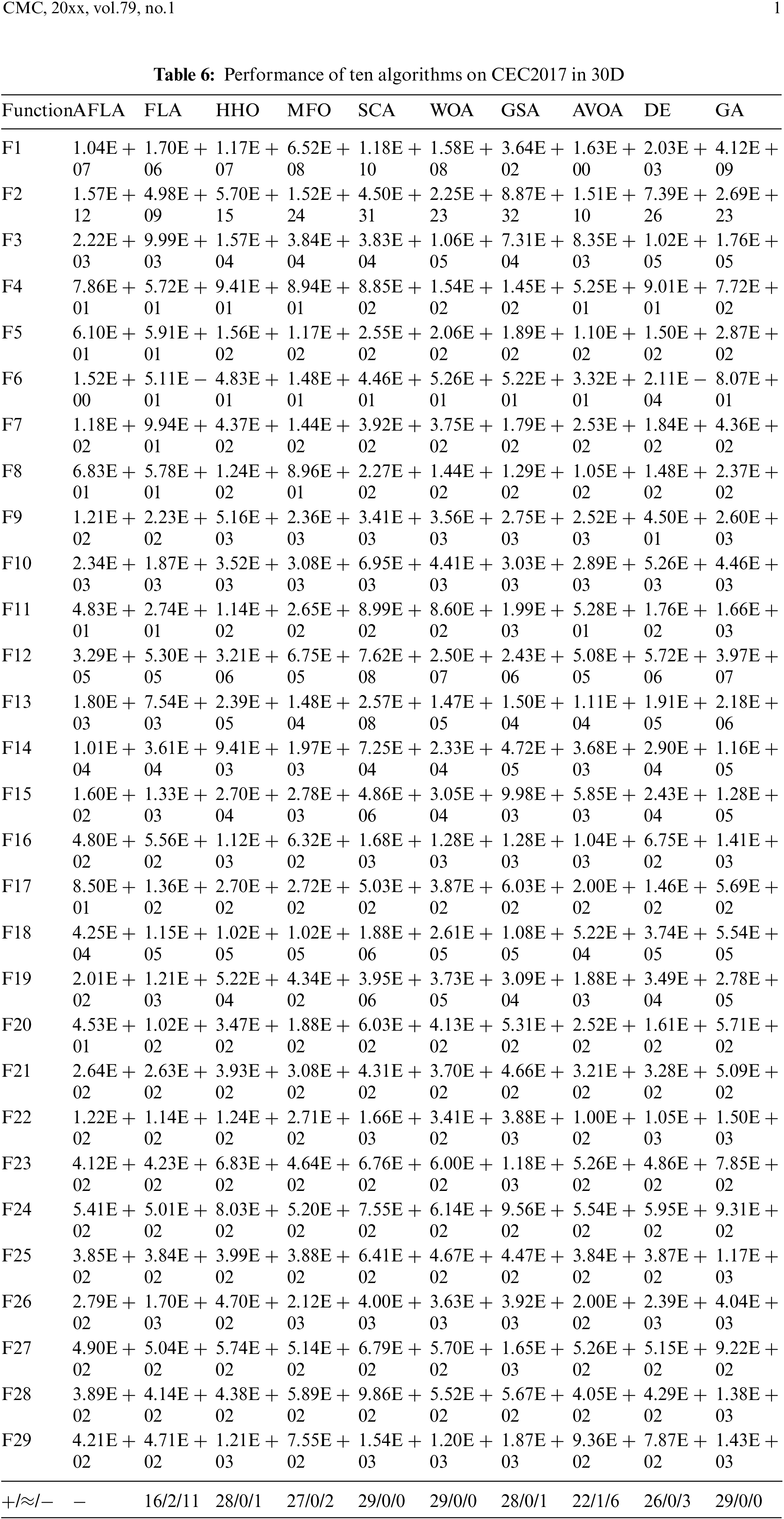
From Table 6, it is evident that AFLA outperforms FLA in 16 functions, surpasses HHO in 28 functions, exceeds MFO in 27 functions, outshines SCA in all 29 functions, surpasses WOA in all 29 functions, performs better than GSA in 28 functions, outperforms AVOA in 22 functions, exceeds DE in 26 functions, and outperforms GA in all 29 functions. Finally, we assert that AFLA demonstrates commendable performance across the 29 functions of CEC2017 in 30D.

5.2.3 Result of 50D

The performance of AFLA and nine comparative algorithms on the 50D benchmark functions of CEC2017 is presented in Table 7.

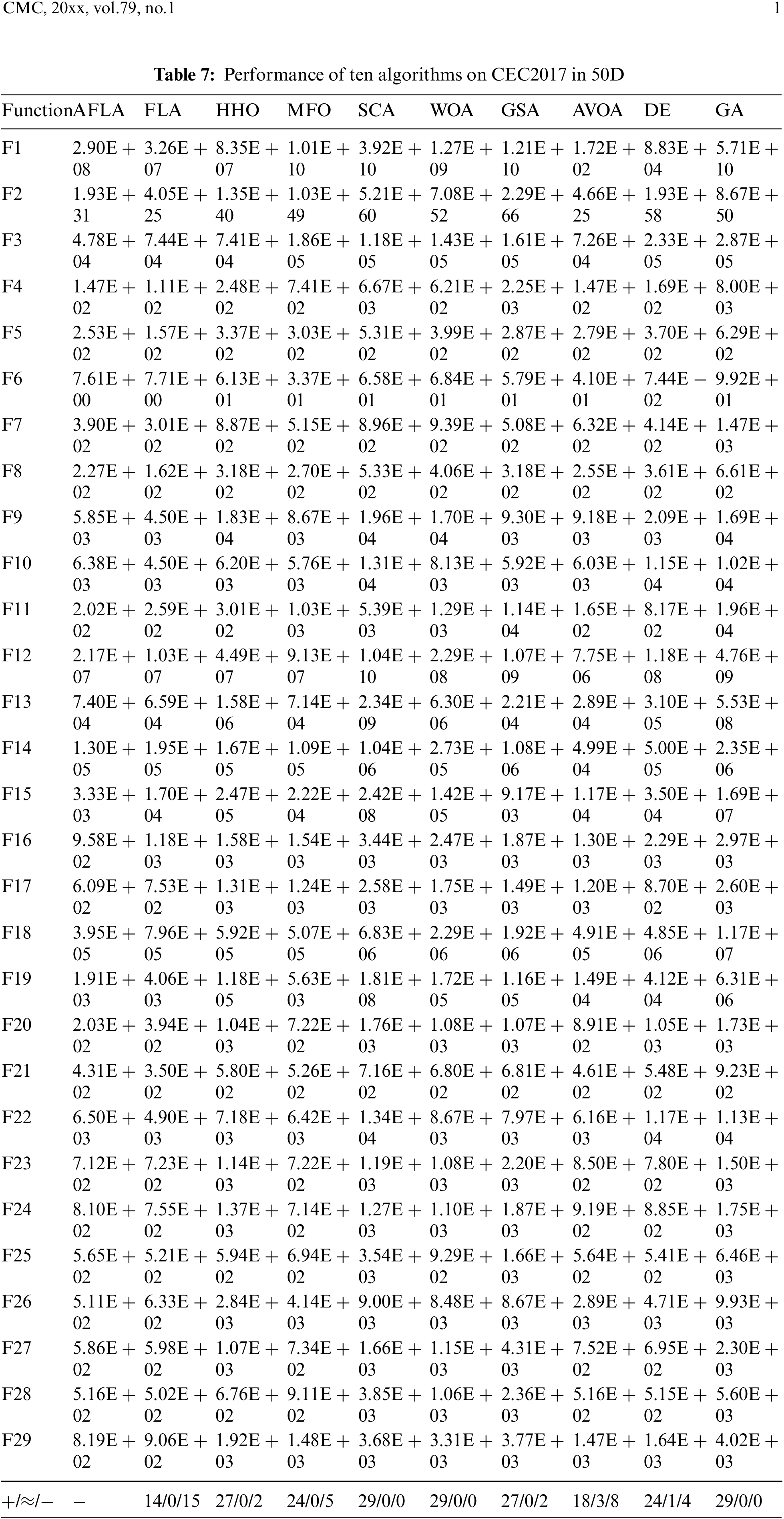
From Table 7, it is evident that AFLA outperforms FLA in 14 functions, surpasses HHO in 27 functions, exceeds MFO in 24 functions, outshines SCA in all 29 functions, surpasses WOA in all 29 functions, performs better than GSA in 27 functions, outperforms AVOA in 18 functions, exceeds DE in 24 functions, and outperforms GA in all 29 functions. In conclusion, we assert that AFLA demonstrates commendable performance across the 29 functions of CEC2017 in 50D.

5.3 Discussion of Experimental Results

In this experiment, we aimed to evaluate the performance of the AFLA algorithm within the CEC2013 and CEC2017 datasets and compare it with other algorithms to validate its effectiveness.

According to the experimental results on CEC2013, AFLA has a significant advantage over the original FLA in 10D, a slight advantage in 30D, and no advantage in 50D. AFLA has a significant advantage over HHO, MFO, SCA, WOA, GSA, DE, and GA in 10D, 30D, and 50D. AFLA has a significant advantage over AVOA in 10D, and 30D and a slight advantage in 50D. Therefore, the proposed AFLA has a significant performance advantage over most of the other algorithms at CEC2013, especially in low dimensions. However, the performance is slightly inferior compared to FLA and AVOA on 50D.

According to the experimental results on CEC2017, AFLA has a significant advantage over the original FLA in 10D, a slight advantage in 30 D, and no advantage in 50D. The proposed AFLA has a significant advantage over HHO, MFO, SCA, WOA, GSA, AVOA, DE, and GA in 10D, 30D, and 50D. Therefore, the proposed AFLA has a significant performance advantage over other algorithms except FLA at CEC2017. However, the performance of AFLA over FLA on 50D is slightly insufficient.

The experimental results indicate that AFLA demonstrates significant advantages in 10D, 30D, and 50D within CEC2013 and CEC2017, particularly excelling in lower dimensions. However, in a few functions or specific dimensions, its performance slightly falls short. For instance, as the dimensionality increases, AFLA’s performance compared to FLA is not as anticipated, potentially due to experimental settings. Additionally, the presence of stochastic elements in the experiment could affect result stability.

6  AFLA-SCNN Model Experimentation in HSI

To enhance the precision of HSI classification, we propose the AFLA-SCNN model. To assess the performance of the AFLA-SCNN model, we will utilize the widely used Indian Pines (IP) hyperspectral image dataset and Pavia University (PU) hyperspectral image dataset for validation.

6.1 Dataset Description

6.1.1 Indian Pines (IP)

The Indian Pines dataset was acquired from the Indian Pines test site in the northwest region of Indiana, USA. It consists of pixels with dimensions of 145 × 145, containing 220 spectral bands, with an approximate spatial resolution of 20 m [51,52]. The RGB representation of this dataset is depicted in Fig. 4.

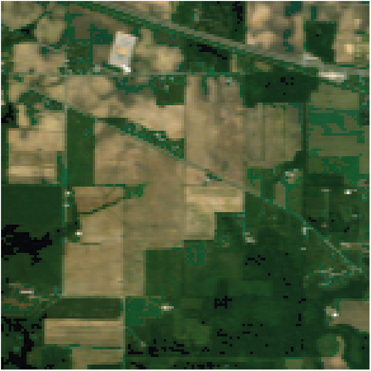
Figure 4: RGB image of Indian Pines

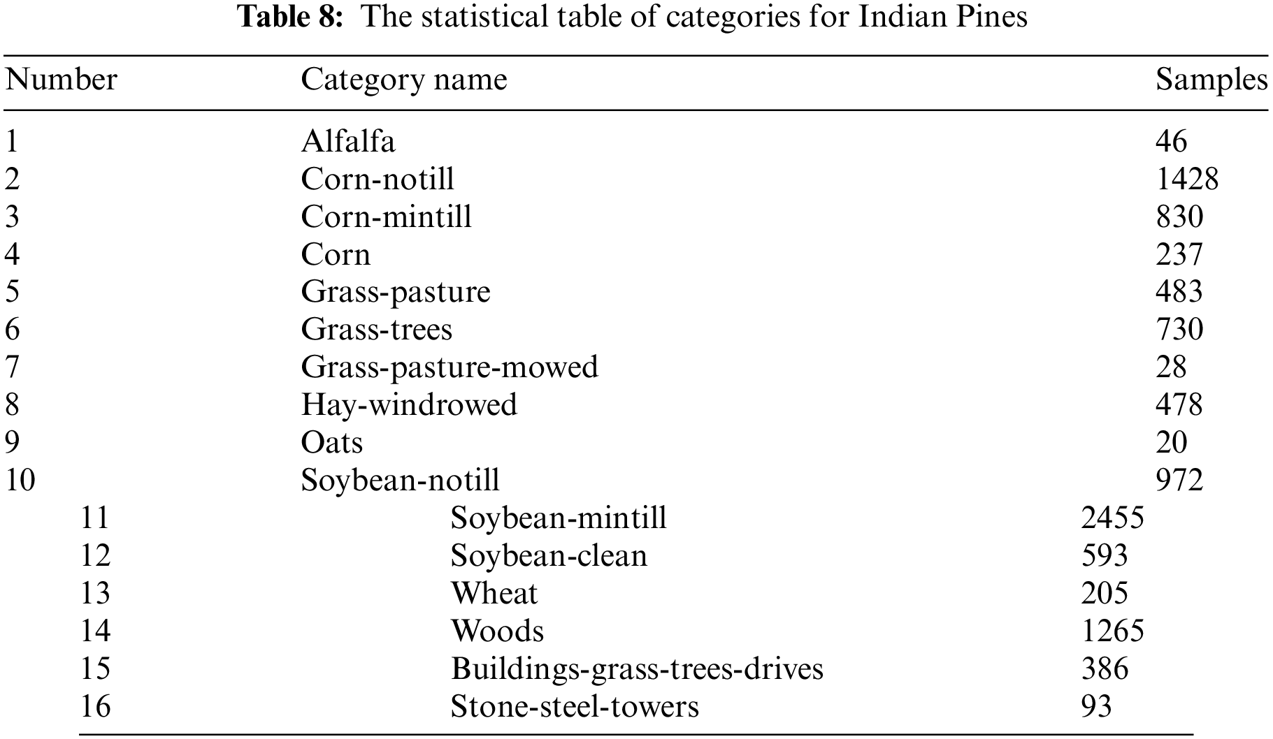
Furthermore, the dataset encompasses 16 categories of vegetation and terrain types such as Alfalfa, Corn, Woods, and more, with specific classification details outlined in Table 8.

6.1.2 Pavia University (PU)

The Pavia University dataset is a hyperspectral data acquired by the Reflectance Optical Spectral Imaging System (ROSIS) over Pavia, Northern Italy [53,54]. The RGB image representation of this data is shown in Fig. 5.

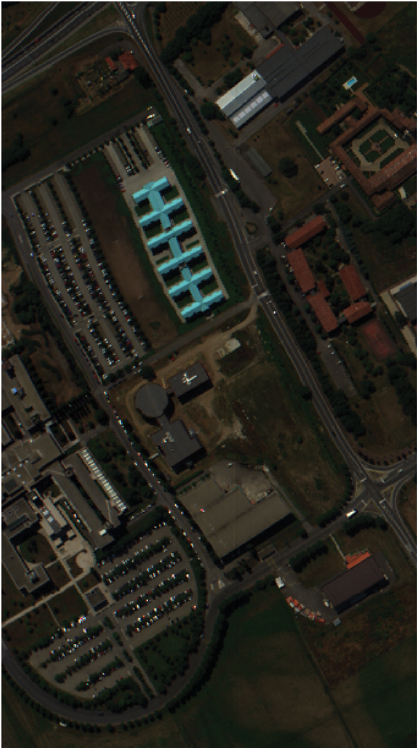
Figure 5: RGB image of Pavia University

6.2 Experimental Design

Firstly, we conducted experimental validation using the AFLA-SCNN model on the IP dataset and the PU dataset. To delve deeper into the performance of this model, we conducted experiments on the same dataset using FLA-SCNN model, HHO-SCNN model, DE-SCNN model, SCNN model, and SVM model. By comparing the experimental outcomes, we aimed to quantitatively assess and validate the superior classification accuracy of the AFLA-SCNN model.

In the AFLA-SCNN model, we set the number of molecules for AFLA to 10 and the maximum iteration count to 50. Since we need to determine the optimal values for the two hyperparameters, “numEpochs” and “miniBatchSize”, we set the dimension to 2. The upper and lower bounds for “numEpochs” are 200 and 1, respectively, while for “miniBatchSize”, the upper and lower bounds are 256 and 32, respectively. Other parameter settings for the AFLA-SCNN model, FLA-SCNN model, HHO-SCNN model, DE-SCNN model, SCNN model, and SVM model are detailed in Table 9.

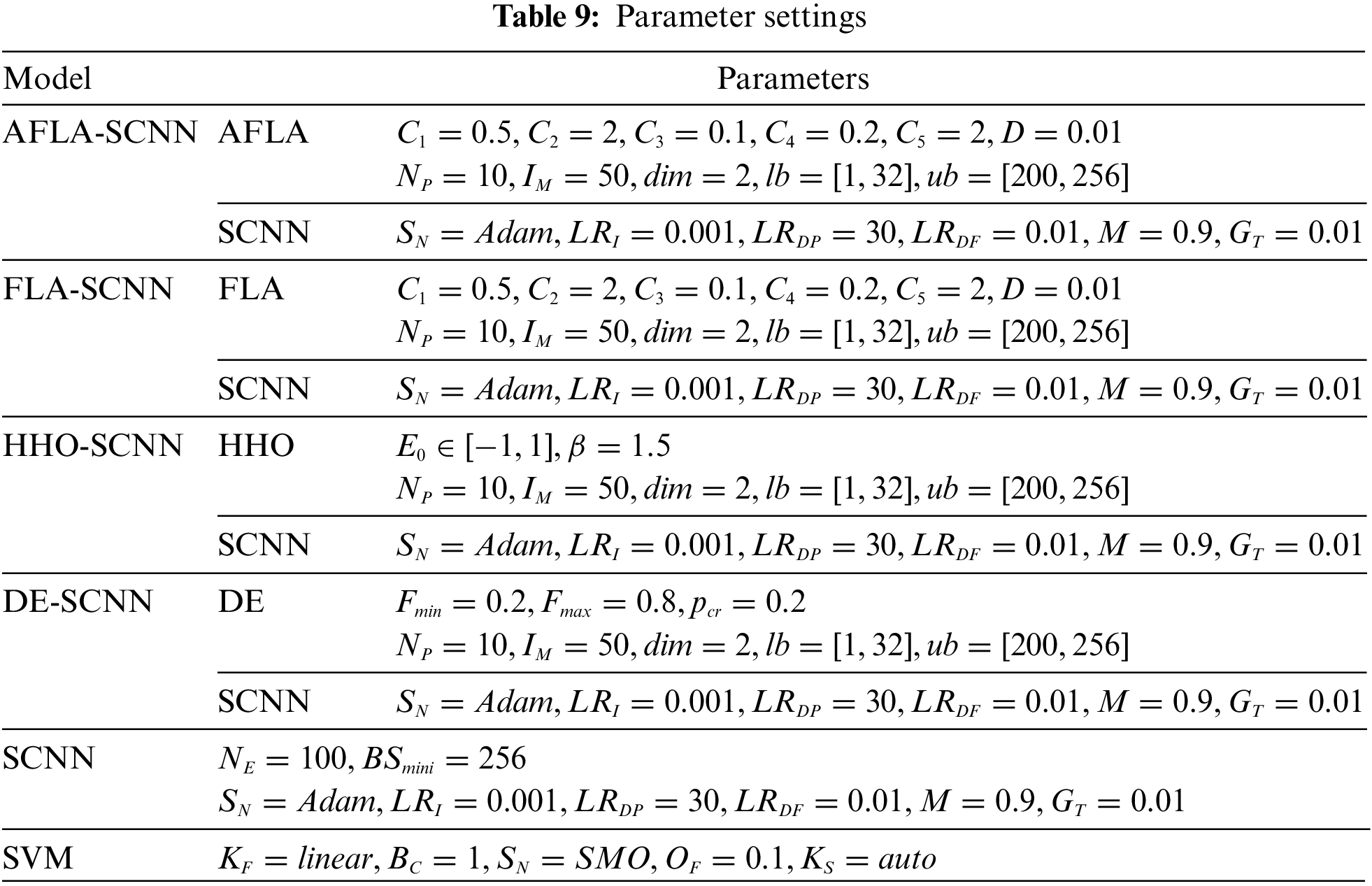
In Table 9, the parameters and settings of different algorithms are clearly listed so that we can compare and analyze them, which are crucial for the performance and results of the algorithm. Firstly, for each algorithm, NP represents the number of particles or populations, that is, the number of individuals simultaneously searching the solution space in the algorithm. IM represents the maximum number of iterations, i.e., the maximum number of rounds the algorithm runs, which determines to what extent the algorithm explores the search space. dim refers to the dimension of the problem, which is the length of the solution vector or the number of features. lb and ub respectively represent the lower and upper bounds of the solution vector, which limit the scope of the search space and ensure the effectiveness of the solution. For SCNN, SN represents the optimizer, which is the algorithm used to update model weights and parameters. LRI is the initial learning rate. LRDP and LRDF respectively represent the number of rounds to reduce the learning rate and the factor to reduce the learning rate. These parameters are used to dynamically adjust the learning rate during the training process to improve convergence speed and stability. M represents the contribution of the gradient step size from the previous iteration to the current iteration. GT is a gradient threshold used to control the size of gradients, which may be used to prevent gradient explosion or disappearance. NE represents the number of training rounds, which is the number of times the entire dataset is used to train the model. BSmini represents the small batch size, which is the number of samples used for each weight update. For SVM, KF represents the kernel function, which determines the calculation method of similarity between data points and is crucial for handling nonlinear problems. BC represents a constraint. SN represents an optimizer. OF represents the expected proportion of outliers in the training data, which helps the algorithm be more robust when dealing with noise or outliers. KS represents the kernel parameter.

All experiments in this paper were conducted using MATLAB R2022b on a system equipped with an Intel(R) Core (TM) i9-11900 processor and 64 GB of RAM running Windows 11.

6.3 Evaluation Metrics

In this section, we delved into the performance metrics used to evaluate the methods proposed in this experiment. The selected indicators aim to comprehensively evaluate the predictive ability of the model while considering its accuracy and reliability. We focus on four key performance indicators: Accuracy, precision, recall, and F1-score.

Accuracy is a fundamental indicator that quantifies the proportion of correctly predicted samples in the total number of samples by the model. It provides a rough overview of model performance, indicating how it performs on the entire dataset. The Accuracy is calculated by dividing the number of correctly predicted samples by the total number of samples, as shown in Eq. (30).

Accuracy=Number of Correctly Classified SamplesTotal Number of Samples(30)

On the other hand, Precision focuses on the quality of model predictions. It represents the proportion of samples that truly belong to a certain category predicted by the model. Precision is crucial in situations where false positives may have significant consequences. It is calculated by dividing the number of true positives (correctly predicted positive samples) by the sum of true positives and false positives (incorrectly predicted positive samples), as shown in Eqs. (31) and (32). Eq. (31) outlines the calculation method for the i-th type Precision, while Eq. (32) provides the average process for all samples.

Precisioni=True PositivesiTotal Predicted as Classi(31)

Precision=∑1nPrecisionin(32)

Recall supplements Precision by examining the model’s ability to recognize all relevant samples. It represents the proportion of samples correctly predicted by the model as belonging to a certain category among all samples that truly belong to that category. Recall is particularly important when missing a positive prediction could have a significant impact. It is calculated by dividing the number of true positives by the sum of true positives and false negatives (incorrectly predicted as negative samples), as shown in Eqs. (33) and (34). Eq. (33) represents the Recall calculation for class i, while Eq. (34) demonstrates the average process of all samples.

Recalli=TruePositivesiActualSamplesasClassi(33)

Recall=∑1nRecallin(34)

Finally, the F1-score is the harmonic mean of Precision and Recall, combining their respective strengths. It aims to comprehensively evaluate the performance of the model, balancing Precision and Recall. The F1-score is calculated by using the bidirectional average of Precision and Recall, as shown in Eqs. (35) and (36). Eq. (35) outlines the F1-score calculation for class i, while Eq. (36) presents the average process for all samples.

F1−scorei=2×Precisioni×RecalliPrecisioni+Recalli(35)

F1−score=∑1nF1−scorein(36)

By using these performance indicators, we aim to comprehensively understand the predictive ability of the proposed method. The results obtained from these calculations will inform us of the strengths and weaknesses of the model, enabling us to make informed decisions regarding its application and potential improvements.

6.4 Experimental Results and Discussion

6.4.1 Experimental Results and Discussion of AFLA-SCNN

After running AFLA-SCNN on the Indian Pines dataset, the obtained optimal values for “numEpochs” and “miniBatchSize” were 155 and 176, respectively. The best fitness value was determined as 9.76E−4 , where its complement number represents the classification accuracy, hence yielding an accuracy rate of 99.90%. However, it is well known that the predictive results of the SCNN model exhibit volatility. Therefore, inputting the optimal values for “numEpochs” and “miniBatchSize” into the SCNN model may not necessarily result in the same accuracy of 99.90%.

After inputting the optimal values for “numEpochs” and “miniBatchSize” obtained from running the AFLA-SCNN model on the Indian Pines dataset into the SCNN model, resulting in an Accuracy of 99.875%, Precision of 99.681%, Recall of 99.723%, and F1-score of 99.686%. In addition, the ground truth classification image and the predicted classification image are illustrated in Fig. 6. In this figure, Fig. 6a represents the ground truth classification image, while Fig. 6b depicts the predicted classification image. Additionally, it is evident that the predicted classification image significantly resembles the ground truth classification image, displaying only minor differences.

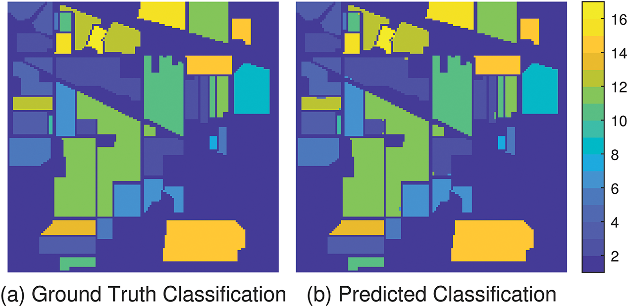
Figure 6: Ground-truth classification images and predicted classification images on IP using AFLA-SCNN model

After running AFLA-SCNN on the Pavia University dataset, the obtained optimal values for “numEpochs” and “miniBatchSize” were 150 and 225, respectively. The best fitness value was determined as 1.65E+0, where its complement number represents the classification accuracy, hence yielding an accuracy rate of 98.35%.

After inputting the optimal values for “numEpochs” and “miniBatchSize” obtained from running the AFLA-SCNN model on the Pavia University dataset into the SCNN model, resulting in an Accuracy of 98.022%, Precision of 92.541 %, Recall of 94.063 %, and F1-score of 93.273 %. In addition, the ground truth classification image and the predicted classification image are illustrated in Fig. 7. In this figure, Fig. 7a represents the ground truth classification image, while Fig. 7b depicts the predicted classification image. Additionally, it is evident that the predicted classification image significantly resembles the ground truth classification image, displaying only minor differences.

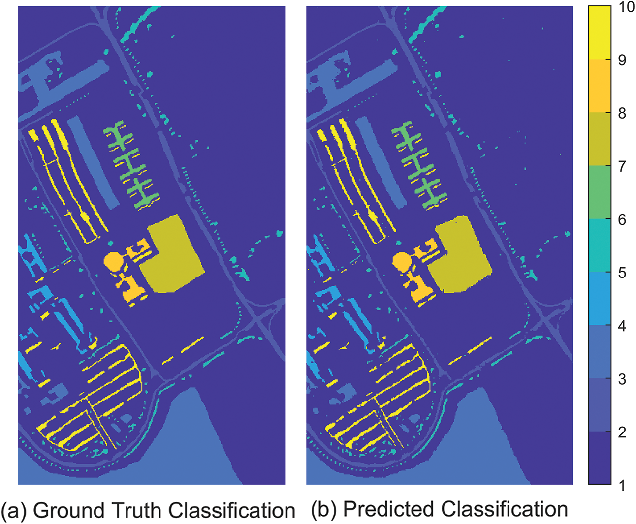
Figure 7: Ground-truth classification images and predicted classification images on PU using AFLA-SCNN model

6.4.2 Experimental Results and Discussion of Comparative Experiment

In this section, we compare the AFLA-SCNN model, FLA-SCNN model, HHO-SCNN model, DE-SCNN model, SCNN model, and SVM model based on evaluation metrics.

Table 10 shows the Accuracy, Precision, Recall, and F1-score of AFLA-SCNN model, FLA-SCNN model, HHO-SCNN model, DE-SCNN model, SCNN model, and SVM model on Indian Pines. Among them, the results of AFLA-SCNN model, FLA-SCNN model, HHO-SCNN model, and DE-SCNN model are obtained by applying the optimized hyperparameters “numEpochs” and “miniBatchSize” obtained by applying the optimized hyperparameters “numEpochs” and “miniBatchSize” to the SCNN model. The optimized hyperparameters “numEpochs” and “miniBatchSize” of FLA-SCNN model on Indian Pines are 199, 256. The values of hyperparameters “numEpochs” and “miniBatchSize” for HHO-SCNN model optimized on Indian Pines are 78, 191. The values of hyperparameters “numEpochs” and “miniBatchSize” for DE-SCNN model optimized on Indian Pines are 54, 189.

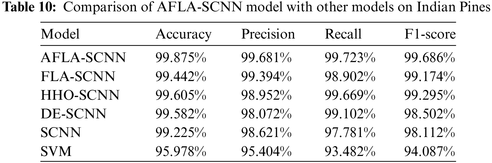
In Table 10, it is evident that the AFLA-SCNN model outperforms the FLA-SCNN model, the HHO-SCNN model, the DE-SCNN model, the SCNN model, and the SVM model in the four evaluation metrics: Accuracy, Precision, Recall, and F1-score. In addition, the AFLA-SCNN model improved 0.65% on Accuracy, 1.06% on Precision, 1.942% on Recall, and 1.574% on F1-score compared to the SCNN model. The AFLA-SCNN model improved 3.897% on Accuracy, 4.277% on Precision, 6.241% on Recall, and 5.599% on F1-score compared to the SVM model. The AFLA-SCNN model improved 0.27% on Accuracy, 0.729% on Precision, 0.054% on Recall, and 0.391% on F1-score compared to the HHO-SCNN model. The AFLA-SCNN model improved 0.293% on Accuracy, 1.609% on Precision, 0.621% on Recall, and 1.184% on F1-score compared to the DE-SCNN model.

However, the AFLA-SCNN model improved 0.433% on Accuracy, 0.287%on Precision, 0.821% on Recall, and 0.512% on F1-score compared to the FLA-SCNN model. The AFLA-SCNN model improves the performance by less than 1% compared to the FLA-SCNN model, so there is still room for improvement of the AFLA-SCNN model in the future.

Table 11 shows the Accuracy, Precision, Recall, and F1-score of AFLA-SCNN model, FLA-SCNN model, HHO-SCNN model, DE-SCNN model, SCNN model, and SVM model on Pavia University. Among them, the results of AFLA-SCNN model, FLA-SCNN model, HHO-SCNN model, and DE-SCNN model are obtained by applying the optimized hyperparameters “numEpochs” and “miniBatchSize” obtained by applying the optimized hyperparameters “numEpochs” and “miniBatchSize” to the SCNN model. The optimized hyperparameters “numEpochs” and “miniBatchSize” of FLA-SCNN model on Pavia University are 126, 243. The values of hyperparameters “numEpochs” and “miniBatchSize” for HHO-SCNN model optimized on Pavia University are 89, 192. The values of hyperparameters “numEpochs” and “miniBatchSize” for DE-SCNN model optimized on Pavia University are 78, 188.

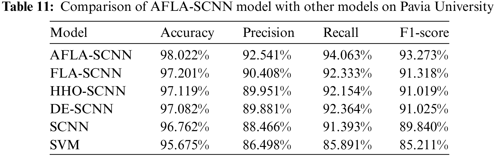
In Table 11, it is evident that the AFLA-SCNN model outperforms the FLA-SCNN model, the HHO-SCNN model, the DE-SCNN model, the SCNN model, and the SVM model in the four evaluation metrics: Accuracy, Precision, Recall, and F1-score. In addition, the AFLA-SCNN model improved 1.26% on Accuracy, 4.075% on Precision, 2.67% on Recall, and 3.433% on F1-score compared to the SCNN model. The AFLA-SCNN model improved 2.347% on Accuracy, 6.043% on Precision, 8.172% on Recall, and 8.062% on F1-score compared to the SVM model. The AFLA-SCNN model improved 0.903% on Accuracy, 2.59% on Precision, 1.909% on Recall, and 2.254% on F1-score compared to the HHO-SCNN model. The AFLA-SCNN model improved 0.94% on Accuracy, 2.66% on Precision, 1.699% on Recall, and 2.248% on F1-score compared to the DE-SCNN model.

However, the AFLA-SCNN model improved 0.821% on Accuracy, 2.133% on Precision, 1.73% on Recall, and 1.955% on F1-score compared to the FLA-SCNN model. The AFLA-SCNN model improves the performance by less than 1% compared to the FLA-SCNN model, so there is still room for improvement of the AFLA-SCNN model in the future.

7  Conclusion

The aim and focal point of this paper are to enhance the accuracy of HSI classification. To achieve this, we propose a Spectral Convolutional Neural Network model based on Adaptive Fick’s Law Algorithm (AFLA-SCNN). This model incorporates our devised Adaptive Fick’s Law Algorithm (AFLA), in which we introduce three novel strategies: Adaptive weight factor, Gaussian mutation, and probability update policy. Subsequently, AFLA is integrated with the SCNN model, leading to the establishment of the AFLA-SCNN model. In this model, we use AFLA to optimize the two hyperparameters “numEpochs” and “miniBatchSize” in the SCNN model to obtain the optimal values of these two parameters and then use the optimal values of these two hyperparameters for HSI classification.

In the experimental part, we first validate the performance of AFLA, and we compare AFLA with 9 well-known intelligent optimization algorithms. And we validate it on 10D, 30D, 50D for 28 functions of CEC2013 and 10D, 30D, 50D for 29 functions of CEC2017, respectively. The experimental results show that AFLA has obvious performance advantages over other optimization algorithms. Subsequently, we conducted comparative experiments between AFLA-SCNN model and FLA-SCNN model, HHO-SCNN model, DE-SCNN model, SCNN model, SVM model on the Indian Pines dataset and Pavia University dataset. The experimental results show that the AFLA-SCNN model outperforms other models in terms of Accuracy, Precision, Recall, and F1-score on Indian Pines and Pavia University. Among them, the Accuracy of the AFLA-SCNN model on Indian Pines reached 99.875%, and the Accuracy on Pavia University reached 98.022%, highlighting the performance of the proposed AFLA-SCNN model in hyperspectral image classification. However, compared with the FLA-SCNN model, the improvement performance of the AFLA-SCNN model is less than 1%, indicating that the model still needs improvement.

In conclusion, the proposed AFLA-SCNN model demonstrates a significant improvement in the accuracy of HSI classification. This presents a novel and effective choice for model selection in analogous domains, offering valuable insights for future relevant research.

Acknowledgement: None.

Funding Statement: This research was partially supported by Natural Science Foundation of Shandong Province, China (Grant No. ZR202111230202).

Author Contributions: The authors confirm contribution to the paper as follows: Study conception and design: T.-Y. Wu, H. Li; data collection: S. Kumari, H. Li; analysis and interpretation of results: C.-M. Chen; draft manuscript preparation: T.-Y. Wu, H. Li, S. Kumari, C.-M. Chen. All authors reviewed the results and approved the final version of the manuscript.

Availability of Data and Materials: The data are contained within the article.

Conflicts of Interest: The authors declare that they have no conflicts of interest to report regarding the present study.

References

1. U. A. Bhatti et al., “MFFCG–Multi feature fusion for hyperspectral image classification using graph attention network,” Expert Syst. Appl., vol. 229, no. 3, pp. 120496, 2023. doi: 10.1016/j.eswa.2023.120496. [Google Scholar] [CrossRef]

2. U. A. Bhatti et al., “Deep learning-based trees disease recognition and classification using hyperspectral data,” Comput., Mater. Contin., vol. 77, no. 1, pp. 681–697, 2023. doi: 10.32604/cmc.2023.037958. [Google Scholar] [CrossRef]

3. S. Li, W. Song, L. Fang, Y. Chen, P. Ghamisi and J. A. Benediktsson, “Deep learning for hyperspectral image classification: An overview,” IEEE Trans. Geosci. Remote Sens., vol. 57, no. 9, pp. 6690–6709, 2019. doi: 10.1109/TGRS.2019.2907932. [Google Scholar] [CrossRef]

4. M. J. Khan, H. S. Khan, A. Yousaf, K. Khurshid, and A. Abbas, “Modern trends in hyperspectral image analysis: A review,” IEEE Access, vol. 6, pp. 14118–14129, 2018. doi: 10.1109/ACCESS.2018.2812999. [Google Scholar] [CrossRef]

5. W. H. Su and D. W. Sun, “Fourier transform infrared and Raman and hyperspectral imaging techniques for quality determinations of powdery foods: A review,” Compr. Rev. Food Sci. Food Saf., vol. 17, no. 1, pp. 104–122, 2018. doi: 10.1111/1541-4337.12314 [Google Scholar] [PubMed] [CrossRef]

6. X. Yang, Y. Ye, X. Li, R. Y. Lau, X. Zhang and X. Huang, “Hyperspectral image classification with deep learning models,” IEEE Trans. Geosci. Remote Sens., vol. 56, no. 9, pp. 5408–5423, 2018. doi: 10.1109/TGRS.2018.2815613. [Google Scholar] [CrossRef]

7. L. Zhang, G. S. Xia, T. Wu, L. Lin, and X. C. Tai, “Deep learning for remote sensing image understanding,” J. Sens., vol. 2016, pp. 7954154, 2016. doi: 10.1155/2016/7954154. [Google Scholar] [CrossRef]

8. L. Mou, P. Ghamisi, and X. X. Zhu, “Deep recurrent neural networks for hyperspectral image classification,” IEEE Trans. Geosci. Remote Sens., vol. 55, no. 7, pp. 3639–3655, 2017. doi: 10.1109/TGRS.2016.2636241. [Google Scholar] [CrossRef]

9. J. Li, J. M. Bioucas-Dias, and A. Plaza, “Spectral-spatial classification of hyperspectral data using loopy belief propagation and active learning,” IEEE Trans. Geosci. Remote Sens., vol. 51, no. 2, pp. 844–856, 2012. doi: 10.1109/TGRS.2012.2205263. [Google Scholar] [CrossRef]

10. O. Okwuashi and C. E. Ndehedehe, “Deep support vector machine for hyperspectral image classification,” Pattern Recogn., vol. 103, no. 4, pp. 107298, 2020. doi: 10.1016/j.patcog.2020.107298. [Google Scholar] [CrossRef]

11. A. L. H. P. Shaik, M. K. Manoharan, A. K. Pani, R. R. Avala, and C. M. Chen, “Gaussian mutation-spider monkey optimization (GM-SMO) model for remote sensing scene classification,” Remote Sens., vol. 14, no. 24, pp. 6279, 2022. doi: 10.3390/rs14246279. [Google Scholar] [CrossRef]

12. D. Hong, L. Gao, J. Yao, B. Zhang, A. Plaza and J. Chanussot, “Graph convolutional networks for hyperspectral image classification,” IEEE Trans. Geosci. Remote Sens., vol. 59, no. 7, pp. 5966–5978, 2020. doi: 10.1109/TGRS.2020.3015157. [Google Scholar] [CrossRef]

13. S. Ghaderizadeh, D. Abbasi-Moghadam, A. Sharifi, N. Zhao, and A. Tariq, “Hyperspectral image classification using a hybrid 3D-2D convolutional neural networks,” IEEE J. Select. Top. Appl. Earth Observ. Remote Sens., vol. 14, pp. 7570–7588, 2021. doi: 10.1109/JSTARS.2021.3099118. [Google Scholar] [CrossRef]

14. S. Jia, S. Jiang, S. Zhang, M. Xu, and X. Jia, “Graph-in-graph convolutional network for hyperspectral image classification,” IEEE Trans. Neural Netw. Learn. Syst., vol. 35, no. 1, pp. 1157–1171, Jan. 2024. doi: 10.1109/TNNLS.2022.3182715 [Google Scholar] [PubMed] [CrossRef]

15. H. Ge et al., “Two-branch convolutional neural network with polarized full attention for hyperspectral image classification,” Remote Sens., vol. 15, no. 3, pp. 848, 2023. doi: 10.3390/rs15030848. [Google Scholar] [CrossRef]

16. T. Y. Wu, H. Li, and S. C. Chu, “CPPE: An improved phasmatodea population evolution algorithm with chaotic maps,” Math., vol. 11, no. 9, pp. 1977, 2023. doi: 10.3390/math11091977. [Google Scholar] [CrossRef]

17. X. K. Liu, P. Q. Li, Z. K. Zhang, and J. Zen, “Location and capacity determination of energy storage system based on improved whale optimization algorithm,” J. Netw. Intell., vol. 8, pp. 35–46, 2023. [Google Scholar]

18. J. S. Pan, L. Li, S. C. Chu, K. K. Tseng, and H. A. Shehadeh, “Martial art learning optimization: A novel metaheuristic algorithm for night image enhancement,” J. Internet Technol., vol. 24, no. 7, pp. 1415–1428, 2023. doi: 10.53106/160792642023122407003. [Google Scholar] [CrossRef]

19. T. Y. Wu, A. Shao, and J. S. Pan, “CTOA: Toward a chaotic-based tumbleweed optimization algorithm,” Math., vol. 11, no. 10, pp. 2339, 2023. doi: 10.3390/math11102339. [Google Scholar] [CrossRef]

20. C. M. Chen, S. Lv, J. Ning, and J. M. T. Wu, “A genetic algorithm for the waitable time-varying multi-depot green vehicle routing problem,” Symmetry, vol. 15, no. 1, pp. 124, 2023. doi: 10.3390/sym15010124. [Google Scholar] [CrossRef]

21. F. B. Banadkooki et al., “Suspended sediment load prediction using artificial neural network and ant lion optimization algorithm,” Environ. Sci. Pollut. Res., vol. 27, no. 30, pp. 38094–38116, 2020. doi: 10.1007/s11356-020-09876-w [Google Scholar] [PubMed] [CrossRef]

22. S. Nikbakht, C. Anitescu, and T. Rabczuk, “Optimizing the neural network hyperparameters utilizing genetic algorithm,” J. Zhejiang Univ.-Sci. A, vol. 22, no. 6, pp. 407–426, 2021. doi: 10.1631/jzus.A2000384. [Google Scholar] [CrossRef]

23. Y. Fan, Y. Zhang, B. Guo, X. Luo, Q. Peng and Z. Jin, “A hybrid sparrow search algorithm of the hyperparameter optimization in deep learning,” Math., vol. 10, no. 16, pp. 3019, 2022. doi: 10.3390/math10163019. [Google Scholar] [CrossRef]

24. M. R. Falahzadeh, F. Farokhi, A. Harimi, and R. Sabbaghi-Nadooshan, “Deep convolutional neural network and gray wolf optimization algorithm for speech emotion recognition,” Circ., Syst. Signal Process., vol. 42, no. 1, pp. 449–492, 2023. doi: 10.1007/s00034-022-02130-3. [Google Scholar] [CrossRef]

25. F. A. Hashim, R. R. Mostafa, A. G. Hussien, S. Mirjalili, and K. M. Sallam, “Fick’s law algorithm: A physical law-based algorithm for numerical optimization,” Knowl.-Based Syst., vol. 260, no. 2, pp. 110146, 2023. doi: 10.1016/j.knosys.2022.110146. [Google Scholar] [CrossRef]

26. A. S. Alghamdi et al., “Energy hub optimal scheduling and management in the day-ahead market considering renewable energy sources, CHP, electric vehicles, and storage systems using improved Fick’s law algorithm,” Appl. Sci., vol. 13, no. 6, pp. 3526, 2023. doi: 10.3390/app13063526. [Google Scholar] [CrossRef]

27. P. Mehta, B. S. Yildiz, S. M. Sait, and A. R. Yildiz, “A novel hybrid Fick’s law algorithm-quasi oppositional-based learning algorithm for solving constrained mechanical design problems,” Mater. Test., vol. 65, pp. 1817–1825, 2023. doi: 10.1515/mt-2023-0235. [Google Scholar] [CrossRef]

28. H. Li, S. C. Chu, S. Kumari, and T. Y. Wu, “Fick’s law algorithm with Gaussian mutation: Design and analysis,” in Int. Conf. Gene. Evol. Comput., Kaohsiung, Taiwan, Springer, 2023, pp. 456–467. [Google Scholar]

29. X. Zhang et al., “Understanding the learning mechanism of convolutional neural networks in spectral analysis,” Anal. Chim. Acta, vol. 1119, pp. 41–51, 2020. doi: 10.1016/j.aca.2020.03.055 [Google Scholar] [PubMed] [CrossRef]

30. S. Mei, R. Jiang, X. Li, and Q. Du, “Spatial and spectral joint super-resolution using convolutional neural network,” IEEE Trans. Geosci. Remote Sens., vol. 58, no. 7, pp. 4590–4603, 2020. doi: 10.1109/TGRS.2020.2964288. [Google Scholar] [CrossRef]

31. B. Lu, P. D. Dao, J. Liu, Y. He, and J. Shang, “Recent advances of hyperspectral imaging technology and applications in agriculture,” Remote Sens., vol. 12, no. 16, pp. 2659, 2020. doi: 10.3390/rs12162659. [Google Scholar] [CrossRef]

32. S. A. Shevchik, C. Kenel, C. Leinenbach, and K. Wasmer, “Acoustic emission for in situ quality monitoring in additive manufacturing using spectral convolutional neural networks,” Addit. Manufact., vol. 21, no. Suppl. 1, pp. 598–604, 2018. doi: 10.1016/j.addma.2017.11.012. [Google Scholar] [CrossRef]

33. A. Zhang, H. Xu, W. Bi, and S. Xu, “Adaptive mutant particle swarm optimization based precise cargo airdrop of unmanned aerial vehicles,” Appl. Soft Comput., vol. 130, no. 99, pp. 109657, 2022. doi: 10.1016/j.asoc.2022.109657. [Google Scholar] [CrossRef]

34. S. Song et al., “Dimension decided Harris hawks optimization with Gaussian mutation: Balance analysis and diversity patterns,” Knowl.-Based Syst., vol. 215, no. 5, pp. 106425, 2021. doi: 10.1016/j.knosys.2020.106425. [Google Scholar] [CrossRef]

35. S. Liu et al., “Human memory update strategy: A multi-layer template update mechanism for remote visual monitoring,” IEEE Trans. Multimed., vol. 23, pp. 2188–2198, 2021. doi: 10.1109/TMM.2021.3065580. [Google Scholar] [CrossRef]

36. E. Kristiani, C. F. Lee, C. T. Yang, C. Y. Huang, Y. T. Tsan and W. C. Chan, “Air quality monitoring and analysis with dynamic training using deep learning,” J. Supercomput., vol. 77, no. 6, pp. 5586–5605, 2021. doi: 10.1007/s11227-020-03492-8. [Google Scholar] [CrossRef]

37. S. Lee et al., “Improving scalability of parallel CNN training by adjusting mini-batch size at run-time,” in 2019 IEEE Int. Conf. Big Data (Big Data), Long Beach, CA, USA, IEEE, 2019, pp. 830–839. [Google Scholar]

38. N. Gazagnadou, R. Gower, and J. Salmon, “Optimal mini-batch and step sizes for saga,” in Int. Conf. Mach. Learn., Los Angeles, CA, USA, PMLR, 2019, pp. 2142–2150. [Google Scholar]

39. M. S. Maučec and J. Brest, “A review of the recent use of differential evolution for large-scale global optimization: An analysis of selected algorithms on the CEC 2013 LSGO benchmark suite,” Swarm Evol. Comput., vol. 50, pp. 100428, 2019. [Google Scholar]

40. J. O. Agushaka, O. Akinola, A. E. Ezugwu, O. N. Oyelade, and A. K. Saha, “Advanced dwarf mongoose optimization for solving CEC, 2011 and CEC, 2017 benchmark problems,” PLoS One, vol. 17, no. 11, pp. e0275346, 2022. doi: 10.1371/journal.pone.0275346 [Google Scholar] [PubMed] [CrossRef]

41. A. A. Heidari, S. Mirjalili, H. Faris, I. Aljarah, M. Mafarja and H. Chen, “Harris hawks optimization: Algorithm and applications,” Future Gener. Comput. Syst., vol. 97, pp. 849–872, 2019. doi: 10.1016/j.future.2019.02.028. [Google Scholar] [CrossRef]

42. S. Mirjalili, “Moth-flame optimization algorithm: A novel nature-inspired heuristic paradigm,” Knowl.-Based Syst., vol. 89, pp. 228–249, 2015. doi: 10.1016/j.knosys.2015.07.006. [Google Scholar] [CrossRef]

43. S. Mirjalili, “SCA: A sine cosine algorithm for solving optimization problems,” Knowl.-Based Syst., vol. 96, no. 63, pp. 120–133, 2016. doi: 10.1016/j.knosys.2015.12.022. [Google Scholar] [CrossRef]

44. S. Mirjalili and A. Lewis, “The whale optimization algorithm,” Adv. Eng. Softw., vol. 95, no. 12, pp. 51–67, 2016. doi: 10.1016/j.advengsoft.2016.01.008. [Google Scholar] [CrossRef]

45. E. Rashedi, H. Nezamabadi-Pour, and S. Saryazdi, “GSA: A gravitational search algorithm,” Inform. Sci., vol. 179, no. 13, pp. 2232–2248, 2009. doi: 10.1016/j.ins.2009.03.004. [Google Scholar] [CrossRef]

46. B. Abdollahzadeh, F. S. Gharehchopogh, and S. Mirjalili, “African vultures optimization algorithm: A new nature-inspired metaheuristic algorithm for global optimization problems,” Comput. Ind. Eng., vol. 158, no. 4, pp. 107408, 2021. doi: 10.1016/j.cie.2021.107408. [Google Scholar] [CrossRef]

47. K. V. Price, “Differential evolution,” in Handbook of Optimization: From Classical to Modern Approach. Berlin, Heidelberg: Springer, 2013, pp. 187–214. [Google Scholar]

48. S. Mirjalili and S. Mirjalili, “Genetic algorithm,” Evol. Algo. Neural Netw.: Theory Appl., vol. 780, pp. 43–55, 2019. doi: 10.1007/978-3-319-93025-1. [Google Scholar] [CrossRef]

49. J. J. Liang, B. Qu, P. N. Suganthan, and A. G. Hernández-Díaz, “Problem definitions and evaluation criteria for the CEC 2013 special session on real-parameter optimization,” Technic. Report, Computational Intelligence Laboratory, Zhengzhou University, Zhengzhou, China and Nanyang Technological University, Singapore, vol. 201212, no. 34, pp. 281–295, 2013. [Google Scholar]

50. G. Wu, R. Mallipeddi, and P. N. Suganthan, “Problem definitions and evaluation criteria for the CEC 2017 competition on constrained real-parameter optimization,” Technic. Report, National University of Defense Technology, Changsha, Hunan, China and Kyungpook National University, Daegu, South Korea and Nanyang Technological University, Singapore, 2017. [Google Scholar]

51. A. Zare and P. Gader, “Hyperspectral band selection and endmember detection using sparsity promoting priors,” IEEE Geosci. Remote Sens. Lett., vol. 5, no. 2, pp. 256–260, 2008. doi: 10.1109/LGRS.2008.915934. [Google Scholar] [CrossRef]

52. P. Ghamisi and J. A. Benediktsson, “Feature selection based on hybridization of genetic algorithm and particle swarm optimization,” IEEE Geosci. Remote Sens. Lett., vol. 12, no. 2, pp. 309–313, 2014. doi: 10.1109/LGRS.2014.2337320. [Google Scholar] [CrossRef]

53. M. E. Paoletti, J. M. Haut, J. Plaza, and A. Plaza, “A new deep convolutional neural network for fast hyperspectral image classification,” ISPRS J. Photogramm. Remote Sens., vol. 145, no. 4, pp. 120–147, 2018. doi: 10.1016/j.isprsjprs.2017.11.021. [Google Scholar] [CrossRef]

54. P. Ghamisi, R. Souza, J. A. Benediktsson, L. Rittner, R. Lotufo and X. X. Zhu, “Hyperspectral data classification using extended extinction profiles,” IEEE Geosci. Remote Sens. Lett., vol. 13, no. 11, pp. 1641–1645, 2016. doi: 10.1109/LGRS.2016.2600244. [Google Scholar] [CrossRef]