Research on Driver’s Fatigue Detection Based on Information Fusion

1  Introduction

Fatigue driving refers to the decline of drivers’ physiological function due to long-term continuous driving or lack of sleep, which affects drivers’ regular driving operation [1]. The behavior is mainly manifested by prolonged eye closure, yawning, and frequent nodding, and the physiological performance is primarily indicated by slow heartbeat and slow breathing. These characteristics can be used to identify the fatigue driving behavior and warn drivers to avoid potential traffic accidents. Therefore, it is of great significance to study the driver fatigue recognition algorithm. In all significant traffic accidents, 27% of drivers are tired. In railway traffic, the proportion of train accidents caused by train driver fatigue is as high as 30%~40% [2]. Although napping while driving is a severe violation of discipline, drivers still frequently experience fatigue due to various factors such as nighttime driving, long driving hours, and short rest periods [3]. Many accidents are directly or indirectly related to drivers’ states. Toyota investigated the causes of traffic accidents [4], as shown in Fig. 1. 92.9% of traffic accidents are directly or indirectly caused by humans, among the three factors. The driver’s driving state will directly affect the operation error rate and the ability to deal with emergencies. Driving fatigue has become an invisible killer of traffic accidents [5].

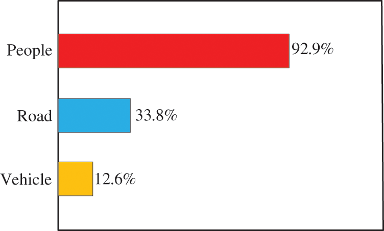
Figure 1: Statistics of accident factors

The prevention of driver fatigue is the focus of the road traffic safety field, and the recognition of driver fatigue is the prerequisite for preventing driver fatigue. Driver fatigue recognition methods have been extensively developed, and several driver fatigue recognition techniques (lane departure, image recognition) have been applied to certain vehicles [6].

(1) Driver fatigue detection based on facial features evaluates fatigue according to facial expression when the driver enters the fatigue state [7]. As a non-contact detection method, this method does not affect driving. However, objective factors such as light and occlusion (glasses and hair) easily affect image information collected in the driving environment. Balasundaram et al. developed a method to extract specific features of eyes to determine the degree of drowsiness but did not consider the influence of blinking and other factors on fatigue driving [8]. Garg recognized a driver’s sleepiness while measuring parameters such as blinking frequency, eye closure, and yawning [9]. Wang et al. monitored drivers’ eye movement data and behavior and selected indicators such as the proportion of eye closing time through experiments [10]. Ye et al. proposed a driver fatigue detection system based on residual channel attention network and head pose estimation. This system used a Retina face for face location; five face landmarks were output [11].

(2) Physiological information can most truly reflect the fatigue state of drivers, and the amount of data of physiological signals is much smaller than that of image information [12]. However, the disadvantage is that collecting various physiological information is invasive to the human body. Physiological signals commonly used to detect driver fatigue include EEG, electrocardiogram (EOG), electromyography (EMG), respiration, pulse, etc. When the driver is tired, the driver’s physiological parameters and non-fatigue state have different changes. Based on the detection model established by Thilagaraj, the EEG signals were classified, and fatigue detection was realized [13]. Lv et al. preprocessed the EEG signal, selected feature value, and used a clustering algorithm to classify the driver fatigue and label the EEG feature data set according to driving quality [14]. Watling et al. conducted a comprehensive and systematic review of recent techniques for detecting driver sleepiness using physiological signals [15]. Murugan et al. detected and analyzed the drivers’ state by monitoring the electrocardiogram signal [16]. Priyadharshini et al. calculated the blood oxygen level in the driver’s blood to determine and assess the driver’s sleepiness [17]. Sun et al. studied changes in blood oxygen saturation under mental fatigue [18]. During the experiment, blood oxygen saturation of brain tissue was monitored in real-time using near-infrared spectroscopy. Results showed that mental fatigue and reaction speed decreased after participating in the task, and the blood oxygen saturation of brain tissue increased compared with non-participating tasks. It can be concluded that mental fatigue affected performance, and brain tissue’s blood oxygen saturation level was also more affected by a test’s motivation and compensation mechanism than by resting level.

(3) Fatigue driving detection based on vehicle driving characteristics indirectly predicts fatigue state by measuring the vehicle’s driving speed, curve size, and angle of deviation from the driving line [19]. After entering a fatigued state, the driving ability will be significantly reduced, and attention will be low, which will cause the vehicle to deviate from the driving line. The advantage of this method is that it can ensure the safety of drivers to the maximum extent. Still, the disadvantages are low accuracy and poor night driving detection, so it is rarely used. Mercedes-Benz’s Attention Assist extracted speed, acceleration, angle, and other information about the vehicle, and it conducted comprehensive processing to detect fatigue state [20].

However, due to the complex mechanism of fatigue, numerous influencing factors, and significant differences in individual performance, there are still many difficulties in the practical application of driver fatigue recognition, so the current key road traffic industry still needs to adjust or control the driving time to avoid fatigue driving. In addition, a single feature’s high false detection rate generally can not accurately detect the fatigue state, and fatigue behavior is related to facial image features and other physiological parameters. To improve the accuracy and stability of fatigue driving detection, this paper focused on fatigue feature extraction and information fusion, designed a comprehensive simulation driving experiment, established a fatigue driving sample dataset, and verified the detection effect. The research content is as follows: The Sections 1 introduces the research status of fatigue driving. In Sections 2, methods of fatigue feature extraction based on drivers’ facial images and biological signals are introduced. Sections 3 fuses heterogeneous information of image information and physiological signals in fatigue scenarios to improve the accuracy and robustness of fatigue detection. In Sections 4, the construction of a comprehensive simulation driving experiment platform, design of the experimental process, and data collection are introduced, and the effect of various fatigue analysis algorithms is verified by data collected during experiments. Sections 5 concludes the paper and puts forward prospects.

2  Research on Fatigue Feature Extraction Method

When entering a fatigued state, drivers have different physiological function declines [21], which can be judged by analyzing drivers’ facial images and biological signals. This section introduces the extraction of feature parameters related to fatigue from the collected and physical signals.

2.1 Fatigue Feature Extraction Based on Image Information

Driver fatigue detection based on image information is the most applied method. When entering the fatigue state, drivers’ eye features will have apparent changes, which can be used to evaluate the fatigue state.

2.1.1 Driver Face Detection Algorithm Based on Histogram of Oriented Gradients (HOG)

For a fatigue detection system built by machine vision, the image of the driver’s face must be obtained first. Subsequent facial vital points and driver fatigue features can be extracted. Therefore, applying a fast and accurate face detection algorithm for a fatigue detection system is essential.

Compared with other image detection algorithms, HOG quantifies the gradient direction of the image in a cellular manner to characterize the structural features of object edges [22]. As the algorithm quantizes position and orientation space, it reduces the influence of object rotation and translation. Moreover, the gradient information of the object is not easily affected by actual ambient light, and the algorithm consumes fewer computer resources, so it is more suitable to be applied to a driver fatigue detection system with significant light variations and small computational power. The specific face detection process based on the HOG algorithm is as follows:

(1) Image normalization

Since camera input images are mostly RGB color space with high feature dimensions, which is not conducive to direct processing, they must be converted to grayscale images as in Eq. (1). The image compression process was then normalized using the Gamma algorithm to reduce the effects of light, color, and shadows in the actual driving environment scene, as shown in Eq. (2), where (x, y) denotes pixels in the image.

Gray=0.299R+0.587G+0.114B(1)

I(x,y)=I(x,y)gamma(2)

(2) Image pixel gradient calculation

Due to considerable gradient variation at the object shape’s edges, contour information value G (x, y) can be obtained by traversing computed pixel steps. Eqs. (3) and (4) are formulas for calculating gradients in horizontal and vertical directions.

Gx(x,y)=H(x+1,y)−H(x−1,y)(3)

Gy(x,y)=H(x,y+1)−H(x,y−1)(4)

where H(x,y) is the pixel value of the image. After obtaining Gx(x,y) and Gy(x,y) of pixel points through traversal calculation, the gradient value G(x,y) and gradient direction α(x,y) of pixel points were calculated using Eqs. (5) and (6).

G(x,y)=Gx(x,y)2+Gy(x,y)2(5)

α(x,y)=tan−1⁡(Gy(x,y)Gx(x,y))(6)

(3) Gradient histogram construction

The input image was evenly divided into several small regions of the same size, also called cell units, and pixels of each area were n×n. Then, the gradient histogram of each cell was counted.

(4) Merging and normalization of gradient histogram

Aiming at the problem of sizeable front-background light contrast in the driving environment, multiple cells were combined into interoperable unit blocks to reduce gradient intensity change, and then gradient information in each block was normalized to improve algorithm performance. Finally, the unit block was used as a sliding window to scan cockpit image input by the camera, extract HOG features, and input them to the classifier. Non-maximum suppression algorithm [23] was used to process multiple face candidate frames in the output, and face candidate boxes were finally obtained, as shown in Fig. 2.

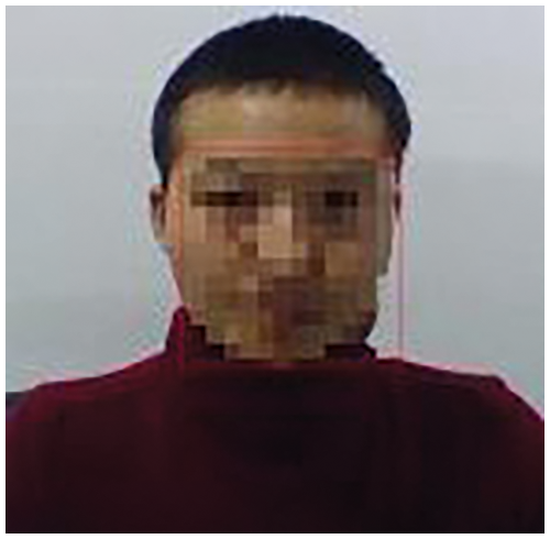
Figure 2: Schematic diagram of driver face position detection

The driver’s position was relatively fixed in the actual driving environment, and the face was in the middle of the collected images. HOG algorithm will not frequently lose detection target due to changes in the driver’s facial expression and driving posture. Therefore, the face detection algorithm based on HOG features has excellent accuracy. Furthermore, since the HOG algorithm’s main principle was to calculate the gradient of the image, most of which were linear operations, low time complexity, and good real-time detection, it is more suitable for onboard systems with small CPU computing capacity.

2.1.2 Eye Feature Points

Face key point detection describes the facial geometric features of face images in machine vision. Given an image with face information, a face key point detection algorithm can identify and locate facial geometric features such as a face’s eyes, mouth, and nose according to target requirements. In this section, based on the image with face and distance information output from the HOG face detection algorithm, the cascade regression tree algorithm was used to locate the driver’s face’s critical point information, laying the foundation for the subsequent fatigue feature extraction.

Eye feature point localization belongs to the category of face alignment, referring to finding various facial landmarks from detected faces, such as eyes, eyebrows, nose, mouth, face outline, and other key positions. The data set used in this paper is 300 W, the number of feature points is 68 points, and there are more than 3000 samples, which meets the requirements of the fatigue driving detection scenario. Table 1 lists the posture information of the dataset.

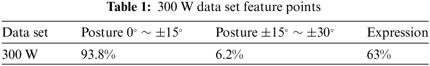
The Ensemble of Regression Trees (ERT) algorithm used in this paper is a face alignment algorithm based on regression trees [24]. By constructing a cascade of Gradient Boost Decision Tree (GBDT) [25], the algorithm made face gradually return from the initial value of feature points to the actual position. The algorithm was implemented in machine learning toolkit Dlib [26]. ERT was used to align the detected face area to find the location of the face, and the detection effect is shown in Fig. 3. Compared with traditional algorithms, ERT can solve the problems of missing or uncertain labels in the training process and minimize the same loss function while performing shape-invariant feature selection. The following introduces eye movement feature extraction based on eye feature points.

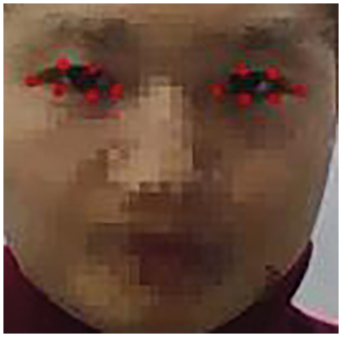
Figure 3: Schematic diagram of eye feature point detection

(1) Reference Fatigue Index

The interval between the driver’s opening and closing eyes in unit time can reveal a fatigue state. PERCLOS defined the proportion of eye closing frame duration in unit time to total detection frame duration. Among them, PERCLOS took the ratio of eye-face closed area to the total eye area as the reference standard, and the ratio reached 50%, 70%, and 80% representing EM, P70, and P80, respectively.

(2) Eyelid Ratio (ER)

ER, which described the ratio of the eye’s height to the eye’s width, was introduced to analyze blinking movements. When people opened their eyes, ER was a relatively stable value, and the corresponding ratio changed when their eyes were closed. As shown in Fig. 4, each eye was calibrated by six-coordinate points P1–P6, taking the right eye as an example.

EAR=|P2−P6|+|P3−P5|2|P1−P4|(7)

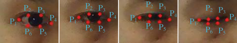
Figure 4: Four typical degrees of eyelid closure

The numerator represented the longitudinal Euclidean distance between points, and the denominator calculated the transverse Euclidean distance between points. Longitudinal points were weighted to ensure coordinates with different distances apply different ratio factors, and the computed ER values have the same scale.

2.2 Fatigue Characteristics Based on Biological Signals

In recent years, many studies have investigated the correlation between cognitive learning tasks, driving fatigue, and other aspects of biological signals [15]. However, the measurement of fatigued driving status has not been standardized, and further research is needed. Relevant studies in the fields of cognitive science and neuroscience have shown that changes in fatigue state are closely related to physiological information, especially to the corresponding activity of the human cerebral cortex and blood oxygen saturation level, laying a theoretical foundation for analysis and recognition of human fatigue state based on cerebral cortex activities and blood oxygen. Physiological electrical signal analysis is the most objective and effective way to monitor human fatigue. Physiological signal features are described as follows.

2.2.1 Noise Reduction of EEG Signals

EEG signals acquired in the driving environment carry multiple interfering signals, including non-physiological and physiological artifacts [27]. It is necessary to investigate the filtering method of EEG artifact components to facilitate subsequent processing. Ocular electrical artifacts caused by human blink and eye movement are the most common physiological artifacts in EEG signals. Typical visual artifact waveforms are shown in Fig. 5, and the labeled red parts are characteristic ocular disturbances.

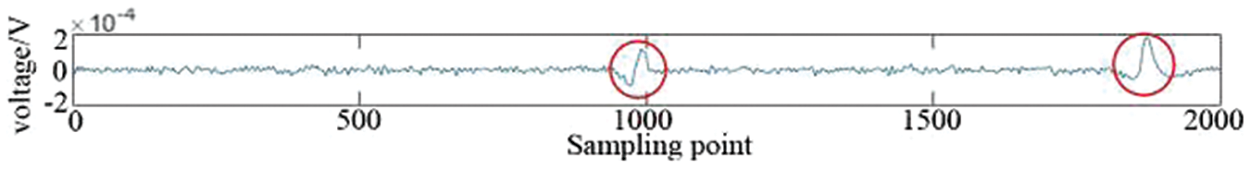
Figure 5: Typical electroocular artifact

The amplitude of EEG artifact is much larger than that of EEG, and its frequency band ranges from 0 to 16 Hz, while the EEG frequency band ranges from 0 to 32 Hz. Traditional filtering methods can not filter eye electrical signal artifacts effectively. The core step of the Hilbert Yellow transform [28] was the empirical mode decomposition of the signal, which adaptively decomposed signals into a series of intrinsic mode functions (IMF) [29]. Then, the Hilbert transform was expanded for each eigenmode function to obtain the instantaneous frequency of each component, and the signal was filtered according to the fast frequency. As shown in Fig. 6, multiple IMF components can be obtained by EMD decomposition of input signal X(t). In the first row, the original signal is EEG before filtering physiological artifacts, and IMF1 to IMF8 are component signals obtained after the empirical mode decomposition of the original signal. The processed signal is obtained after filtering out physiological artifacts from the original signal.

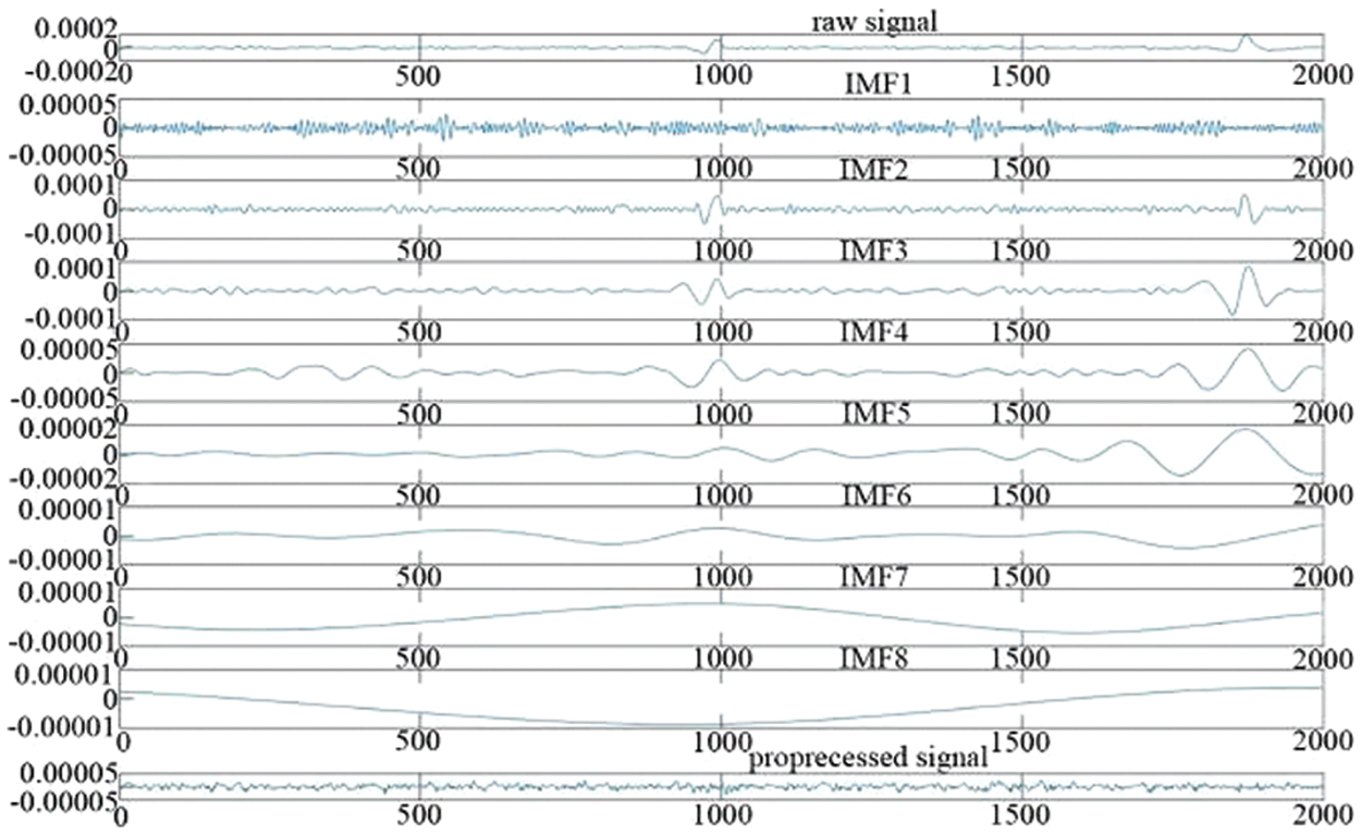
Figure 6: IMF component of EEG signal

For each IMF, its instantaneous frequency f(t) was calculated, and the fast frequency of the signal s(t)=α(t)cos⁡(ψt) was: f(t)=12πdd(t)[arg⁡z(t)].

The main frequency band of EEG signals is generally between 1–32 Hz, and the IMF component was filtered based on fast frequency:

si(t)={imfi(t),1≤fi(t)≤320,other(8)

where imfi is the i-th order eigenmode function of signal si(t) after EMD decomposition.

Significant jitters in signals caused by blinking and eye rotation were processed according to the standard deviation of the signal to eliminate significant jitters caused by eye electrical artifacts in signals. Processing rules are shown as follows:

xi(t)={si(t),|si(t)−mi|<λimiλi=mean|Pi−mi|+std|Pi−mi|(9)

where Pi is the sequence of extreme values of the i-th order IMF component, and mi is the mean value of the i-th order IMF component.

Then, filtered IMF components were linearly reconstructed to obtain new EEG signal h(t) as in h(t)=∑xi(t).

The reconstructed EEG signal waveform is shown in Fig. 7. The red dashed line is the raw EEG signal, and two physiological artifacts caused by blinking and eye rotation can be observed. The blue waveform represents the signal obtained after EMD decomposition and component filtering.

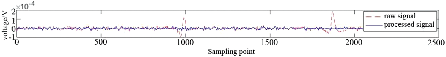
Figure 7: EEG signal waveform after filtering ocular electrical artifacts

2.2.2 Feature Extraction of EEG Signals

Physiological studies showed that information of each rhythm in prefrontal EEG was closely related to brain arousal degree [30]. δ rhythm is the primary frequency component of deep sleep. When the brain enters deep sleep, breathing gradually deepens, heart rate slows down, blood pressure and body temperature drop, and signal energy of EEG in the 1–4 Hz band increases significantly. θ rhythm is the primary frequency component of the brain during consciousness. ɑ wave is the primary frequency component of the brain when it is highly concentrated. β rhythm is the primary frequency component of the brain under anxiety and stress. However, due to the randomness and non-stationarity of EEG signals, the absolute frequency band energy intensity of EEG signals cannot accurately represent the brain state or cope with the uncertainty caused by individual differences. This paper used the Fourier transform [31] to convert it from the time domain to the frequency domain (Eq. (10)). Discrete EEG acquired directly by the acquisition device needs to be processed by discrete Fourier transform.

F(w)=∫−∞∞f(t)e−jwtdt(10)

Then, EEG signal characteristics based on frequency band energy ratio were adopted:

PSD(w)=|FFT(x(t))|2(11)

Ei=∑f−fi−minfi_maxPSD(w)(i=δ,θ,α,β)(12)

Rk=Ek∑Ei(i,k=δ,θ,α,β)(13)

2.2.3 Reflection Oxygen Saturation Calculation

Blood oxygen saturation (SpO2) refers to the percentage of actual dissolved oxygen content in human blood and the maximum oxygen content that can be dissolved in blood [32]. The formula of blood oxygen saturation was defined as follows:

SpO2=cHbO2cHbO2+cHb×100%(14)

CHb is deoxyhemoglobin, and CHbO2 is the concentration of oxygenated hemoglobin.

Studies have shown that the fluctuation range and distribution range of blood oxygen saturation of drivers in fatigued driving are more extensive than those in everyday driving [33]. Therefore, distribution characteristics can be obtained by statistics of blood oxygen saturation of drivers in daily driving and fatigue driving, represented by mean value (Eq. (15)) and standard deviation (Eq. (16)).

RAVG=1N∑i=1NRi(15)

RSD=1N−1∑i=1N(Ri−RAVG)2(16)

3  Research on Fatigue Analysis Method Based on Information Fusion

Among the most applied fatigue detection approaches, the method based on vehicle driving characteristics has low accuracy, prominent driving lanes, and poor night driving effect, so it is rarely used. Besides, in actual driving, image information captured in the driving environment is often affected by objective factors such as light and occlusion (glasses, hair obscuration), and the accuracy of detection based on eye features decreases. Therefore, to improve the accuracy and reliability of fatigue recognition, it is necessary to fuse images with biological signal features, which have significant changes and feature differences in the early fatigue stage.

Information fusion [34] is a comprehensive process of preprocessing, data registration, predictive estimation, and arbitration decision-making of information from similar or heterogeneous sources to obtain more accurate, stable, and reliable target information than a single source. Information fusion is mainly carried out from the following levels: Data layer fusion, feature layer fusion, and decision layer fusion.

3.1 Fatigue Detection Based on Feature Layer Fusion

In the driver fatigue detection scenario, various information sources can reflect the driver’s fatigue from different angles. Drivers’ facial information, biological signals, operating behavior information, and other characteristic indicators can well reflect drivers’ fatigue states from different perspectives to different degrees. Among them, drivers’ facial and physiological information are heterogeneous and have complementary characteristics. This multi-source heterogeneous information can be expanded from the feature and decision-level fusion. According to the principle of information fusion, combined with information features and the fusion purpose of this paper, feature fusion was carried out on multi-source information of face features and biometric features.

Feature layer fusion [35] refers to the preprocessing and feature extraction of raw data from each information source and then fusing features of each information source to obtain prediction and estimation of target information further. Commonly used feature-level fusion algorithms include neural networks, Multi-Kernel Learning (MKL), and typical Correlation Analysis (CA). MKL algorithm trained different kernel functions for additional features and then linearly weighted multiple kernel functions to obtain a combined kernel with multi-source information processing capability, which is suitable for multi-source heterogeneous information fusion. CA algorithm analyzed the intrinsic relationship between features by projecting features in the direction of maximum correlation to obtain new fused features, remove redundant information from features, and improve the ability of new features to represent target information.

3.1.1 Feature Fusion Based on Multi-Kernel Learning

By introducing the Kernel function, non-fractional data in input space was mapped to high-dimensional space. Then classification, clustering, and regression tasks were completed in high-dimensional space, called Kernel Methods or Kernel Machine [36]. A linearly indivisible feature vector x was made linearly separable by mapping it to another feature space through a function ϕ(x), where the classification hyperplane was f(x)=ωTϕ(x)+b, for any two samples xi and xj, the inner product in ϕ(x) space was k(xi,xj)=<ϕ(xi),ϕ(xj)>. Then k(xi,xj) was kernel function, and matrix k with elements k(xi,xj) was kernel matrix. Assuming that target information can be represented by M features, training data sample xi of target information was {x i1,xi2,…,xiM}, xit represented tth feature of sample i, where 1≤t≤M. Then for the tth feature, the basis kernel function was kt(xi,xj), the basis kernel matrix was Kt, and its nonlinear mapping function was ϕt(x). By a linear combination of multiple basis kernel functions, the combined kernel number kc was obtained as shown in Eq. (17), and the joint kernel matrix was established in the equation below:

kc=∑t=1Mαtkt(xit,xjt)(17)

Kc=∑t=1MαtKt(18)

where αt was the weight coefficient of the basis kernel kt and the nonlinear mapping function of the joint kernel was ϕc(x). Current research on base-core combination methods is mainly based on linear combinations. Although nonlinear combinations can give better results, the computational complexity is too high and the results are often difficult to interpret.

For M features of target information, each feature corresponded to at least one basis kernel, to construct basis kernel model kc, as shown in Fig. 8. The solution of structural parameters of the base kernel model (weight coefficients of the base kernel α={α1,α2,…,αM}) has become a hot research topic. MKL’s fusion ability was applied to fuse fatigue features from images and physiological information. With M kinds of fatigue features (denoted as x={x1,x2,…,xM}), we constructed a model of joint kernel based on radial basis function (RBF) kernel (the most widely used kernel) under the condition of uncertain distribution characteristics of each feature [37]. The formula of the RBF kernel is shown in Eq. (19). After determining the kernel function, we used an algorithm to train the weight coefficient of each basis kernel and inherent parameters of each basis kernel (parameter of RBF kernel function was σand σ>0), to obtain joint kernel kc. kc was then applied to various kernel methods to train classification/clustering/regression models.

k(xi,yj)=exp⁡(−‖xi−xj‖22σ2)(19)

Figure 8: Schematic diagram of multi-kernel learning

3.1.2 Feature Fusion Based on Multi-Set Canonical Correlation Analysis (MCCA)

For a feature set x=[x1,x2,…,xm] containing m features, the data dimension of feature xi was n. A linear transformation zi=xiwi was applied to each set of data, where wi was also known as projection direction. After the projection feature set z=[z1,z2,…,zm] was obtained, the projection directions were w=[w1,w2,…,wm], wT=[w1T,w2T,…,wmT]. After projection, the covariance matrix of feature set x and z were Cx=xTx and Cz=zTz, separately. The core task of MCCA was to find the appropriate projection of each feature set to maximize the correlation degree of each new feature in the projected feature set. SUMOR criterion [38] characterized correlation as the sum of all elements of Cz, then the problem was transformed into solving the following objective functions, the maximum value of wTCxw under constraints a and b. The objective function can then be solved using the Lagrange multiplier [39] to obtain the projection transformation matrix w=[w1,w2,…,wm].

max  wTCxw=∑i=1m∑j=1mwiTCijwjs.t. wiTCiiw=1, i=1,2,…,m  (a)  ∑i=1m(wiTCiiwi)=wTdiag(Cx)w=1, i=1,2,…,m(b)(20)

when m=2, MCCA was ordinary CCA. When m>2, MCCA analyzed comprehensive correlation degree between multiple features (feature sets). Feature set was obtained after the fusion of numerous feature sets.

3.1.3 Feature Layer Fusion Fatigue Detection Model

Features such as proportion of eyelid closure time per unit time (PERCLOS), blink frequency per unit time (BF), and mean eyelid ratio (ER) were extracted from driver’s face, and features such as ratio of each rhythm’s energy to total energy were extracted from driver’s EEG signals, which were used in combination with features of the mean and standard deviation of blood oxygenation saturation to characterize fatigue. Physical significance and dimensionality of eye-movement features and biosignal features extracted from driver facial information vary, with many feature parameters differing by orders of magnitude. Therefore, features need to be normalized before training. Normalization was performed using Eq. (21) to obtain normalized features for features in the sample.

αi ′=2αi−αmax−αminαmax−αmin,i=1,2,…,N(21)

where αi is a feature α of the ith sample, αmax, αmin are the maximum and minimum value of feature α among N samples.

For MCCA-based feature layer fusion, after feature normalization, MCCA was used to fuse features to obtain newly united features. MKL-based feature layer fusion assigned different kernel functions to additional features and received parameters and weights of each kernel function during model training. Both feature fusion methods applied SVM, and for kernel function, RBF kernel was chosen for model training. The machine learning library sklearn for Python has code implementations of SVM algorithms and interface functions for extended model training and testing. Code implementation of multi-core SVM algorithm is available in the machine learning library SHOGUN. In this paper, training for the driving fatigue detection model was carried out based on the above two tools. For SVM with RBF kernel, model parameters were penalty coefficient C and structural parameter σ of RBF kernel. For the training of the small-sample driving fatigue detection model, the grid search method was used to adjust parameters, limit the variation range and step size of the model parameters, and then exhaust all model parameter combinations to obtain the optimal parameters.

4  Experiment and Result Analysis

In this paper, simulated driving experiment was carried out on a driving simulation platform built by laboratory to simulate actual driving situations, and driver’s data was collected during simulated driving.

4.1 Experimental Platform

The experimental platform included a simulated driving platform and a data acquisition platform. A simulated driving platform was used to affect the driving situation. A data acquisition platform was used to collect multisource information synchronously. The experimental scenario is shown in Fig. 9a.

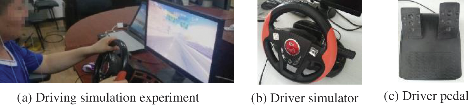
Figure 9: Driving simulation platform

4.1.1 Simulation Driving Experiment Platform

The driving simulation platform included driving simulation software, a view display, a steering wheel, a brake pedal, an accelerator pedal, and a host computer. Driving simulation software, called “City Car Driving,” provides a realistic reproduction of natural road scenes. The software ran on a PC and displayed traffic conditions through a monitor. Figs. 9b and 9c show the simulator used to deploy the driving simulation. When drivers apply torque to the steering wheel, the vehicle can give a corresponding degree of steering.

4.1.2 Data Acquisition Platform

A fatigue-driving monitoring device was designed for data acquisition of biosignals. A multifunctional and multi-node physiological parameter acquisition device obtained EEG and blood oxygen saturation signals. Data was transmitted to a host computer through Wi-Fi technology, which processed and analyzed data to get the fatigue status of the subject. The overall framework is shown in Fig. 10. CC3200 was the main control chip to control EEG and blood oxygen collection.

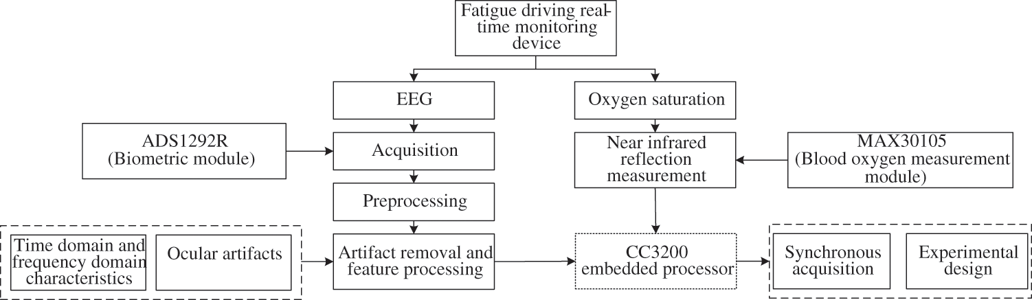
Figure 10: General framework of fatigue driving monitoring device

EEG signals of the brain’s different locations have different characteristics, distinguished according to the “10/20 international standard system”. The ADC for acquiring EEG signals was multi-channel and high-precision, with a sampling rate of 60 Hz. MAX30105 was used to measure blood oxygen saturation. Device nodes were placed on the head and earlobes when acquiring biosignals. Experimental equipment and specific connection modes are shown in Fig. 11.

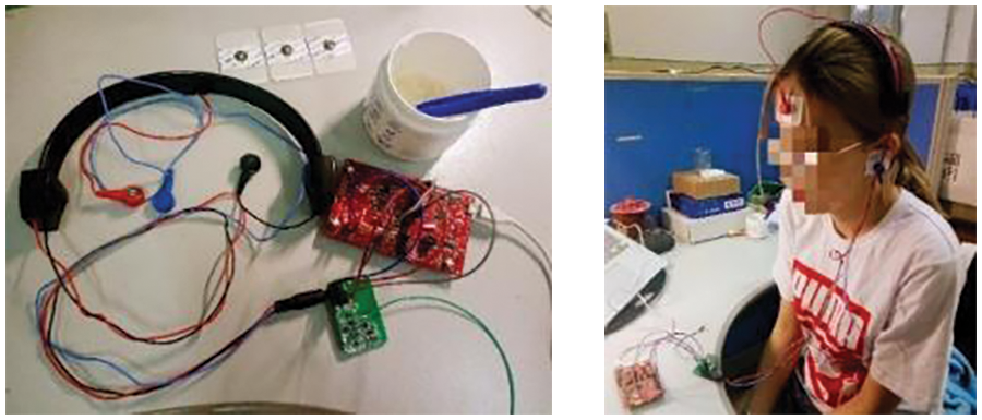
Figure 11: Experimental equipment and electrode lead mode

4.2 Paradigm of Experiment

The experimental environment was required to be a quiet and stable indoor environment, with sufficient light and no massive spatial electromagnetic interference, ensuring the acquisition of high-quality images and physiological signals. Ten participants were asked to be healthy, have no history of brain disease, and not consume stimulating beverages such as coffee and tea the day before the experiment. Meanwhile, subjects should be familiarized with the experimental procedure and equipment before the experiment. After experiment preparation, subjects were connected to an EEG and blood oxygen acquisition device and acquisition equipment; a camera was opened to ensure that the data acquisition platform could collect data properly. Then, the simulation driving software was turned on to make preparations. After that, experiments were conducted according to Experiments 1 and 2, respectively, for the data record.

(1) Simulated driving experiment (The collected data was labeled as Dataset 1)

The driving simulation experiment consisted of fatigue and non-fatigue driving experiments. The fatigue experiment required subjects to sleep for no more than seven hours and was conducted after lunch at 13:00 ~14:00 (when humans were prone to sleepiness) and during the night at 22:00–23:00. For non-fatigue experiments, subjects should ensure sufficient rest to maintain a good physical and mental state, and experiment time was 9:00–11:00. Subjects sat in driver’s seat and closed their eyes to calm down for 1 min. Afterward, driving simulation formally began, and the acquisition of drivers’ facial images and physiological information started simultaneously. Before the first experiment, participants were given three minutes to familiarize themselves with the driving simulator. The simulated driving time was 10 min.

(2) Reaction test experiment (The collected data was labeled as Dataset 2)

In the simulated driving process, drivers’ biological signals were collected, and drivers’ reaction time was recorded by synchronized stimulation with periodic fixed audio signals. After hearing the sound signal, drivers responded to the audio stimulus by pressing the button on the steering wheel. Reaction time can more accurately mark the degree of fatigue. A reaction time detection software was developed and run in the background to measure drivers’ reaction time. It has the following functions: (1) Send out audio periodically and record the time of the audio. (2) Detect whether the buttons on the steering wheel of simulated driving were pressed and record the pressing time of the keys. (3) Calculate the difference between audio sending time and critical pressing time, record differences, and save it as a CSV file. The interface diagram of the reaction time detection tool and program flow chart are shown in Figs. 12 and 13. The purpose of this reaction test is to automatically label collected driving data according to reaction time. Data from fatigue driving experiments were labeled based on synchronously collected reaction time. Reaction time was normalized to distribute between 0 and 1, where 0 is non-fatigue, and 1 is extreme fatigue.

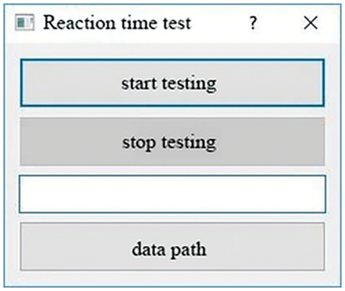
Figure 12: Reaction time detection interface

Figure 13: Flow chart of reaction time detection

4.3 Analysis of Experimental Data

After data collection, heterogeneous data from multiple information sources must be integrated into time series. In this experiment, the sampling frequency of biological signals was 60 Hz, and the camera’s frame rate was 30FPS. When data were aligned on time series, each second contained 60 points of biological information and 30 images of image information. When collating data sets, it is necessary to segment collected original data in time series, and the time window of segmentation is T, as shown in Fig. 14. The segmented data was used as a sample, and the sample was preprocessed to extract features.

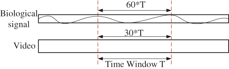
Figure 14: Schematic diagram of data alignment and segmentation

The size of window T significantly influenced PERCLOS and BF features in image information, and the blink interval of human eyes was about 3~4 s. However, the EEG signal artifact removal algorithm produces edge effects when processing short-term signals, and the time window T should not be too small. In this paper, original data were divided according to Windows of 3, 5, 7, 10, and 15 s, and the fatigue detection accuracy under different times Windows was discussed.

4.3.1 Effect Analysis of Fatigue Detection Based on Eye Movement Features

Two hundred eye movement sample features (including 100 eye movement sample features of drivers under fatigue driving and non-fatigue driving) were taken from Dataset 1. Each feature sample was extracted from video data samples of continuous 7 s, and 100 fatigue feature samples were obtained by segmenting constant 700 s fatigue driving video and extracting features piecewise.

(1) The distribution of PERCLOS characteristics is shown in Fig. 15. The Blue dotted line and red solid line were PERCLOS distribution of 100 fatigue and non-fatigue conditions. When the driver was tired, the distribution range of PERCLOS was significantly lower than that of a non-fatigue state.

Figure 15: Schematic diagram of PERCLOS feature distribution in fatigued/non-fatigued state

(2) Blink frequency distributions are shown in Fig. 16. The Blue dashed and red solid lines indicated blink frequency distribution of 100 fatigued and 100 non-fatigued samples. It can be observed that when the driver was tired, the blink frequency oscillated violently before 0 and higher values. This is because when drivers realized they were tired, they suddenly blinked quickly and tried to stay awake.

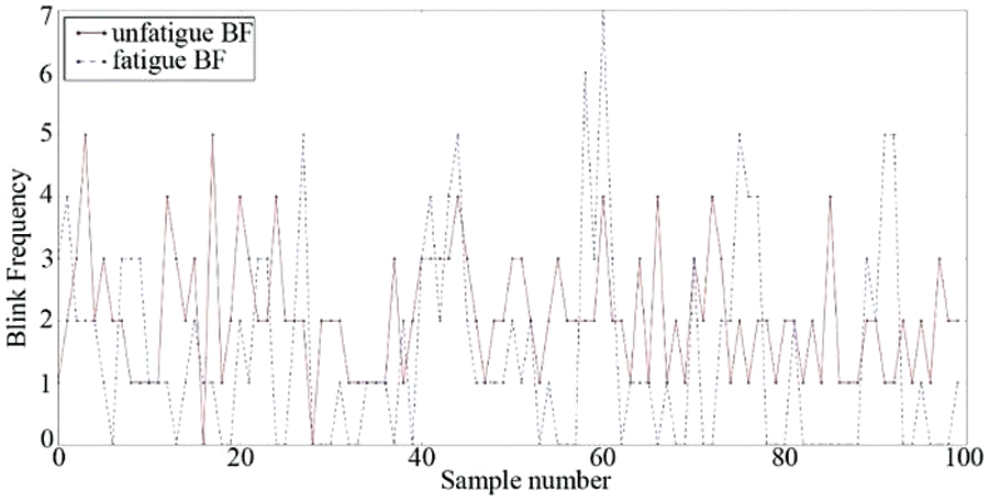
Figure 16: Schematic diagram of eyeblink frequency distribution in fatigue/non-fatigue state

(3) In Fig. 17, the solid red line was the ER feature extracted from 700 s continuous fatigued driving video screens, and the dashed blue line was the feature extracted from 700 s continuous non-fatigued driving video screens. The mean eyelid opening was significantly higher in the sleepy state than in the non-fatigued one. This indicated that ER characteristics can represent a fatigue state.

Figure 17: Average eyelid height/width ratio under fatigue/non-fatigue condition

By comparing the above features, it is possible to analyze the ability of these features to characterize the fatigue state to varying degrees. The above three features were formed into a 3-dimensional feature vector as sample features from image information. The fatigue driving detection model was trained based on SVM, and model parameters were adjusted by grid search. Detection accuracy based on the time window of 3, 5, 7, 10, 15 s were 74.6%, 82.8%, 86.1%, 85.6%, 87.3%, separately. The size of the time window impacted the accuracy rate of recognition. The main reason for the difference was that the three eye movement features were all based on time series statistics, and the change patterns of these features each have their period (for example, the blink frequency of normal people is generally 3–4 s). Extracted features will be greatly affected when the time window exceeds this period. Therefore, the time window should not be too small when extracting eye movement features from image information.

4.3.2 Effect Analysis of Fatigue Detection Based on EEG Features

Two hundred sets of EEG samples were taken from experimental Dataset 1, including 100 fatigue EEG samples and 100 non-fatigue samples. Each sample contained power spectral-based features extracted from a continuous period of 7 s of EEG signals. The feature component is a four-dimensional feature based on the power spectrum of each rhythm. To further directly analyze the relationship between the energy ratio of each rhythmic band of the driver’s EEG signals and fatigue, EEG signals of FP1 were collected. The energy conversion calculation for each rhythm is shown in Fig. 18. It can be observed that when the driver gradually entered drowsiness, unconsciousness, or even sleep state, the energy ratio of δ and θ rhythm rose rapidly. In contrast, the energy of ɑ and β rhythm quickly decreased, which was consistent with medical research results: δ and θ rhythm indicated inhibition degree of specific neurons in the cerebral cortex, while ɑ and β rhythm indicated excitation degree of neurons in the cerebral cortex.

Figure 18: Change of energy ratio of EEG signal rhythm

Power spectrum features of EEG signals were combined to form a 4-dimensional feature vector, and feature samples of EEG signals were organized. SVM was used to train the driving fatigue detection model based on EEG signals, and grid search was used to adjust model parameters to obtain the fatigue driving detection model. Classification accuracy based on time window of 3, 5, 7, 10, 15 s, were 74.2%, 72.4%, 81.8%, 71.6%, 76.4%, separately. EEG was not sensitive to time window size and did not affect accuracy because features extracted from EEG were all power spectral features belonging to the frequency domain and were not directly affected as image features extracted from time series.

4.3.3 Driving Fatigue Evaluation Method Based on Blood Oxygen

Changes in blood oxygen saturation under everyday driving and fatigue driving conditions are shown in Fig. 19. It can be observed that the fluctuation range and distribution range of blood oxygen saturation of fatigued driving were more extensive than those of daily driving.

Figure 19: Blood oxygen saturation in different states

According to research on driving fatigue evaluation methods based on blood oxygen [40], changes in blood oxygen saturation standard deviation in two states can determine fatigue. The distribution of standard deviation of blood oxygen during daily and tired driving is shown in Fig. 20.

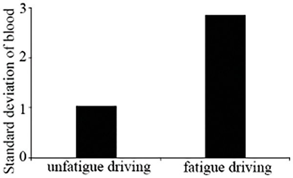
Figure 20: Distribution of standard deviation of blood oxygen under different driving states

The standard deviation of blood oxygen in fatigued driving was higher than that of daily driving, so the increase in blood oxygen standard deviation can be used to judge driving fatigue.

4.3.4 Comparative Analysis of Experimental Data

Single-mode driving fatigue detection methods and information fusion-based fatigue driving detection methods were evaluated using the experimental dataset. Detection effectiveness of the various techniques is shown in the following table. Data sets in Table 2 were divided by time window T = 7.

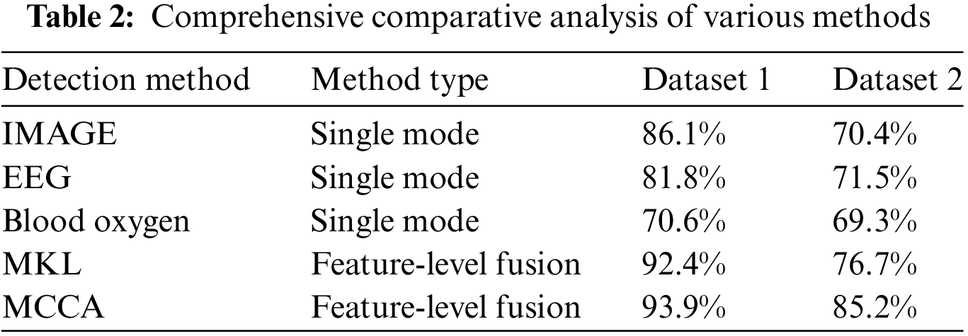
MKL and MCCA represented driving fatigue detection methods based on separately fused MKL and MCCA feature layers. By comparing experimental results, we can conclude that:

(1) Accuracies of the experiments conducted on Dataset 1 were generally much higher than that of Dataset 2, suggesting that the simulated driving data collected through Experiment 1 and the fatigued/non-fatigued driving labeling method were more reasonable. Experiment 1 ensured that the experimenter entered a sleepy state, accurately collected fatigue driving data, and established a fatigued/non-fatigued dataset. However, the reaction time was random, and the experimental method based on reaction time had a specific interference with simulated driving.

(2) Comparing the IMG single-mode driving fatigue detection method with the physiological signal detection method in Table 2, it can be found that the driving fatigue detection method based on drivers’ eye movement characteristics was significantly higher than physiological signal characteristics in Dataset 1. Drivers had apparent drowsiness, and eye features were substantially different from those in non-fatigue states. Under ideal conditions, driving fatigue detection based on image information can obtain better results. However, due to the difficulty of signal acquisition, physiological artifacts cannot be wholly filtered, and the accuracies of physiological signals were lower than that of image information. However, in real driving scenarios, fatigue is a slowly changing signal; drivers will gradually develop prominent fatigue characteristics only when driving fatigue accumulates to a certain degree and thus enters a state of profound fatigue. Moving fatigue will be reflected in physiological information first and then gradually show characteristics of eye fatigue. When drivers began to show apparent eye fatigue features, drivers were already in an over-fatigued state, which would be very dangerous. Therefore, the combination of images and physiological information is essential and should be acted upon as soon as it is observed that the driver is beginning to feel tired.

(3) By comparing driving fatigue detection results, it can be seen that the information fusion algorithm did improve fatigue driving detection accuracy to some extent, but at the expense of some efficiency. Compared with only using image-based algorithms, the efficiency was slightly reduced. In addition to time efficiency issues, the detection effect based on Datasets 1 and 2 has been improved by information fusion. Among them, the results of the MCCA-based feature layer fusion method were better. MCCA fused multiple features by analyzing the correlation between features, using two main features of information fusion: Information complementarity and information redundancy.

5  Conclusion

Driving is a complex, multifaceted, and potentially risky activity that requires total mobilization and utilization of physiological and cognitive abilities. Driver sleepiness, fatigue, and inattention are significant causes of road traffic accidents, leading to sudden deaths, injuries, high mortality rates, and economic losses. Sleepiness, often caused by stress, fatigue, and illness, reduces cognitive abilities, which affects drivers’ skills and leads to many accidents. Road traffic accidents related to sleepiness are associated with mental trauma, physical injury, and death and are often accompanied by economic losses. Sleeping-related crashes are most common among young people and night shift workers. Accurate driver sleepiness detection is necessary to reduce the driver sleepiness accident rate. Many researchers have tried to detect the sleepiness of a system using different characteristics related to vehicles, driver behavior, and physiological indicators. Among the most applied methods, the method based on vehicle driving characteristics has low accuracy and poor night driving effect, so it is rarely used. Besides, in actual driving, image information captured in the driving environment is often affected by objective factors such as light and occlusion (glasses, hair obscuration), and the accuracy of detection based on eye features decreases. Furthermore, in real driving scenarios, fatigue is a slowly changing signal, and drivers will gradually show prominent fatigue characteristics only when driving fatigue accumulates to a certain degree, thus entering a state of profound fatigue. Moving fatigue will first be reflected in physiological information and then gradually show the characteristics of eye fatigue. Consequently, detection methods of drivers’ fatigue have gradually diversified from original detection methods based on the driver’s facial image information to those found in physiological details such as EEG, respiratory pulse, and blood oxygen. However, the fatigue state of drivers is easily affected by their own body and interference with the external environment, which brings many problems to the reliability of fatigue driving detection. Physiological signals provide information about the body’s internal functioning, thus providing accurate, reliable, and robust information about the state of drivers.

This paper studied driving fatigue detection methods based on single-mode and multisource information (fusion of image and physiological information) by analyzing domestic and foreign research on fatigue detection technology. Simulated driving experiments were designed to evaluate and compare various driving fatigue detection methods, improving the accuracy, stability, and environmental adaptability of driving fatigue detection. A fatigue feature extraction method based on the driver’s facial information (eye-movement features) was explored, and the eye-movement feature parameters representing the driver’s fatigue level under fatigue and non-fatigue conditions, such as the percentage of eye closure time and the blinking frequency were investigated. Following that, the fatigue driving detection model was trained based on eye movement features to categorize fatigue state and non-fatigue state, with an accuracy of 86%. In addition, based on the designed portable fatigue driving monitoring device, a multi-sensor acquisition network was used to detect multiple physiological parameters (EEG and blood oxygen) information synchronously, and data-adaptive operation was carried out at the detection end to realize validity discrimination of measured signals. The energy ratio of each rhythm band, representing the degree of fatigue, was extracted from EEG signals and physiological signal characteristics such as the standard deviation of blood oxygen. The driver fatigue detection model was trained to classify the fatigue and non-fatigue states, and the accuracy rate reached 82%. Various experiments were conducted based on the simulation driving experiment platform. Facial information and biosignals of drivers during driving were collected simultaneously. Data were then segmented and labeled to obtain a driving database, including fatigue driving data and non-fatigue driving data, which was used to evaluate detection effectiveness. Afterward, feature layer information fusion methods based on MKL and MCCA were used to fuse various eye movements and physiological features. The driving fatigue detection model was trained based on the fused features, and the accuracy reached 92% and 94%, respectively. In summary, the wider the feature coverage is, the more accurate and reliable the driver fatigue detection results will be.

Although fatigue driving was studied from image and physiological information sources, more information sources (such as ECG signals, EMG signals, driving behavior information, and vehicle information) can also be added to improve the accuracy and stability of driving fatigue detection. The experiments in this paper are based on the existing laboratories and have many limitations. In the future, a better and more scientific experimental platform can be built, and more professional drivers can be recruited to conduct experiments, collect a large number of driving data, and support research ongoing fatigue detection methods. In addition, based on the research in this paper, the development of the implementation of intelligent accident prevention systems is worth looking forward to. Among them, the tremendous growth of wearable sensors, especially flexible sensors in biochemical signal measurement, provides technical support for the long-term dynamic measurement of multimodal signals of weak physiological signals of fatigue driving. This is an essential direction for wearable driver fatigue recognition. In the future, research on driver fatigue state recognition based on biosignal characteristics can be carried out by relying on low-invasion and high-popularity smartwatches.

Acknowledgement: Not applicable.

Funding Statement: This work was sponsored by the Fundamental Research Funds for the Central Universities (Grant No. IR2021222) received by J.S and the Future Science and Technology Innovation Team Project of HIT (216506) received by Q.W.

Author Contributions: The authors confirm their contribution to the paper as follows: study conception and design: Meiyan Zhang, Boqi Zhao; data collection: Jipu Li; analysis and interpretation of results: Qisong Wang; draft manuscript preparation: Dan Liu, Jingxiao Liao. All authors reviewed the results and approved the final version of the manuscript.

Availability of Data and Materials: SHOGUN toolkit is linked to http://www.shogun-toolbox.org/.

Conflicts of Interest: The authors declare that they have no conflicts of interest to report regarding the present study.

References

1. A. B. A. Al-Mekhlafi, A. S. N. Isha, and G. M. A. Naji, “The relationship between fatigue and driving performance: A review and directions for future research,” J. Crit. Rev., vol. 7, no. 14, pp. 134–141, Jul. 2020. doi: 10.31838/jcr.07.14.24. [Google Scholar] [CrossRef]

2. Y. Al-Wreikat, C. Serrano, and J. R. Sodré, “Driving behaviour and trip condition effects on the energy consumption of an electric vehicle under real-world driving,” Appl. Energy, vol. 297, pp. 117096, May 2021. doi: 10.1016/j.apenergy.2021.117096. [Google Scholar] [CrossRef]

3. H. Singh and A. Kathuria, “Analyzing driver behavior under naturalistic driving conditions: A review,” Accid. Anal. Prev., vol. 150, no. 2, pp. 105908, Dec. 2020. doi: 10.1016/j.aap.2020.105908. [Google Scholar] [PubMed] [CrossRef]

4. A. N. Abdelhadi, “Application of Toyota’s production system to reduce traffic accidents in Abha’s region-case study,” in Proc. ICIEOM, Bali, Indonesia, Jan. 2014, pp. 7–9. [Google Scholar]

5. K. Khan, S. B. Zaidi, and A. Ali, “Evaluating the nature of distractive driving factors towards road traffic accident,” Civ. Eng. J., vol. 6, no. 8, pp. 1555–1580, Aug. 2020. doi: 10.28991/cej-2020-03091567. [Google Scholar] [CrossRef]

6. M. K. Hussein, T. M. Salman, A. H. Miry, and M. A. Subhi, “Driver drowsiness detection techniques: A survey,” in Proc. BICITS, Babil, Iraq, Aug. 2021, pp. 45–51. [Google Scholar]

7. R. Lu, B. Zhang, and Z. Mo, “Fatigue detection method based on facial features and head posture,” J. Sys. Simul., vol. 34, no. 10, pp. 2279–2292, 2022. [Google Scholar]

8. A. Balasundaram, S. Ashokkumar, D. Kothandaraman, K. SeenaNaik, E. Sudarshan and A. Harshaverdhan, “Computer vision based fatigue detection using facial parameters,” IOP Conf. Ser.: Mater. Sci. Eng., vol. 981, no. 2, pp. 022005, 2020. doi: 10.1088/1757-899X/981/2/022005. [Google Scholar] [CrossRef]

9. H. Garg, “Drowsiness detection of a driver using conventional computer vision application,” in Proc. PARC, Mathura, India, Aug. 2020, pp. 50–53. [Google Scholar]

10. R. B. Wang, K. Y. Guo, and J. W. Chu, “Research on eye positioning method for driver fatigue monitoring,” J. Highway Traffic Sci. Technol., vol. 20, no. 5, pp. 111–114, 2003. doi: 10.3969/j.issn.1002-0268.2003.05.029. [Google Scholar] [CrossRef]

11. M. Ye, W. Zhang, P. Cao, and K. G. Liu, “Driver fatigue detection based on residual channel attention network and head pose estimation,” Appl. Sci., vol. 11, no. 19, pp. 9195, Oct. 2021. doi: 10.3390/app11199195. [Google Scholar] [CrossRef]

12. A. A. Saleem, H. U. R. Siddiqui, M. A. Raza, F. Rustam, S. Dudley and I. Ashraf, “A systematic review of physiological signals based driver drowsiness detection systems,” Cogn. Neurodyn., vol. 17, no. 5, pp. 1229–1259, Oct. 2023. doi: 10.1007/s11571-022-09898-9. [Google Scholar] [PubMed] [CrossRef]

13. M. Thilagaraj, M. P. Rajasekaran, and U. Ramani, “Identification of drivers drowsiness based on features extracted from EEG signal using SVM classifier,” 3C Tecnologia, pp. 579–594, 2021. doi: 10.17993/3ctecno.2021.specialissue8.579-595. [Google Scholar] [CrossRef]

14. C. Lv, J. Nian, Y. Xu, and B. Song, “Compact vehicle driver fatigue recognition technology based on EEG signal,” IEEE Trans. Intell. Transport. Syst., vol. 23, no. 10, pp. 19753–19759, 2021. doi: 10.1109/TITS.2021.3119354. [Google Scholar] [CrossRef]

15. C. N. Watling, M. M. Hasan, and G. S. Larue, “Sensitivity and specificity of the driver sleepiness detection methods using physiological signals: A systematic review,” Accid. Anal. Prev., vol. 150, no. 4, pp. 105900, 2021. doi: 10.1016/j.aap.2020.105900. [Google Scholar] [PubMed] [CrossRef]

16. S. Murugan, J. Selvaraj, and A. Sahayadhas, “Detection and analysis: Driver state with electrocardiogram (ECG),” Phys. Eng. Sci. Med., vol. 43, no. 2, pp. 525–537, Jun. 2020. doi: 10.1007/s13246-020-00853-8. [Google Scholar] [PubMed] [CrossRef]

17. P. Sugantha Priyadharshini, N. Jayakiruba, A. D. Janani, and A. R. Harini, “Driver’s drowsiness detection using SpO2,” in Proc. BDCC, Cham: Springer Nature Switzerland, Jun. 2022, pp. 207–215. [Google Scholar]

18. J. C. Sun, Z. L. Yang, C. Shen, S. Cheng, J. Ma and W. D. Hu, “Mental fatigue state of brain tissue oxygen saturation of near-infrared spectral analysis,” Modern Biomed. Prog., vol. 15, no. 34, pp. 6697–6700, 2015. doi: 10.13241/j.cnki.pmb.2015.34.024. [Google Scholar] [CrossRef]

19. Z. Li, L. Chen, L. Nie, and S. X. Yang, “A novel learning model of driver fatigue features representation for steering wheel angle,” IEEE Trans. Veh. Technol., vol. 71, no. 1, pp. 269–281, 2021. doi: 10.1109/TVT.2021.3130152. [Google Scholar] [CrossRef]

20. S. Ansari, H. Du, F. Naghdy, and D. Stirling, “Automatic driver cognitive fatigue detection based on upper body posture variations,” Expert Syst. Appl., vol. 203, no. 2, pp. 117568, 2022. doi: 10.1016/j.eswa.2022.117568. [Google Scholar] [CrossRef]

21. M. Peivandi, S. Z. Ardabili, S. Sheykhivand, and S. Danishvar, “Deep learning for detecting multi-level driver fatigue using physiological signals: A comprehensive approach,” Sens., vol. 23, no. 19, pp. 8171, Sep. 2023. doi: 10.3390/s23198171. [Google Scholar] [PubMed] [CrossRef]

22. O. Déniz, G. Bueno, J. Salido, and F. de la Torre, “Face recognition using histograms of oriented gradients,” Pattern Recogn. Lett., vol. 32, no. 12, pp. 1598–1603, Jan. 2011. doi: 10.1016/j.patrec.2011.01.004. [Google Scholar] [CrossRef]

23. J. Hosang, R. Benenson, and B. Schiele, “Learning non-maximum suppression,” in Proc. ICVPR, vol. 2017, 2017, pp. 4507–4515. [Google Scholar]

24. K. Trejo and C. Angulo, “Single-camera automatic landmarking for people recognition with an ensemble of regression trees,” Comput. Y Sist., vol. 20, no. 1, pp. 19–28, 2016. doi: 10.13053/cys-20-1-2365. [Google Scholar] [CrossRef]

25. J. Brophy, Z. Hammoudeh, and D. Lowd, “Adapting and evaluating influence-estimation methods for gradient-boosted decision trees,” J. Mach. Learn. Res., vol. 24, no. 154, pp. 1–48, 2023. doi: 10.48550/arXiv.2205.00359. [Google Scholar] [CrossRef]

26. D. E. King, “Dlib-ml: A machine learning toolkit,” J. Mach. Learn. Res., vol. 2009, no. 10, pp. 1755–1758, 2009. doi: 10.5555/1577069.1755843. [Google Scholar] [CrossRef]

27. X. Jiang, G. B. Bian, and Z. Tian, “Removal of artifacts from EEG signals: A review,” Sens., vol. 19, no. 5, pp. 987, 2019. doi: 10.3390/s19050987. [Google Scholar] [PubMed] [CrossRef]

28. N. E. Huang, “Hilbert-Huang transform and its applications,” World Sci., vol. 16, pp. 1–400, 2014. doi: 10.1142/IMS. [Google Scholar] [CrossRef]

29. R. C. Sharpley and V. Vatchev, “Analysis of the intrinsic mode functions,” Constr. Approx., vol. 24, no. 1, pp. 17–47, 2006. doi: 10.1007/s00365-005-0603-z. [Google Scholar] [CrossRef]

30. P. Halász, M. Terzano, L. Parrino, and R. Bódizs, “The nature of arousal in sleep,” J. Sleep Res., vol. 13, no. 1, pp. 1–23, 2004. doi: 10.1111/j.1365-2869.2004.00388.x. [Google Scholar] [PubMed] [CrossRef]

31. J. W. Cooley, P. A. W. Lewis, and P. D. Welch, “The fast Fourier transform and its applications,” IEEE Trans. Educ., vol. 12, no. 1, pp. 27–34, 1969. doi: 10.1109/TE.1969.4320436. [Google Scholar] [CrossRef]

32. D. J. Faber, E. G. Mik, M. C. G. Aalders, and T. G. van Leeuwen, “Toward assessment of blood oxygen saturation by spectroscopic optical coherence tomography,” Opt. Lett., vol. 30, no. 9, pp. 1015–1017, 2005. doi: 10.1364/OL.30.001015. [Google Scholar] [PubMed] [CrossRef]

33. M. A. Kamran, M. M. N. Mannan, and M. Y. Jeong, “Drowsiness, fatigue and poor sleep’s causes and detection: A comprehensive study,” IEEE Access, vol. 7, pp. 167172–167186, 2019. doi: 10.1109/ACCESS.2019.2951028. [Google Scholar] [CrossRef]

34. A. Ross and A. Jain, “Information fusion in biometrics,” Pattern Recogn. Lett., vol. 24, no. 13, pp. 2115–2125, 2003. doi: 10.1016/S0167-8655(03)00079-5. [Google Scholar] [CrossRef]

35. S. Kiran et al., “Multi-layered deep learning features fusion for human action recognition,” Comput. Mater. Contin., vol. 69, no. 3, pp. 4061–4075, 2021. doi: 10.32604/cmc.2021.017800. [Google Scholar] [CrossRef]

36. M. Gönen and E. Alpaydın, “Multiple kernel learning algorithms,” J. Mach. Learn. Res., vol. 12, pp. 2211–2268, 2011. [Google Scholar]

37. J. Ghosh and A. Nag, “An overview of radial basis function networks,” New Adv. Des., vol. 2001, pp. 1–36, 2001. [Google Scholar]

38. L. Wang, Y. Shi, and H. B. Ji, “Fingerprint identification of radar emitter based on multi-set canonical correlation analysis,” J. Xidian Univ., vol. 40, no. 2, pp. 164–171, 2013. doi: 10.3969/j.issn.1001-2400.2013.02.027. [Google Scholar] [CrossRef]

39. Y. O. Li, T. Adali, W. Wang, and V. D. Calhoun, “Joint blind source separation by multi-set canonical correlation analysis,” IEEE Trans. Signal Process., vol. 57, no. 10, pp. 3918–3929, Oct. 2009. doi: 10.1109/TSP.2009.2021636. [Google Scholar] [PubMed] [CrossRef]

40. K. Mohanavelu, R. Lamshe, S. Poonguzhali, K. Adalarasu, and M. Jagannath, “Assessment of human fatigue during physical performance using physiological signals: A review,” Biomed. Pharmacol. J., vol. 10, no. 4, pp. 1887–1896, 2017. doi: 10.13005/bpj/1308. [Google Scholar] [CrossRef]