Safety-Constrained Multi-Agent Reinforcement Learning for Power Quality Control in Distributed Renewable Energy Networks

1  Introduction

The conventional utilization of non-renewable energy sources for electricity generation has given rise to issues of energy scarcity and environmental pollution. To address these concerns, an increasing reliance on renewable energy sources, such as solar and wind power, has been observed in power generation. However, the intermittent and volatile nature of renewable energy sources poses significant challenges to the safe operation and stability of the electrical grid when integrated into it. Within the grid, it is imperative to maintain specific ranges of both frequency and voltage to ensure the normal operation of various devices. Frequent fluctuations and unstable power supply can result in power quality issues, including voltage fluctuations, harmonics, and intermittent power supply, which may adversely affect grid stability and impact sensitive electronic equipment and industrial processes [1]. This article primarily explores how to mitigate the instability of renewable energy-based electricity generation through voltage control. Active power voltage control involves the adjustment of the active power level within the electrical system to ensure that the grid voltage is maintained within suitable limits. This can be achieved through the adjustment of generator output, the utilization of reactive power compensation devices (such as synchronous condensers or capacitors), and the implementation of voltage stabilizers to alleviate issues related to overvoltage and undervoltage [2].

Active power voltage control has always played a crucial role in traditional distribution grids. However, with the increasing integration of distributed renewable energy sources into the grid, an excessive injection of active power may lead to voltage fluctuations beyond the prescribed thresholds in the grid [3]. This renders traditional control algorithms, such as droop control and optimal power flow (OPF) [4], less adaptable to the uncertainty in distributed renewable energy networks. Droop control is a relatively simple control strategy that does not necessitate complex optimization algorithms or communication systems. Nevertheless, the parameters of droop control are typically fixed, making it less responsive to changes in grid conditions. On the other hand, OPF offers flexibility by adjusting to grid requirements and operational constraints, but it relies on intricate mathematical models and computations, often demanding high-performance computing and real-time data updates. Active power voltage control problem exhibits two primary characteristics: (1) In a distributed network, voltage is influenced by neighboring nodes, and as the distance between nodes increases, the likelihood of mutual influence decreases. (2) It presents a constrained multi-objective optimization problem, where the objective is to maintain the voltage within prescribed limits for all buses while minimizing total power losses [5].

Multi-agent reinforcement learning (MARL) is a subfield of reinforcement learning that involves multiple intelligent agents operating in a shared environment, learning to make decisions that maximize their individual long-term cumulative rewards. Each agent acts as an independent learning entity, but their behaviors interact with and influence each other since they share the environment and may pursue common or competitive objectives. MARL typically encompasses cooperative collaboration and competitive rivalry, addressing complex issues of coordination, communication, and competition. In the context of the power system, distributed voltage control is a critical concern for ensuring grid stability and voltage quality. Conventional voltage control methods typically involve centralized control or rule-based local control, which may lack the flexibility and efficiency needed in complex distributed energy environments. Consequently, the application of MARL holds significant potential in the realm of distributed voltage control [6].

Currently, many research efforts aim to employ MARL to address the issue of distributed voltage control [6–10]. Each of these studies has demonstrated that MARL-based approaches outperform traditional control algorithms. However, most of these works have not considered large-scale power grids. To assess the performance of MARL, this paper utilizes three power grids of varying scales, which can be employed to validate the effectiveness of MARL in different grid sizes and identify MARL algorithms suitable for voltage control. While MARL surpasses traditional algorithms in the context of distributed voltage control, it frequently exhibits risky actions during the early training and transfer processes, thereby increasing the risk of grid failure. Therefore, to ensure the safety of MARL throughout its training, testing, and transfer phases, this paper proposes the inclusion of safety constraints on MARL to guarantee both secure actions and the safe operation of the power grid. The primary contributions of this paper are as follows:

1.    In response to voltage control, we propose safety-constrained multi-agent reinforcement learning (SC-MARL) based on MARL. SC-MARL integrates a safety constraint module to derive secure actions, ensuring the safety of MARL-controlled actions during the voltage control process.

2.    We conducted a comparative analysis of various MARL algorithms and the SC-MARL algorithm. Experimental results demonstrate that, in contrast to other MARL algorithms, SC-MARL consistently ensures the generation of safe actions. Moreover, throughout the training and testing phases, the proportion of voltage exceeding the safety range approaches zero.

3.    Our experiments involved three different scales of power grids: 33-buses, 141-buses, and 322-buses. SC-MARL exhibited optimal performance across all three power grids, underscoring its adaptability as the scale of the power grid expands.

The remainder of this paper is organized as follows. Section 2 describes the work related to traditional methods and MARL for active voltage control. Section 3 formulates the power quality control problem and solves it using safety-constrained MARL. The experiments and results are described in detail in Section 4. Finally, we summarize our work in Section 5.

2  Related Work

Traditional distribution networks typically have few or no renewable energy generation nodes, and voltage control is primarily managed through voltage control devices such as static var compensators (SVCs) and on-load tap changers (OLTCs) [11]. These voltage control devices are often installed at substations, limiting their control to the voltages at these substations, while more distant nodes or buses are not effectively regulated [12]. The integration of many photovoltaic (PV) into the grid has raised interest in controlling the reactive power output of PVs to adjust the voltages at their respective buses. In this context, methods such as OPF and droop control are frequently employed to address voltage control issues. OPF is typically considered in two main variants: Centralized OPF [13] and distributed OPF [14]. Centralized OPF primarily addresses the problem of minimizing overall power losses, while distributed OPF aims to decentralize using the alternating direction method of multipliers (ADMM) to enhance computational efficiency. However, OPF’s primary limitation is its inability to achieve real-time control in dynamic power systems, particularly in rapidly changing voltage scenarios [15]. On the other hand, droop control is often employed for local voltage control, offering strong real-time responsiveness. Yet, distributed networks require communication to enable global voltage stability [16]. In summary, while OPF can minimize power losses, it lacks real-time responsiveness, and droop control offers real-time capabilities but does not optimize power losses. Therefore, this paper adopts MARL to learn voltage control strategies, striking a balance between real-time responsiveness and power loss minimization.

MARL is increasingly being applied by researchers to address the issue of active voltage control. Commonly used MARL algorithms in research include multi-agent deep deterministic policy gradient (MADDPG) [8], multi-agent soft actor critic (MASAC) [17], and multi-agent twin delayed deep deterministic policy gradient algorithm (TD3) [7], among others. These studies typically divide the distributed renewable energy network into numerous regions, with each region having a single agent. Each agent can manipulate the reactive power to affect the active power, with a focus on central training and decentralized execution (CTDE) frameworks. CTDE has the advantage of allowing each agent to learn global information and then execute actions quickly at the local level. However, these studies do not account for scenarios in which a region contains multiple agents or when the network scales up. To address these issues, a team led by A models the active voltage control problem as a decentralized partially observable markov decision process (Dec-POMDP) [18], in which each region contains multiple PV inverters. The control objective is to regulate the active power by adjusting the reactive power of each inverter. Additionally, they evaluate the performance of various MARL algorithms in three different scales of power networks [19]. Nonetheless, a common limitation of MARL algorithms is their failure to consider security concerns during training, testing, and transfer learning.

In the context of power grids, operational safety is of paramount importance, as actions that exceed safety boundaries can potentially lead to grid failures. Therefore, ensuring the safety of MARL involves agents maximizing rewards while simultaneously ensuring that their actions comply with safety requirements. One approach to ensuring the safety of MARL is by designing a safe reward function that encourages MARL to favor actions with high rewards. However, this does not guarantee safety during the model training phase [20]. To ensure safety during the training phase, the constrained policy optimization method can be employed, which restricts the policy’s single-step updates through trust region optimization [21]. Nonetheless, this approach does not guarantee safety during the agent’s testing phase. The utilization of Lyapunov functions, which guide policy learning, can provide safety assurance for both training and testing phases, but it is limited to global safety. To enable agents to take safe actions during training, testing, and transfer learning, we propose a safety-constrained MARL method. This primarily involves calculating safe actions by taking derivatives with respect to each action through the observed voltage changes, facilitated by the Lyapunov functions.

3  Methodology

3.1 Distributed Renewable Energy Network

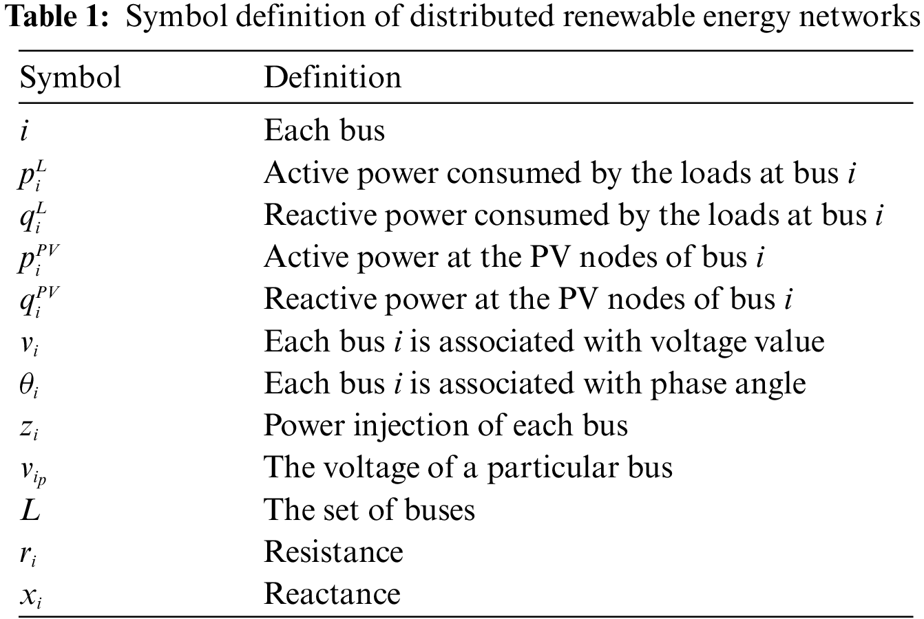
The distributed renewable energy network is primarily divided into three components: Generation, transmission, and local renewable energy systems, as illustrated in Fig. 1. Power generation involves the utilization of sources such as hydro energy, nuclear energy, and thermal energy. To minimize losses during the generation and transmission process, high voltages are often employed. The transmission component transports and distributes the electricity generated by power plants to residential or industrial consumers. To meet users’ electricity demands, voltage is adjusted to accommodate the load through transformers. In this paper, renewable energy primarily refers to solar energy. Solar panels are not mandatory on the user side, so solar farms are introduced to address this issue. Local management entities communicate with users, solar farms, and smart meters through a network to obtain power parameter information. Solar power cannot be directly injected into the grid and requires conversion through voltage transformers. Due to the intermittent nature of solar power generation, voltage instability occurs on the user side, with the risk of voltage exceeding safe levels and causing reverse current flow into the grid. After acquiring power information, local management entities control the reactive power of the PV voltage converter to adjust the voltage within a safe range. Symbol definition of distributed renewable energy networks are shown in Table 1.

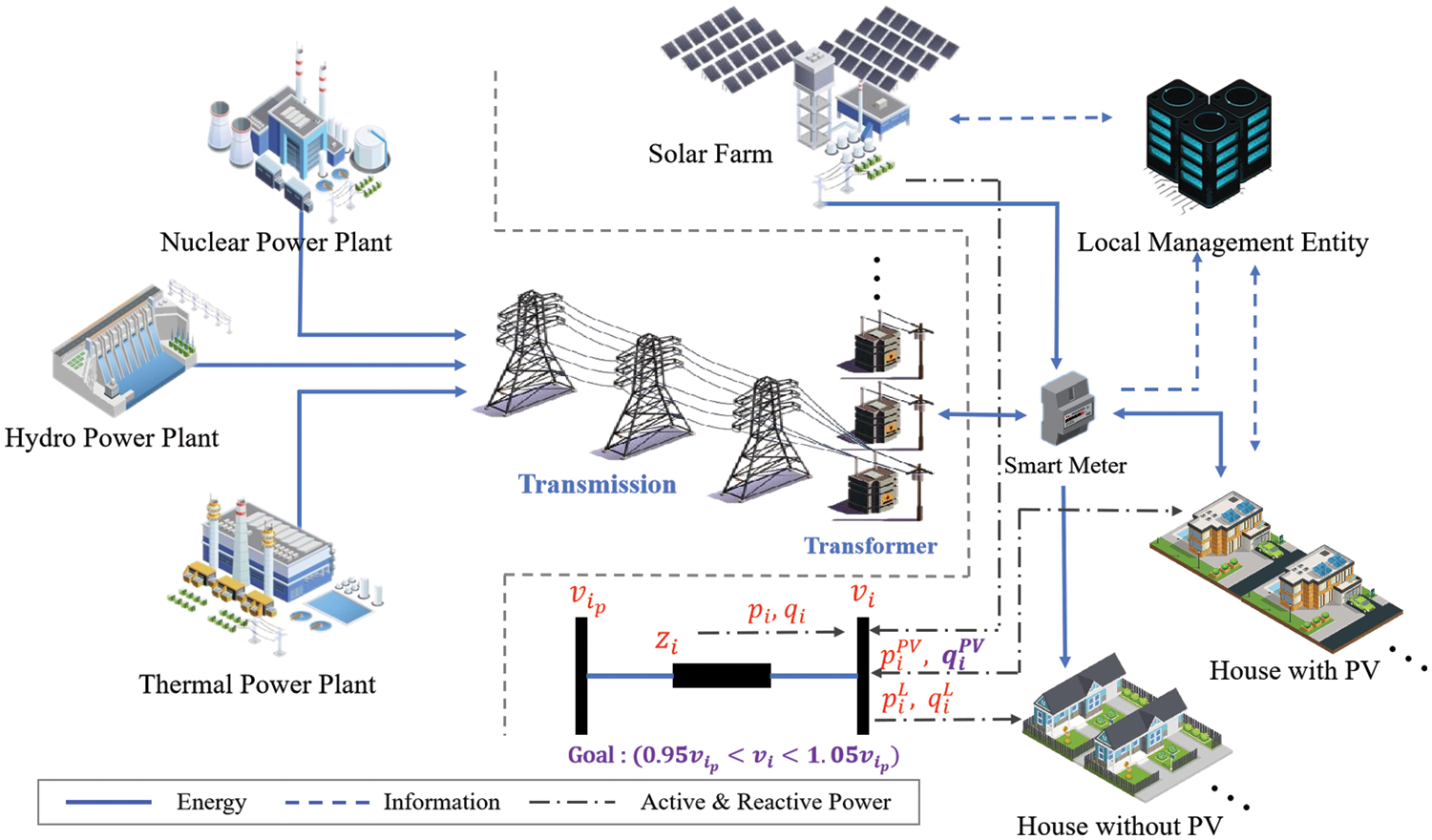
Figure 1: Illustration of distributed renewable energy networks

The power system dynamics can be defined as shown in Eqs. (1), (2), which is the cornerstone of solving the active power control and power flow problems [22].

piPV−piL=vi2∑j∈Ligij−vi∑j∈Livj(gijcosθij+bijsinθij),∀i∈L∖{0}(1)

qiPV−qiL=−vi2∑j∈Libij+vi∑j∈Livj(gijsinθij+bijcosθij),∀i∈L∖{0}(2)

In a distributed renewable energy network, it is assumed that there are L buses and N branches, where each bus i is associated with voltage value vi and phase angle θi. Power injection is represented by zi=pi+jqi. The set of buses connected to bus i is denoted as Li. The conductance and susceptance for bus i and j are denoted by gij and bij, respectively, while the phase difference between bus i and j is represented by θij=θi−θj. Active and reactive power at the PV nodes of bus i are denoted by piPV and qiPV, respectively. Active and reactive power consumed by the loads at bus i are represented by piL and qiL. To minimize the impact of voltage fluctuations on the grid, a safe range is defined as a 5% deviation from the baseline voltage. Assuming a baseline voltage of v0=1.0 at the grid side, denoted as unit (p.u.), the voltage at each bus must satisfy the condition outlined in (0.95p.u.≤vi≤1.05p.u.). During nighttime, when energy consumption and generation are relatively low, the voltage at corresponding buses may fall below (0.95p.u.). In contrast, during daytime with ample solar energy, the corresponding bus voltages may exceed (1.05p.u.), resulting in reverse power flow from the user side to the grid side [23].

To describe the voltage control relationship, we simplify the system into two buses. In Fig. 1, vip represents the voltage of a particular bus, which can be considered as the reference voltage. vi is the voltage of the bus connected to it, and the bus has loads and PV elements. The impedance between them is denoted as vi=ri+jxi, where ri is the resistance, and xi is the reactance. The voltage difference between these two buses is Δvi=vip−vi, as shown in Eq. (3).

Δvi=ri(piL−piPV)+xi(qiL−qiPV)vi(3)

The power loss is denoted as Ploss, as expressed in Eq. (4).

Ploss=(piL−piPV)2+(qiL−qiPV)2vip2⋅ri(4)

To minimize the voltage difference between the two buses, the control variable qiPV is adjusted to manipulate Δvi. Similarly, the adjustment of qiPV can also be employed to reduce power losses. It is crucial to note that, apart from qiPV, all other variables are uncontrollable.

3.2 Problem Formulation

The MARL approach to addressing multi-agent control problems is typically formulated as a Dec-POMDP, represented by a tuple (M,S,A,O,T,R,P,ρ,γ). The M denotes the set of agents. The S represents the set of states, describing the entire environment’s state. The A is the set of actions, with each element corresponding to the action of each individual agent. The O signifies the observable states for the agents, where each agent’s observed state may only capture a portion of the overall environment state. The T denotes the transition probabilities of the environment, describing the dynamic changes in the environment, with values ranging from [0,1]. The R is the set of rewards obtained by agents after executing actions in the environment. The P represents the observation function, indicating the probability of an agent observing a particular state after taking an action in a given state, with values in the range of [0,1]. The ρ is the probability distribution function for the initial state values, ranging from [0,1]. The γ is the discount factor, utilized to discount future rewards.

(1)   State and Observation Set:

In nodes within the bus, electrical data such as voltage, active power, and reactive power can be obtained through smart meters. In nodes equipped with PV systems, it is also necessary to monitor the active and reactive power of the PV system. The variables v and θ represent the voltage value and corresponding phase angle of the node’s bus, respectively, influenced by the power of the load and PV. The variables pL and qL represent the total active and reactive power of the load at the bus node, where the load generally consists of user electrical devices and is considered uncontrollable. The variables pPV and qPV represent the total active and reactive power of the PV system at the bus node. The system’s state can be represented as S={v,θ,pL,qL,pPV,qPV}. As each agent can only observe the state of its respective region, referred to as an observation, O signifies the measured voltage, active power, and reactive power within the region.

(2)   Action Set:

The overall bus voltage in the region is primarily influenced by the intermittent nature of PV generation, resulting in voltage instability. The main cause of this instability is the fluctuation in the active power generated by PV itself. To address this issue, voltage control can be achieved by adjusting the reactive power generated by the PV inverter. The adjustment of PV inverter reactive power can be expressed as qkPV=ak(skmax)2−(pkPV)2, where skmax represents the maximum apparent power for the corresponding bus node. The parameter ak represents the adjustment of the reactive power of the PV inverter, enabling the regulation of reactive power production and, consequently, the control of voltage on the corresponding bus. The range of ak is [−c, c], where the value of c is determined based on the load capacity.

(3)   Reward Function:

In the process of utilizing MARL for voltage control, the primary consideration is whether the post-operation voltage remains within a safe range. Subsequently, the objective is to minimize losses incurred by the production of reactive power. The reward function is defined as follows:

r=−α⋅lq(qPV)−1|V|∑i∈Vlv(vi)(5)

In the Eq. (5), lv represents the penalty function for voltage. Any deviation of the voltage from the designated standard voltage results in a corresponding penalty value calculated through the penalty function. The penalty is zero only when the voltage value aligns with the set standard voltage. a,b,c,d are set to 2, 0.095, 0.01, 0.04, respectively. lv is expressed as follows:

lv(vi)={a⋅|vi−vref|−bIf|vi−vref|>0.05−c⋅𝒩(vi|vref,0.1)+dOtherwise(6)

lq is computed to quantify the loss due to the production of reactive power, denoted as:

lq(qPV)=1|M|‖qPV‖1(7)

The α denotes the proportion of reactive power generation loss, ranging from [0,1].

The objective is to maximize the reward, denoted as maxπ⁡Eπ[∑t=0∞γtrt], with π representing the policy of the agent.

3.3 Multi-Agent Reinforcement Learning

In comparison to single-agent reinforcement learning, the environment in which multiple agents operate is more intricate. In collaborative tasks, each intelligent agent is tasked not only with maximizing its individual rewards but also with considering the collective achievement of goals with other agents. However, each agent, in the process of exploration, observes only a partial aspect of the environment, rendering each trained agent highly unstable. To address this issue, the concept of centralized training with decentralized execution has been proposed [24]. During the training phase, each agent explores the environment and collects transitions, which are then uniformly stored in a replay buffer. Once transitions from all agents are gathered, a critic network is trained using all the data. The policy network of each agent is trained locally based on the Q values provided by the critic. Consequently, upon completion of training, the agents can execute tasks locally.

In reinforcement learning algorithms, the issue of overestimation often arises in value estimation networks, impeding the convergence of the reinforcement learning algorithm. To address this problem, approaches such as DDQN [25], Dueling DQN [26], and TD3 [27] have been successively proposed. Among these, TD3 has demonstrated effective mitigation of issues arising from overestimation. TD3 employs a dual actor-critic network structure, comprising a main network and a target network. The critic utilizes two networks to estimate Q values and selects the minimum value for updating the policy network. To further alleviate overestimation issues, the Actor is updated with a delay after several steps of critic training, ensuring more stable convergence. The MATD3 algorithm integrates the CTDE-derived algorithm into the TD3 framework and is designed to address challenges in multi-agent environments. The algorithmic framework of MATD3 is illustrated in Fig. 2.

Figure 2: The algorithmic framework of MATD3

In the context of agent, the policy network of the main actor in agent is represented as μ(oi;θiμ), with hyperparameters θiπ, and the input is the observation currently perceived by the agent within the region. The output of the policy network, denoted as ai, represents the reactive power adjustment of each PV inverter. There are two critics, Q1 and Q2, with hyperparameters θiQ1 and θiQ2, respectively. After the actor outputs ai, Q1 and Q2 take the observations of all agents within the region at the same time and ai as inputs to calculate the Q values. The minimum Q value is then used to update the critic networks. The target networks are not trained; their hyperparameters are periodically updated from the main network. The hyperparameters of the target actor are denoted as θ¯iμ, and those of the two target critics are denoted as θ¯iQ1 and θ¯iQ2. The hyperparameter update is determined by the soft update parameter β as shown in Eqs. (8)–(10).

θ¯iμ=βθiμ+(1−β)θ¯iμ(8)

θ¯iQ1=βθiQ1+(1−β)θ¯iQ1(9)

θ¯iQ2=βθiQ2+(1−β)θ¯iQ2(10)

To prevent the overestimation problem of the critics, the minimum Q value is selected for updating the networks. The critic networks of the main network are updated using the Q values from the target networks. The objective of training the main network is to make the output Q values as close as possible to the values of the target network plus the reward obtained from environmental exploration, as shown in Eq. (11).

yit+γ⋅min(Qj(o1t+1,…,oNt+1,a~1t+1,…,a~Nt+1;θ¯iQj));j=1,2(11)

where γ is the discount factor, a~it+1 is the target output action, and Gaussian noise with clipping is added as shown in Eq. (12).

a~it+1=π(oi;θiμ)+clip(𝒩(0,σ),−ci,ci)(12)

𝒩(0,σ) is random noise following a standard Gaussian distribution, and ci defines the maximum and minimum values of the noise. After obtaining the minimum Q value from the output of the target critic networks, denoted as y, the main critic networks are updated using the loss function represented in Eqs. (13), (14).

J(θiQ1)=Eot,at,rt,ot+1[(Q1(o1t,…,oNt,a1t,…,aNt;θiQ1)−yit)2](13)

J(θiQ2)=Eot,at,rt,ot+1[(Q2(o1t,…,oNt,a1t,…,aNt;θiQ2)−yit)2](14)

After calculating the loss values for the two target networks, the network parameters θiQ1 and θiQ2 are updated through backpropagation, as shown in Eqs. (15), (16).

θiQ1=θiQ1−α∇θiQ1J(θiQ1)(15)

θiQ2=θiQ2−α∇θiQ2J(θiQ2)(16)

The α is the learning rates for the two main critic networks. The update of the main actor is based on the Q values output by the two main critic networks, and the loss function is represented as shown in Eq. (17).

∇θiμJ(θiμ)=Eot,at[∇θiμμi(oit;θiμ)∇aiQ(o1t,…,oNt,a1t,…,aNt;θiQ)|ai=μi(oit;θiμ)(17)

After obtaining the loss through Q values, the hyperparameters of the main actor network are updated through backpropagation, as shown in Eq. (18).

θiμ=θiμ−α∇θiμJ(θiμ)(18)

The α is the learning rate of the main actor network.

3.4 Safety-Constrained MARL for Power Quality Control

In the context of distributed renewable energy networks, each embedded node with PV is considered as an agent. Each agent explores the environment, collecting observed observations, and takes corresponding actions. However, due to the lack of prior knowledge during the initial training of agents, actions taken by the agents may cause voltage to exceed the safe range, posing unknown potential risks. To ensure that agents make safe actions, we propose imposing safety constraints on their actions before execution. After an agent takes an action, the output action is subjected to a safety check within the safety constraint module. In this module, the input consists of observed observations by the agent, including the voltage value v. It is imperative to assess whether the voltage falls within the safe range, defined as [0.95 + η, 1.05 − η], where η is set to 0.025 in the paper, signifying a narrowed voltage safety range of [0.975,1.025]. This adjustment aims to enhance the algorithm’s fault-tolerance space. When the voltage exceeds the designated safety range, a quadratic programming (QP) is solved to determine the corrective action that satisfies safety conditions. The calculated corrective action is then fed back to the agent to adjust its output action, which is subsequently utilized for training the policy network. If the voltage remains within the established safe range, no further action is taken, as illustrated in Fig. 3.

Figure 3: The diagram of safety-constrained MARL for power quality control

In a specific region, the action of each agent influences the voltage at various bus points to varying degrees. This means that changes in bus voltage can be attributed to two main factors: Inherent characteristics of the bus and the actions of other agents. Therefore, when bus voltages exceed the predefined safety range, it is essential to accurately assess the impact of each action on all bus voltages. To achieve this, we must calculate the partial derivatives of the voltage at each bus with respect to the actions of all agents. This approach allows for a more precise understanding of how individual actions affect the overall voltage stability in the region. This is represented using the Jacobian matrix, as shown in Eq. (19).

∇atvt=[∂v1t∂a1t⋯∂v1t∂ant⋮⋱⋮∂vmt∂a1t⋯∂vmt∂ant]m×n(19)

The variable m represents the number of buses, N denotes the number of agents, and the overall nodal voltage of the system, excluding the embedded PV inverter, is influenced by the actions performed by agents. The t signifies the current time step, and t+1 represents the subsequent time step. The a1t represents the action executed by the i-th agent at time t. According to the Taylor series expansion, if a small change Δat is added to at, the expression for the voltage at the next time step t+1 can be formulated as follows Eq. (20).

vt+1=vt+∇atvtΔat(20)

To guarantee that the voltage determined from solving Eq. (20) adheres to the specified safety constraints, we have reformulated the problem. It is now presented as the solution to a Quadratic Programming (QP) problem, which is detailed in Eq. (21).

minΔat12‖ Δat ‖2,s.t.{ vt+∇atvtΔat≤1.05−ηvt+∇atvtΔat≥0.95−η(21)

The boundary value for the safety range, denoted as η>0, is set to 0.025, as the voltage must not exceed the safety range during the MARL process. Building upon this constraint, we further limit it to ensure safety during the training phase of MARL. By solving a quadratic programming problem, we obtain the optimal correction term Δat. Consequently, when the total bus voltage within the region exceeds the predefined safety range, the action taken by the agent, in addition to the correction term Δat, facilitates the return of the voltage to the safety range. Consequently, the safety constraint module ensures that MARL maintains control of the voltage within the safety range throughout both the training and testing phases.

4  Experiments

4.1 Experiment Setups

To validate the proposed SC-MARL for power quality control, we employed the open-source distributed power grid environment MAPDN [2] as our simulation platform. To demonstrate the robust performance of SC-MARL across power grids of varying scales, three distributed power grids of different sizes were utilized, namely, 33-buses, 141-buses, and 322-buses. The data used consisted of three years of records at 3-min intervals, with 2 years allocated for training and 1 year for validating the performance of different algorithms. Five commonly used MARL algorithms were selected for comparison with SC-MARL in the experiments. The performance of the proposed method was contrasted with that of other algorithms. To assess and compare the performance of SC-MARL and other algorithms, five distinct evaluation metrics were employed, allowing for a comprehensive analysis from various perspectives. Finally, for visual representation of the control efficacy of voltage, we chose a specific day in summer and winter for the 33-buses, 141-buses, and 322-buses, employing visualization techniques in the experiments.

4.1.1 Distributed Renewable Power Network

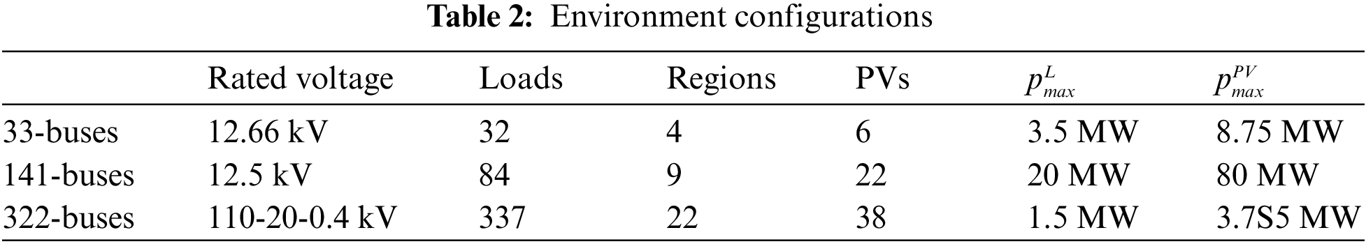
In the experiment, three different scales of power grids were employed, namely, 33-buses, 141-buses, and 322-buses. Their voltage levels were 12.66 kV, 12.5 kV, and 110-20-0.4 kV, respectively. The 322-buses scale is comparatively large, and to emphasize flexibility and diversity, three different voltage levels were utilized for assessing the performance of MARL across varying voltage networks. The power grids were equipped with varying numbers of loads and PVs, with load quantities of 32, 84, and 337, and PV quantities of 6, 22, and 38, respectively. Each power grid was partitioned into distinct regions, with the numbers of regions being 4, 9, and 22 for 33-buses, 141-buses, and 322-buses, respectively. The maximum active power of loads and PVs for the 33-buses system were 3.5 and 8.75 MW, respectively. For the 141-buses system, the maximum active power of loads and PVs were significantly larger at 20 and 80 MW, providing a basis for comparing the performance of MARL in networks with different active power levels. The 322-buses system had a maximum active power of 1.5 MW for loads and 3.75 MW for PVs. The distributed renewable energy environment configurations are presented in the Table 2.

The size of the figure is measured in centimeters and inches. Please adjust your figures to a size within 17 cm (6.70 in) in width and 20 cm (7.87 in) in height. Figures should be in the original scale, with no stretch or distortion. The network structure of the 33-buses system is illustrated in Fig. 4. We have partitioned the network into four zones, each characterized by varying quantities of loads and PV sources. Bus 0 typically serves as the bus interfacing with the main power grid. In zones 2 and 3, there is a single PV source connected to bus 1 and 2. Conversely, zones 1 and 4 feature two PV sources each, connected to bus 5. Within a given zone, each agent, which is linked to the bus where the photovoltaic (PV) source is situated, has the ability to monitor the voltage and power levels of other buses in the same zone. However, this capability to observe does not extend to buses located in different zones.

Figure 4: The network structure of the 33-buses system

4.1.2 Data Descriptions

The load data was collected in real-time from the electricity consumption of 232 power users in the Portuguese region over a period of three years [28]. The original dataset comprised electricity consumption readings at 15-min intervals for a total of 370 residential and industrial entities spanning the years 2012 to 2015. Data collection commenced on January 01, 2012, at 00:15:00. Due to the presence of some missing values, a subset of users was excluded, resulting in a final dataset consisting of 232 power users. To enhance the temporal resolution, the data was imputed to transform the 15-min intervals into 3-min intervals. The ultimate dataset dimensions were 526,080 × 232, covering 232 users over a span of 1,096 days.

Given that 322 buses were required, and to address the shortfall in users, load data was randomly duplicated from the existing 232 users to compensate for the missing data in the 322 buses. Additionally, Gaussian random noise was introduced to the duplicated data. PV data was sourced from the Elia group [28], with a resolution of 3 min and a total dataset size of 526,080 × 232. For the 33-bus configuration, encompassing 4 regions, the available PV profiles were deemed sufficient. In the case of the 141-bus configuration, featuring 9 regions, the PV data was utilized. Concerning the 322-bus configuration, comprising 22 regions, PV data for the 22 regions was obtained through random duplication, followed by the introduction of Gaussian random noise.

The load and PV power profiles for bus 13, 18, and 23 of the 33-buses system during winter and summer are depicted in Fig. 5. For bus-13, the disparity between winter and summer load powers is marginal, as consumer electricity demand exhibits relatively limited variation. However, there is a substantial difference in PV power, primarily attributed to abundant sunlight during the summer, resulting in approximately a twofold increase in PV generation compared to winter. Bus 18 exhibits similarities to bus 13, with the distinction that power consumption during winter is higher than in summer. In the case of bus 23, PV generation is lower during winter, while in summer, the PV output is approximately four times that of winter.

Figure 5: Daily power of 33-buses network of winter (January, 1st raw) and summer (July, 2nd raw). The (a), (b) and (c) are bus 13, bus 18 and bus 23, respectively

The load and PV power profiles for bus 36, 111, and 53 of the 141-buses system during both winter and summer seasons are illustrated in Fig. 6. It is noteworthy that bus 53 exhibits substantial PV generation in both winter and summer, with increased sunlight availability during the summer season. However, the load power is relatively small. Consequently, the injection of a significant amount of active power from PV sources into the bus can result in voltage fluctuations, leading to grid disturbances. In such scenarios, it becomes imperative to regulate the PV inverters, inducing them to generate reactive power to absorb the surplus active power. This action aims to stabilize the bus voltage, ensuring overall grid safety and reliability.

Figure 6: Daily power of 141-buses network of winter (January, 1st raw) and summer (July, 2nd raw). The (a), (b) and (c) are bus 36, bus 111 and bus 53, respectively

The load and PV power curves for bus 70, 111, and 53 of the 322-buses system during both winter and summer seasons are illustrated in Fig. 7. In the summer, the scenario is analogous to that of the 33-buses system in winter. Conversely, during the winter, the PV generation power of the 322-buses system is extremely low. Owing to the presence of a significant number of inverters on the PV, power is consumed on the bus, resulting in bus voltage falling below the lower limit of the safety range and causing grid instability. To address this issue, the impact of PV inverters on the grid is mitigated by controlling the reactive power of the PV inverters. In summary, weak sunlight during the winter results in lower PV generation power, leading to voltages below the lower limit of the safety range. Conversely, strong sunlight during the summer results in higher PV generation power, causing voltages to exceed the upper limit of the safety range.

Figure 7: Daily power of 322-buses network of winter (January, 1st raw) and summer (July, 2nd raw). The (a), (b) and (c) are bus 70, bus 74 and bus 132, respectively

4.1.3 MADRL Algorithm Settings

In the experiment, we selected five commonly used MARL algorithms for performance comparison with our proposed model. These algorithms are MATD3, MAPPO [29], MADDPG, IPPO [30], and COMA [31]. SC-MARL is an extension of MATD3 with the addition of a safety constraint module. To assess their performance, all algorithms were trained for a total of 400 episodes, with each episode consisting of 480 steps, corresponding to one day (3-min intervals). Due to variations in training methodologies, the training was conducted using both online and offline approaches. IPPO, COMA, and MAPPO were trained online, with the network being updated after each episode. On the other hand, MATD3 and MADDPG were trained offline, with policy network updates occurring after each episode as well. The learning rate was set to 0.0001, and the L1 norm clip bound was set to 1. The batch size was fixed at 32. For offline algorithms, the replay buffer size was set to 5000. Notably, COMA had a sample size of 10 for its replay buffer. Additionally, IPPO and MAPPO had a value loss coefficient of 2, with a clip bound of 0.4.

4.1.4 Evaluation Metrics

To evaluate the performance of the proposed SC-MARL model in comparison to other MARL models, five metrics were employed in the experiments, namely controllable rate, average reward, reactive power loss, average voltage, and voltage out of control rate.

(1) Controllable Rate (%CR): It is calculated as the proportion of all buses controlled at each time step in every episode. Specifically, it represents the ratio of the number of times the controller has taken control over a period of time to the total number of time steps. The controllable rate ranges from 0 to 1, with a higher value indicating better performance.

(2) Average Reward (Avr.R): It measures the average sum of rewards obtained by all agents at each time step within each episode. The average reward falls within the range of [−8, 0], and a value closer to 0 is indicative of better performance.

(3) Reactive Power Loss (Q loss): It represents the average reactive power loss generated by all agents at each time step in every episode. The reactive power loss metric also ranges from [−8, 0].

(4) Average Voltage (V.pu): It calculates the average voltage at each time step for all buses within each episode. The average voltage is around 1, and a value closer to 1 is considered desirable.

(5) Voltage Out of Control Rate (%V.out): It is the average proportion of time steps in which the voltage of any bus goes out of control during each episode. The voltage out of control rate ranges from [0,1], and a lower value indicates better control performance.

4.2 Results

In voltage control, voltage fluctuations occur frequently. To prevent the voltage from exceeding the predetermined safety range, it is essential for the controller to perform real-time processing of voltage fluctuations rather than waiting until the voltage is close to the dangerous threshold to react. The controllable rate is employed to measure the real-time control proportion of the controller. A comparative analysis of the controllable rates for COMA, IPPO, MADDPG, MATD3, MAPPO, and SC-MARL is presented in Fig. 8 across 33-buses, 141-buses, and 322-buses scenarios. SC-MARL demonstrates outstanding performance across different buses. However, there is some notable fluctuation in the 322-buses scenario, primarily attributed to the large network scale, with certain bus nodes stabilizing and requiring minimal intervention.

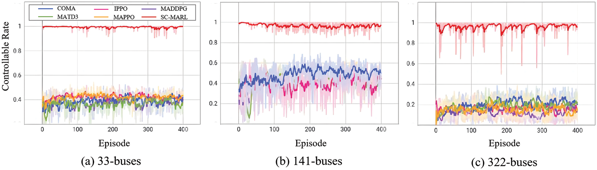
Figure 8: The comparative analysis of the controllable rate. The (a), (b) and (c) are 33-buses, 141-buses and 322-buses, respectively

In the process of exploration, the agent, lacking any prior knowledge during the early stages of training, initially experiences lower rewards. A comparative analysis of Average Rewards for COMA, IPPO, MADDPG, MATD3, MAPPO, and SC-MARL is presented in Fig. 9 across 33-buses, 141-buses, and 322-buses scenarios. As the agent continues to explore and learn, it gradually tends to favor actions that result in greater rewards. The inclusion of a safety constraint in our algorithm significantly reduces the margin for agent errors. Consequently, the agent learns safe actions from the outset, leading to higher rewards. In comparison to other algorithms, the proposed algorithm exhibits characteristics such as rapid convergence and high safety, making it more suitable for scenarios where safety is a primary concern.

Figure 9: The comparative analysis of the average reward. The (a), (b) and (c) are 33-buses, 141-buses and 322-buses, respectively

The primary objective of voltage control is to regulate voltage by controlling the generation of reactive power. The generation of reactive power results in power wastage; therefore, concurrently with voltage control, minimizing the generation of reactive power is also crucial. We compared the Reactive Power Loss of COMA, IPPO, MADDPG, MATD3, MAPPO, and SC-MARL in a 33-buses, 141-buses, and 322-buses system, as illustrated in Fig. 10. The proposed SC-MARL, when employed for voltage control, consistently exhibits lower levels of generated reactive power compared to other algorithms. As the number of episodes increases, the agent gradually reduces the generation of reactive power. The objective is to control voltage within a safe range while minimizing the production of reactive power as much as possible.

Figure 10: The comparative analysis of the reactive power loss. The (a), (b) and (c) are 33-buses, 141-buses and 322-buses, respectively

Maintaining voltage within a safe range and ensuring stability are critical aspects of control. We compared the Average Voltage of COMA, IPPO, MADDPG, MATD3, MAPPO, and SC-MARL across 33-buses, 141-buses, and 322-buses scenarios, as depicted in Fig. 11. In contrast to other algorithms, SC-MARL exhibits comparatively stable voltage control with minimal fluctuations. In the case of the 141-buses scenario, MADDPG and MATD3 demonstrate significant voltage fluctuations, exceeding the safe range early in the training phase an undesirable occurrence. Within the 322-buses scenario, MAPPO also exceeds the safe range in the initial stages of training and exhibits substantial fluctuations throughout the training process. Although SC-MARL does not precisely maintain voltage around 1, it underscores that the pivotal control objective is the safety and stability of the voltage rather than a specific numerical target.

Figure 11: The comparative analysis of the average voltage. The (a), (b) and (c) are 33-buses, 141-buses and 322-buses, respectively

Once the voltage exceeds the designated safety range, the stability of the power grid cannot be guaranteed, making voltage control a pivotal concern. We conducted a comparative analysis of the Average Voltage for COMA, IPPO, MADDPG, MATD3, MAPPO, and SC-MARL across 33-buses, 141-buses, and 322-buses systems, as depicted in Fig. 12. Due to the incorporation of safety constraints, SC-MARL exhibits minimal instances of voltage instability, even during the early stages of training. In the case of the 141-buses system, lacking prior knowledge in the initial training phase results in MATD3 experiencing an alarming 80% rate of voltage instability, posing a potentially fatal threat to the power grid. Similarly, in the 322-buses system, MAPPO exhibits high levels of instability, reaching 50% during the early stages of training. Although the voltage instability diminishes with continuous training, deploying these models in practical scenarios may expose them to potential control risks.

Figure 12: The comparative analysis of the voltage out of control rate. The (a), (b) and (c) are 33-buses, 141-buses and 322-buses, respectively

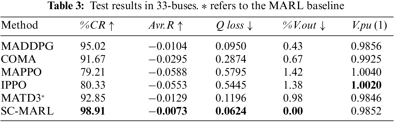
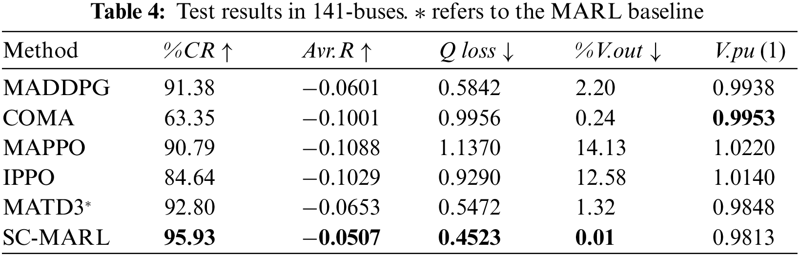
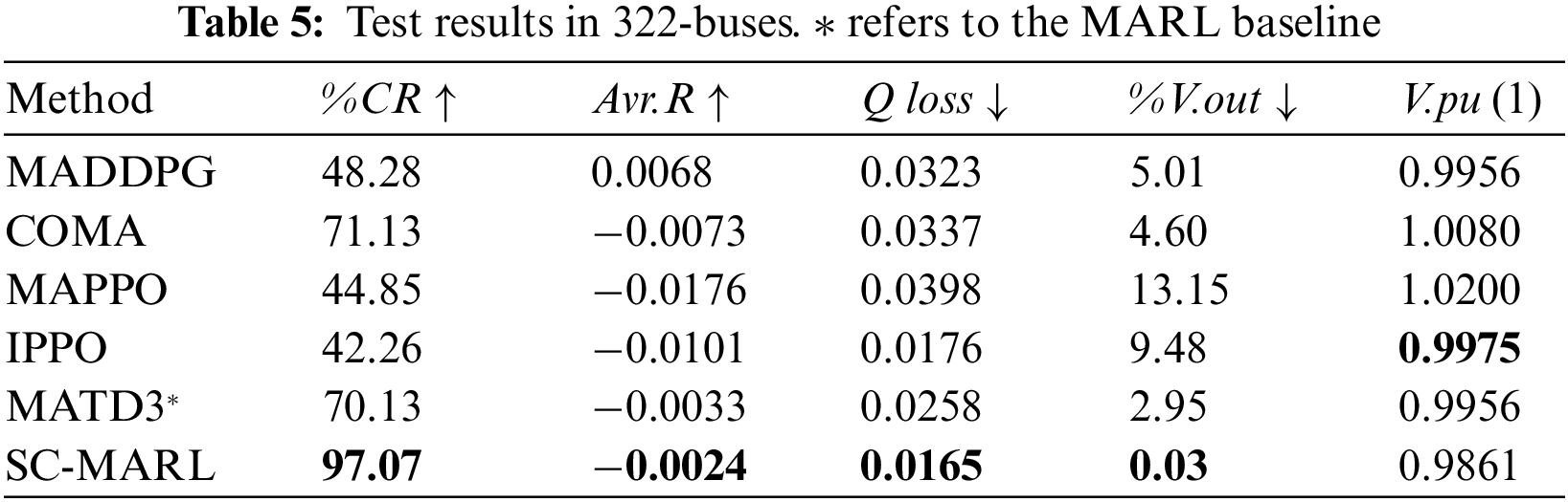
To assess the performance of the proposed algorithm, we randomly selected 10 episodes from the test sets of 33-buses, 141-buses, and 322-buses scenarios and conducted evaluations on the COMA, IPPO, MADDPG, MATD3, MAPPO, and SC-MARL algorithms. The test results are presented in Tables 3–5. It is noteworthy that the %V.out metric of SC-MARL is significantly lower than that of other algorithms, particularly evident in the 33-bus scenario where the proportion of voltage exceeding the safety range is zero. This demonstrates the algorithm’s robust safety profile. Additionally, SC-MARL outperforms other algorithms in terms of control proportion, notably in the 322-bus scenario where it surpasses all others, maintaining a high control ratio even in large-scale power grids. One limitation is that the voltage value cannot be adjusted to stabilize around 1 due to our set value of η as 0.025; hence, SC-MARL controls the voltage to approximately 0.98. In summary, our proposed SC-MARL demonstrates the capability to safely and stably control voltage while minimizing reactive power generation as much as possible, both during training and testing phases.

In the context of 33-buses, 141-buses, and 322-buses power systems, a comparative analysis was conducted for a selected day in winter (January) and summer (July), with a time interval of 3 min. Three scenarios were considered: No control (None), utilization of the optimal MARL algorithm, and application of SC-MARL for voltage control. The results are illustrated in Fig. 13. During summer in the 33-buses system, the high reactive power output from PV sources resulted in voltages exceeding the upper limit of the safety range between 190 and 310. MARL was unable to consistently maintain voltages within the safe range at every time point, whereas SC-MARL exhibited superior and stable control, ensuring safety. In the case of the 141-buses and 322-buses systems, SC-MARL consistently demonstrated excellent control performance, ensuring both the safety and stability of voltages within the specified ranges.

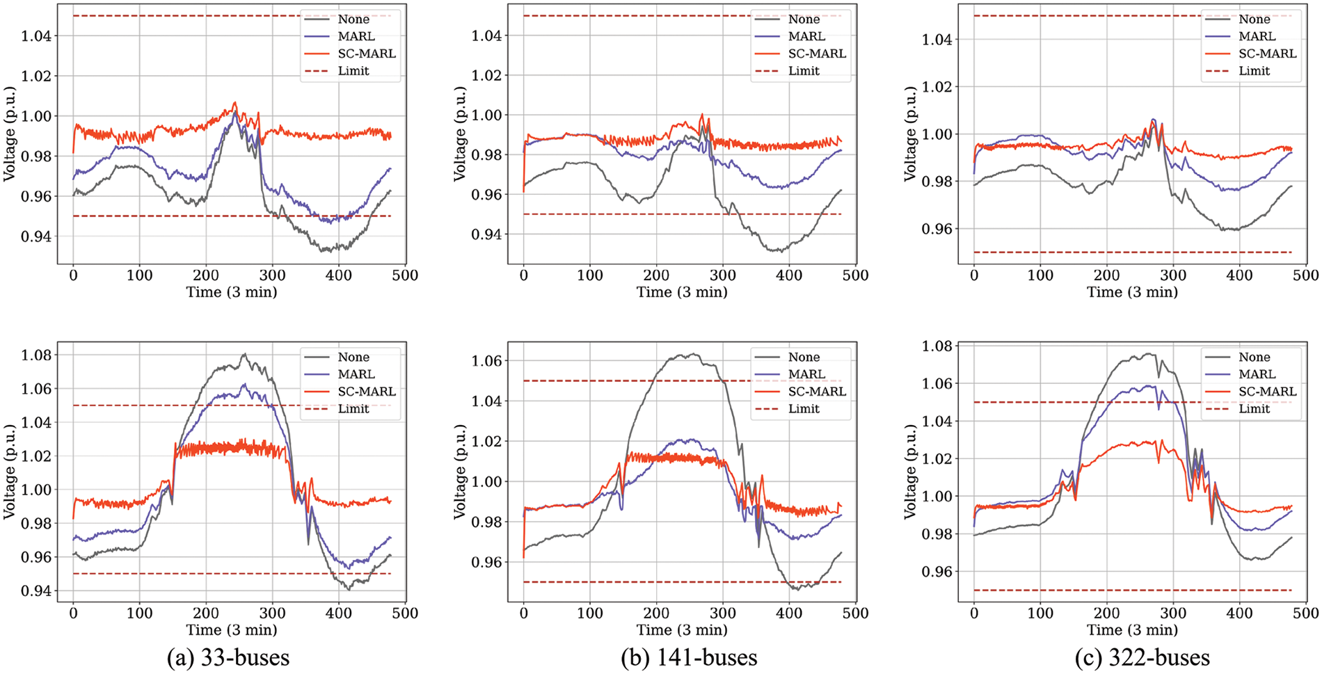
Figure 13: The curves of voltage control. The (a), (b) and (c) are 33-buses, 141-buses and 322-buses, respectively

5  Conclusion

This paper introduces a Safety-Constrained Multi-Agent Reinforcement Learning (SC-MARL) approach for power quality control. We have conducted experiments where the SC-MARL algorithm was trained and benchmarked against five other Multi-Agent Reinforcement Learning (MARL) algorithms using five key performance metrics. The results from our tests show that the SC-MARL algorithm effectively manages voltage control in power systems with 33, 141, and 322 buses. In the 33-buses system, specifically, the Controllable Rate (%CR) increased from 95.02% to 98.91%, the Average Reward (Avr.R) increased from −0.0104 to −0.0073, the Reactive Power Loss (Q loss) decreased from 0.095 to 0.0624, and the Average Voltage (V.pu) was 0.9852. Additionally, the Voltage Out of Control Rate (%V.out) decreased from 0.43 to 0. Notably, the percentage of voltage surpassing the safety range was almost zero during both the training and testing phases. This robust voltage control underscores the potential of SC-MARL for practical deployment in power grids.

A noted limitation of our experiment is that due to the safety constraint module, which specifies a voltage safety range of [0.975,1.025], the SC-MARL tends to maintain the voltage around 0.98. Although this does not present immediate concerns, it does highlight an area for further research.

In conclusion, SC-MARL demonstrates effective and safe voltage control capabilities, crucial as the integration of photovoltaic systems into power grids escalates. This ensures high-quality electrical energy and minimizes energy losses. Future research will aim to refine the safety strategies of SC-MARL, enhancing its practical application in real-world power grid scenarios.

Acknowledgement: We would like to express our sincere gratitude to the Regional Innovation Strategy (RIS) for their generous support of this research. This work was made possible through funding provided by the National Research Foundation of Korea (NRF) under the Ministry of Education (MOE), Grant Number 2021RIS-002. We appreciate the opportunity to conduct this study and acknowledge the invaluable assistance provided by the NRF and MOE in advancing our research endeavors. Their support is instrumental in driving innovation and contributing to the advancement of knowledge in our field.

Funding Statement: This research was supported by “Regional Innovation Strategy (RIS)” through the National Research Foundation of Korea (NRF) funded by the Ministry of Education (MOE) (2021RIS-002).

Author Contributions: The authors confirm contribution to the paper as follows: Study conception and design: Y. Zhao, H. Zhong; data collection: Y. Zhao, H. Zhong; analysis and interpretation of results: Y. Zhao; draft manuscript preparation: Y. Zhao; C. Lim reviewed the results and approved the final version of the manuscript.

Availability of Data and Materials: Data openly available in a public repository. The data that support the findings of this study are openly available in MAPDN at https://drive.google.com/file/d/1-GGPBSolVjX1HseJVblNY3KoTqfblmLh/view?usp=sharing.

Conflicts of Interest: The authors declare that they have no conflicts of interest to report regarding the present study.

References

1. H. Yeh, D. F. Gayme, and S. H. Low, “Adaptive VAR control for distribution circuits with photovoltaic generators,” IEEE Trans. Power Syst., vol. 27, no. 3, pp. 1656–1663, 2012. doi: 10.1109/TPWRS.2012.2183151. [Google Scholar] [CrossRef]

2. D. Hu, Z. Ye, Y. Gao, Z. Ye, Y. Peng and N. Yu, “Multi-agent deep reinforcement learning for voltage control with coordinated active and reactive power optimization,” IEEE Trans. Smart Grid, vol. 13, no. 6, pp. 4873–4886, 2022. doi: 10.1109/TSG.2022.3185975. [Google Scholar] [CrossRef]

3. E. Batzelis et al., “Solar integration in the UK and India: Technical barriers and future directions,” in JUICE White Paper on Solar Integration, 2021. doi: 10.17028/rd.lboro.14453133.v1. [Google Scholar] [CrossRef]

4. Y. P. Agalgaonkar, B. C. Pal, and R. A. Jabr, “Distribution voltage control considering the impact of PV generation on tap changers and autonomous regulators,” IEEE Trans. Power Syst., vol. 29, no. 1, pp. 182–192, 2014. doi: 10.1109/TPWRS.2013.2279721. [Google Scholar] [CrossRef]

5. L. H. Wu, F. Zhuo, P. B. Zhang, H. Y. Li, and Z. A. Wang, “Study on the influence of supply-voltage fluctuation on shunt active power filter,” IEEE Trans. Power Deliv., vol. 22, no. 3, pp. 1743–1749, 2007. doi: 10.1109/TPWRD.2007.899786. [Google Scholar] [CrossRef]

6. D. Cao et al., “Reinforcement learning and its applications in modern power and energy systems: A review,” J. Mod. Power Syst. Clean Energy, vol. 8, no. 6, pp. 1029–1042, 2020. doi: 10.35833/MPCE.2020.000552. [Google Scholar] [CrossRef]

7. Y. Wang, D. Qiu, G. Strbac, and Z. Gao, “Coordinated electric vehicle active and reactive power control for active distribution networks,” IEEE Trans. Industr. Inf., vol. 19, no. 2, pp. 1611–1622, 2023. doi: 10.1109/TII.2022.3169975. [Google Scholar] [CrossRef]

8. D. Cao, W. Hu, J. Zhao, Q. Huang, Z. Chen and F. Blaabjerg, “A multi-agent deep reinforcement learning based voltage regulation using coordinated PV inverters,” IEEE Trans. Power Syst., vol. 35, no. 5, pp. 4120–4123, 2020. doi: 10.1109/TPWRS.2020.3000652. [Google Scholar] [CrossRef]

9. B. Zhang, A. M. Y. M. Ghias, and Z. Chen, “A multi-agent deep reinforcement learning based voltage control on power distribution networks,” in 2022 IEEE PES Innov. Smart Grid Technol.—Asia (ISGT Asia), Singapore, 2022, pp. 761–765. [Google Scholar]

10. H. Liu and W. Wu, “Online multi-agent reinforcement learning for decentralized inverter-based Volt-VAR control,” IEEE Trans. Smart Grid, vol. 12, no. 4, pp. 2980–2990, 2021. doi: 10.1109/TSG.2021.3060027. [Google Scholar] [CrossRef]

11. T. Senjyu, Y. Miyazato, A. Yona, N. Urasaki, and T. Funabashi, “Optimal distribution voltage control and coordination with distributed generation,” IEEE Trans. Power Deliv., vol. 23, no. 2, pp. 1236–1242, 2008. doi: 10.1109/TPWRD.2007.908816. [Google Scholar] [CrossRef]

12. G. Fusco and M. Russo, “A decentralized approach for voltage control by multiple distributed energy resources,” IEEE Trans. Smart Grid, vol. 12, no. 4, pp. 3115–3127, 2021. doi: 10.1109/TSG.2021.3057546. [Google Scholar] [CrossRef]

13. E. D. Anese, S. V. Dhople, and G. B. Giannakis, “Optimal dispatch of photovoltaic inverters in residential distribution systems,” in 2014 IEEE PES Gen. Meet.|Conf. Expos., National Harbor, MD, USA, 2014. [Google Scholar]

14. W. Zheng, W. Wu, B. Zhang, H. Sun, and Y. Liu, “A fully distributed reactive power optimization and control method for active distribution networks,” IEEE Trans. Smart Grid, vol. 7, no. 2, pp. 1021–1033, Mar. 2016. [Google Scholar]

15. A. Singhal, V. Ajjarapu, J. Fuller, and J. Hansen, “Real-time local volt/var control under external disturbances with high PV penetration,” IEEE Trans. Smart Grid, vol. 10, no. 4, pp. 3849–3859, 2019. doi: 10.1109/TSG.2018.2840965. [Google Scholar] [CrossRef]

16. M. Zeraati, M. E. H. Golshan, and J. M. Guerrero, “Voltage quality improvement in low voltage distribution networks using reactive power capability of single-phase PV inverters,” IEEE Trans. Smart Grid, vol. 10, no. 5, pp. 5057–5065, 2019. doi: 10.1109/TSG.2018.2874381. [Google Scholar] [CrossRef]

17. D. Cao et al., “Data-driven multi-agent deep reinforcement learning for distribution system decentralized voltage control with high penetration of PVs,” IEEE Trans. Smart Grid, vol. 12, no. 5, pp. 4137–4150, 2021. doi: 10.1109/TSG.2021.3072251. [Google Scholar] [CrossRef]

18. K. H. Wray and S. Zilberstein, “Generalized controllers in POMDP decision-making,” in 2019 Int. Conf. Robot. Autom. (ICRA), Montreal, QC, Canada, 2019, pp. 7166–7172. [Google Scholar]

19. P. Chen and C. Kuo, “Bi-objective hydroelectric optimal dispatch under electricity deregulated environment,” in 2005 IEEE/PES Transm. Distrib. Conf. Expo., Asia and Pacific, Dalian, China, 2005, pp. 1–5. [Google Scholar]

20. F. J. G. Polo and F. F. Rebollo, “Safe reinforcement learning in high-risk tasks through policy improvement,” in 2011 IEEE Symp. Adapt. Dyn. Program. Reinf. Learn. (ADPRL), Paris, France, 2011, pp. 76–83. [Google Scholar]

21. W. Meng, Q. Zheng, Y. Shi, and G. Pan, “An off-policy trust region policy optimization method with monotonic improvement guarantee for deep reinforcement learning,” IEEE Trans. Neural Netw. Learn. Syst., vol. 33, no. 5, pp. 2223–2235, 2022. doi: 10.1109/TNNLS.2020.3044196 [Google Scholar] [PubMed] [CrossRef]

22. S. Chiniforoosh et al., “Definitions and applications of dynamic average models for analysis of power systems,” IEEE Trans. Power Deliv., vol. 25, no. 4, pp. 2655–2669, 2010. doi: 10.1109/TPWRD.2010.2043859. [Google Scholar] [CrossRef]

23. Y. P. Agalgaonkar, B. C. Pal, and R. A. Jabr, “Multi-agent actor-critic for mixed cooperative-competitive environments,” IEEE Trans. Power Syst., vol. 29, no. 1, pp. 182–192, 2014. doi: 10.1109/TPWRS.2013.2279721. [Google Scholar] [CrossRef]

24. R. Lowe, Y. Wu, A. Tamar, J. Harb, P. Abbeel and I. Moedatch, “Multi-agent actor-critic for mixed cooperative-competitive environments,” in Adv. Neural Inf. Process. Syst., Long Beach, CA, USA, 2017, pp. 6379–6390. [Google Scholar]

25. H. Hasselt, A. Guez, and D. Silver, “Deep reinforcement learning with double Q-Learning,” in Proc. Thirtieth AAAI Conf. Artif. Intell. (AAAI), Phoenix, Arizona, USA, 2016, pp. 2094–2100. [Google Scholar]

26. Z. Wang, S. Tom, H. Matteo, H. Hado, L. Marc and N. Freitas, “Dueling network architectures for deep reinforcement learning,” in Proc. Int. Conf. Mach. Learn. (ICML), New York, NY, USA, 2016, pp. 1995–2003. [Google Scholar]

27. S. Fujimoto, H. Hoof, and D. Meger, “Addressing function approximation error in actor-critic methods,” in Proc. Int. Conf. Mach. Learn. (ICML), Stockholm, Sweden, 2018, pp. 1587–1596. [Google Scholar]

28. J. Wang, W. Xu, Y. Gu, W. Song, and T. C. Green, “Multi-agent reinforcement learning for active voltage control on power distribution networks,” in Proc. Int. Conf. Mach. Learn. (ICML), 2021, pp. 3271–3284. [Google Scholar]

29. G. Lyu and M. Li, “Multi-agent cooperative control in neural MMO environment based on MAPPO algorithm,” in IEEE 5th Int. Conf. Artif. Intell. Circuits Syst. (AICAS), Hangzhou, China, 2023, pp. 1–4. [Google Scholar]

30. Q. Liang et al., “Mastering cooperative driving strategy in complex scenarios using multi-agent reinforcement learning,” in IEEE Int. Conf. Real-time Comput. Robot. (RCAR), Datong, China, 2023, pp. 372–377. [Google Scholar]

31. Z. Shi, J. Wang, and H. Wang, “An Off-COMA algorithm for multi-UCAV intelligent combat decision-making,” in 4th Int. Conf. Data-Driven Optimizat. Complex Syst. (DOCS), Chengdu, China, 2022, pp. 1–6. [Google Scholar]