Alternative Method of Constructing Granular Neural Networks

1  Introduction

Artificial neural networks (ANNs) possess numerical nodes (their connections), enabling nonlinear mapping of numerical data. These networks are also known as numerical neural networks (NNNs). Neural networks with granular connections, capable of nonlinear mapping of nonnumerical (granular) data, represent an extensive application of neural networks. This novel category is termed granular neural networks (GNNs, with granular connections) [1–4]. When processing numerical data, these networks produce granular outputs. GNNs offer distinct advantages over numerical counterparts. Their granular output aligns more closely with reality, aiding in quantifying the network’s output quality. For instance, in prediction tasks, the output is a comprehensive, granular prediction rather than a mere numerical result. Additionally, incorporating information granularity into these new models enhances the interpretability of the outputs (granular data) without compromising model accuracy.

Various types of information granularity, such as fuzzy sets, rough sets, fuzzy rough sets, and interval sets, are applicable in granular connections. A GNN with interval connections was proposed in [5]. The researchers also developed an optimization algorithm for this network. The study in [6] trained neural networks using granulated (interval) data, employing interval optimization algorithms like the generalized bisection method to determine optimal network weights and biases. The research presented in [7] focused on data-driven training algorithms for interval arithmetic vector quantization, applicable both during training and runtime.

Interval value, due to its straightforward processing and capability to represent uncertainty, is a commonly used form of information granularity. In 2013, Song and Pedrycz introduced a GNN with interval-valued connections [8]. Differing from prior methods, they initially trained an NNN with training data. Next, they integrated an information granularity level into the network to convert the nodes of the numerical network into interval values. Two key performance metrics, coverage and specificity, are employed to evaluate the algorithm. Optimizing these metrics yields the best network parameters for constructing the network.

This paper aims to develop a novel GNN related to the interval-valued network previously described. However, it differs because it is not based on an NNN but is an independent structure. Bypassing the initial phase, we directly assign an information granularity level to the weights and biases of the neural network (with undetermined parameters), forming a GNN (with undetermined parameters). We define the product of two indicators: Coverage of numerical data and specificity of information granules as objective functions (performance index). Upon inputting training data into the network, we derive a performance index function dependent on the network parameters. These parameters are then determined by optimizing (using particle swarm optimization (PSO) [9–12]) the objective function, thus constructing the new algorithm [13,14]. GNNs, as an enhancement of the original concept, have broad application potential.

We revisit the earlier GNN model based on an NNN. In the initial development phase, the network’s weights are derived from an NNN. By optimizing the objective function, the information granularity level is obtained from these weights. This approach, however, may not yield optimal network parameters. The model proposed in this paper circumvents this limitation, enabling the derivation of all parameters by maximizing the combination of the two performance metrics. These parameters are inherently optimized for the specified performance indicators.

Information granules can be formalized in different ways. Triangular fuzzy numbers, often used in granular computing due to their ability to express uncertainty, are suitable for constructing GNNs with triangular fuzzy number-valued connections.

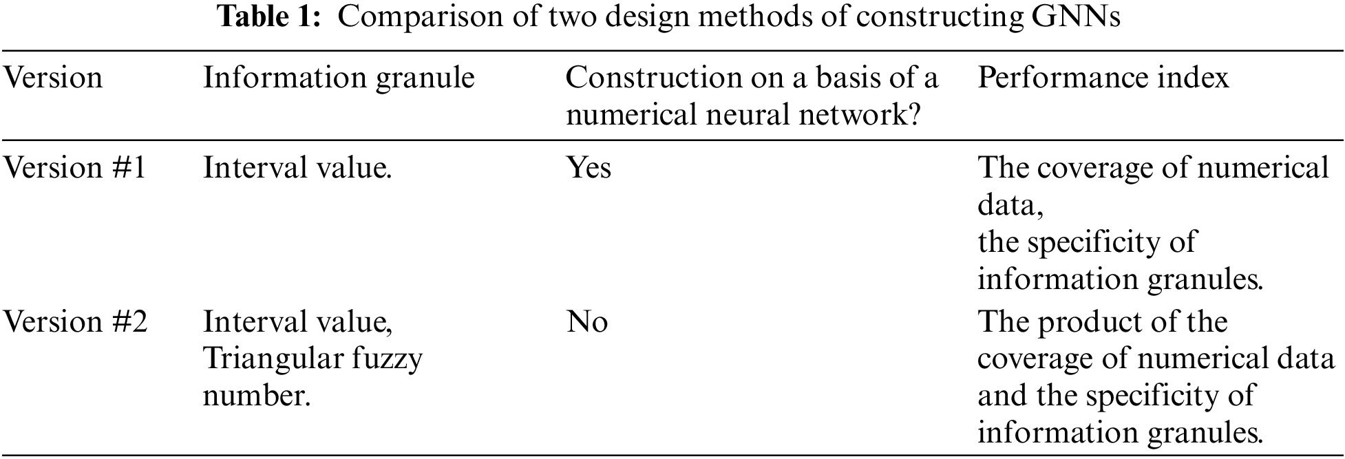
In this paper, the GNN based on an NNN is designated as Version #1, while the GNN independent of an NNN is termed Version #2. The distinctions between these two approaches are summarized in Table 1. This paper diverges from existing interval-valued neural networks (IVNNs) by developing a method not reliant on an NNN. It introduces triangular fuzzy numbers as network weights. The use of information granules is recognized as a valuable tool in network design, with their optimization contributing to improved network structures. The performance indicator discussed combines the coverage of numerical data and the specificity of information granules, enhancing network quality. The integration of coverage and specificity establishes a robust optimization framework for the network. Fundamentally, introducing this new network model expands the practices of the original networks, presenting theoretically and practically viable algorithms.

The structure of this paper is as follows: Section 2 offers a literature review. In Section 3, we initially outline the operational rules for interval and triangular fuzzy numbers. Subsequently, we describe the structure of a granular (interval-valued) neural network based on an NNN, along with two performance indicators for evaluating the output and optimal allocation of information granularity. Section 4 combines these two performance indicators into a singular metric. Here, we detail a novel method for developing a GNN, culminating in adopting triangular fuzzy numbers as the form of information granularity. Section 5 briefly introduces PSO, utilized in our experiments. Section 6 presents experimental studies. As previously mentioned, in this paper, an interval-valued (triangular fuzzy number) neural network represents a specific type of GNN. Therefore, when referring to a neural network as interval-valued (triangular fuzzy number), these two terms are used interchangeably.

2  Literature Review

ANNs [1–3] exhibit several limitations in information processing. Firstly, the complexity of ANNs increases rapidly with the growth in data dimensionality. Secondly, ANNs struggle to handle non-numeric data, such as qualitative descriptors like “higher,” “small,” or “around 35 degrees.” Thirdly, the “black box” nature of these networks hinders their interpretability. Granular computing, an approach that addresses complex information, involves dividing information into segments according to specific rules, thereby simplifying computations. These segments, known as information granules (e.g., groups, fuzzy numbers, intervals, and classes) [15], enable granular computing to handle non-numeric data. Original data are processed using numeric calculations, while granular data utilize granular computing mechanisms. This method allows for solving problems hierarchically [16–18]. Information granules can enhance the explainability of neural networks and address the challenges of ANNs. An ANN incorporating granular computing to improve existing models is termed a GNN. Examples include neural networks with granular structures and those capable of processing granular data without such structures [1,4].

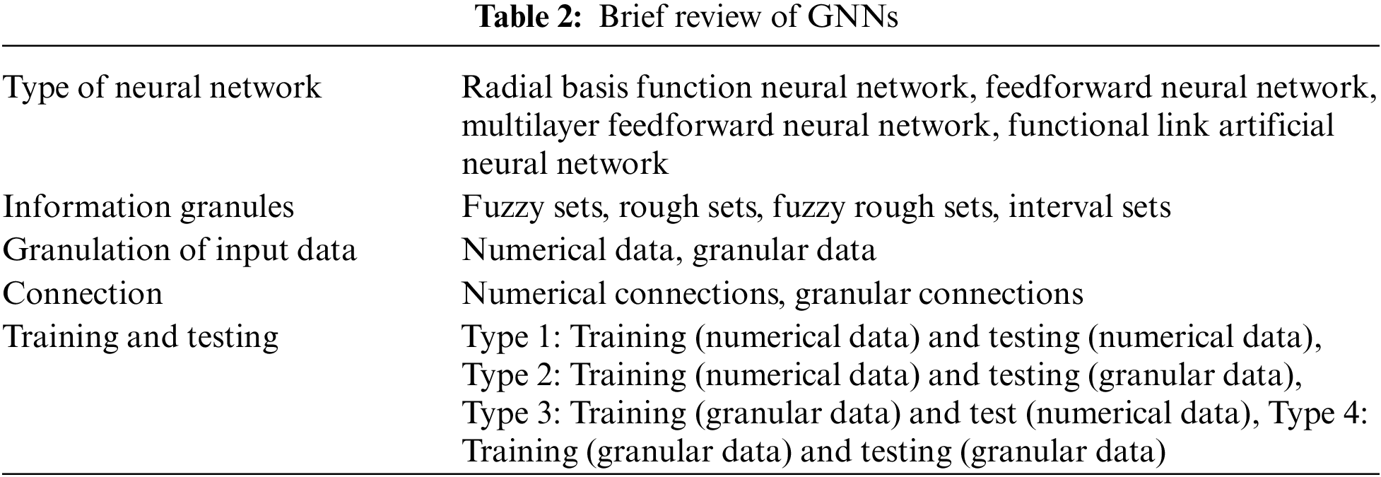
The initial concept of GNN, combining fuzzy sets with neural networks, emerged in the 1970s [19]. The term “granular neural network” was formally introduced in 2001 by Pedrycz et al. [4]. Since then, GNN research has garnered significant interest, as evidenced in Table 2. Studies on GNNs can be categorized into:

•   Type of neural network: Various neural network models, such as radial basis function neural networks [20,21], feedforward neural networks [7,22], multilayer feedforward neural networks [23,24], and functional link ANNs [25], are employed in GNN development.

•   Information granules: Granular computing, a paradigm of information processing [8,9], uses granules comprising elements with similar attributes. Various formal frameworks, including fuzzy sets [20,26,27], rough sets [22,28,29], fuzzy rough sets [30], and interval sets [7], can form these granules, leading to diverse GNN types like fuzzy neural networks, rough neural networks, and IVNNs.

•   Granulation of input data: Literature generally divides this aspect into two scenarios. In one, the input data are already at a granular level, requiring no further granulation. Conversely, numerical data are converted into forms like interval data or fuzzy numbers, sometimes employing clustering methods for division into several parts.

•   Connection: Traditional neural networks use numerical weights to represent their connections. In contrast, GNNs may employ nonnumerical weights, known as granular connections [5]. This distinction prompts researchers to explore modifications to traditional training methods, adapting them to GNNs’ unique structures. When GNNs receive numerical input data, they can produce nonnumerical outputs. Furthermore, GNNs can process nonnumerical input data in more complex scenarios. Some studies are investigating the use of primitive neural networks for processing nonnumerical data [31], maintaining the network’s original structure in such cases.

•   Training and testing. While traditional neural networks process numeric input during training and testing phases, GNNs with granular connections are trained on numerical data and tested on granular data. Additionally, the degree of data integration influences the granularity level; lower integration corresponds to finer granularity and higher integration results in coarser granularity. Notably, networks designed for low-granularity data may sometimes handle high-granularity data. This means the neural networks possess a low-granularity structure but can process high-granularity inputs during testing. A more frequent scenario involves inputting low-granularity data into a network designed for low-granularity processing.

Numerous GNN models have been developed to address specific challenges. For instance, in [32], researchers devised a nonlinear granularity mapping model with adaptive tuning factors to counteract unknown nonlinearity. In [33], a novel dynamic integration method was introduced to construct reliable prediction intervals for granular data streams, incorporating a new interval value learning algorithm applicable to fuzzy neural networks. In [34], a fuzzy-informed network was developed specifically for magnetic resonance imaging (MRI) image segmentation, utilizing fuzzy logic to encode input data. Additionally, a method using adaptive granular networks was designed for enhanced accuracy in sludge bulking detection [35]. This approach effectively creates an error compensation model. Furthermore, several GNNs incorporate local models, resulting in what are referred to as crisp neural networks [36,37]. These developments illustrate the versatility and adaptability of GNNs in various applications, ranging from image processing to environmental monitoring.

3  Two-Stage Design Process: Granularity Expansion of NNN

In this section, we initially present operations involving intervals and triangular fuzzy numbers. Subsequently, in Section 3.3, we delve into the existing IVNNs.

3.1 Interval Operations

We consider several interval-valued variables, such as A = [a1, a2] and B = [b1, b2], and outline their operations as follows [38]:

Addition:

A+B=[a1+b1,a2+b2](1)

Subtraction:

A−B=[a1−b2,a2−b1](2)

Multiplication:

A∗B=[min(a1b1,a1b2,a2b1,a2b2),max(a1b1,a1b2,a2b1,a2b2)](3)

when a1≥0,b1≥0,

A∗B=[a1b1,a2b2](4)

Division (except for cases where the divisor includes 0):

1A=[1a2,1a1](5)

BA=B∗1A=[b1,b2]∗[1a2,1a1](6)

In addition to interval operations, we also address the mapping (function) of intervals, particularly focusing on operations for nondecreasing mappings.

f(A)=f([a1,a2])=[f(a1),f(a2)](7)

For nonincreasing mapping, we obtain:

f(A)=f([a1,a2])=[f(a2),f(a1)](8)

3.2 Triangular Fuzzy Number

For the sake of space efficiency, we introduce only those parts [39] that are relevant to this paper.

Let A~ be a convex fuzzy set on the real number set R, if it has such a membership function:

μA~(x)={0x<ax−ab−aa<x<bx−cb−cb<x<c0x>c(9)

A~ is a triangular fuzzy number, where μA~(x):R→[0,1], a ≤ b ≤ c. If a=b=c, A~ is a real number.

Given triangular fuzzy numbers A~=(a,b,c) and B~=(d,e,f) their ∂−cut sets are expressed as A~={[(b−a)∂+a,(b−c)∂+c]}, B~={[(e−d)∂+d,(e−f)∂+f]}, which are intervals. Hence, they obey the operation rules applicable to interval operations, implying they can be manipulated like interval values.

3.3 Existing IVNNs

Initially, we construct NNNs in a supervised manner, utilizing a set of input-output pairs (xk, targetk), where k = 1, 2, …, N. These networks feature a classic MLP (multilayer perceptron) structure [40], representing a fundamental topology for feedforward neural networks. This paper employs the Levenberg-Marquardt BP (back propagation) learning method [41] as the learning mechanism. Through the learning process, a collection of weights is determined. Succinctly, the network is represented as (N(x; W)), with (W) denoting the network’s weights, where each weight is represented by (w_i). The subsequent phase involves the granulation of weights. Specifically, an interval is constructed around each (w_i), with the interval’s size (or length) determined by a parameter representing an information granularity level. Fig. 1 illustrates the structure of a GNN [7], evolved from a classic feedforward neural network. It consists of three layers: An input layer, where data features are inputted as a vector x = [x1,x2,…,xn]T; a hidden layer, containing n1 neurons; and an output layer with only one neuron. In an NNN, the weights connecting the input layer to the hidden layer are typically denoted by Wji, and those connecting the hidden layer to the output layer by Wj. Each connection includes a bias Bj. For the GNN, both the connection weights and biases are substituted with intervals Wji=[wji−,wji+], Wj=[wj−,wj+], and Bj=[bj−,bj+]. Consequently, when numeric data is inputted into this network, the output is an interval Y=[y−,y+].

Figure 1: Architecture of a GNN

After constructing the NNN, it is necessary to convert the network nodes into interval values. The procedures are detailed below. In the hidden layer of an NNN, the following is observed:

oj=f1(zj),zj=∑i=1nwji∗xi+bj,j=1,2,…,n1,i=1,2,…,nf1(zj)=11+e−zj(10)

For the output layer of the network, we obtain:

y=f2(z),z=∑j=1n1wj∗oj+b,f2(z)=z(11)

where wji denotes the weight from the input layer to the hidden layer, bj denotes the bias from the input layer to the hidden layer, b denotes the bias from the hidden layer to the output layer, wj denotes the weight from the hidden layer to the output layer, f1 and f2 represent the activation functions of the neuron from the input layer to the hidden layer and from the hidden layer to the output layer, respectively. oj denotes the output of a hidden layer, and y denotes the output of the network.

The subsequent section discusses the granulation of connections. The network is assigned an information granularity level ε, and connections are substituted with interval values. The weights wji,wj and biases bj are replaced by the interval generalizations:

w−=w−ε−|w|w+=w+ε+|w|bj−=bj−ε−|bj|bj+=bj+ε+|bj|(12)

Herein, we adopt a uniform allocation of information granularity to construct interval connections (granular connections) centered on the initial weights and biases. The intervals are symmetrically distributed around the original numeric value of each connection, implying that ε− = ε+ = ε/2. By substituting ε− = ε+ = ε/2 into the above equations, we obtain:

w−=w−ε−|w|=w−ε/2∗|w|=max(w(1−ε/2),w(1+ε/2))w+=w+ε+|w|=w+ε/2∗|w|=max(w(1−ε/2),w(1+ε/2))bj−=bj−ε−|bj|=bj−ε/2∗|bj|=min(bj(1−ε/2),bj(1+ε/2))bj+=bj+ε+|bj|=bj+ε/2∗|bj|=max(bj(1−ε/2),bj(1+ε/2))(13)

w−=min(w(1−ε/2),w(1+ε/2))w+=max(w(1−ε/2),w(1+ε/2))bj−=min(bj(1−ε/2),bj(1+ε/2))bj+=max(bj(1−ε/2),bj(1+ε/2))(14)

where ε is within the range of (0,1].

Substituting Eq. (14) into Eqs. (10) and (11) and replacing connections with interval values, we arrive at the following operations.

For the hidden layer:

oj=[oj−,oj+]=[f1(zj−),f1(zj+)]zj−=∑i=1n(min(wji−xi,wji+xi)+bj−)zj+=∑i=1n(max(wji−xi,wji+xi)+bj+),j=1,2,…,n1(15)

For the output layer:

Y=[y−,y+]=[f2(z−),f2(z+)]z−=∑i=1n(min(wj−oi−,wj+oi−,wj−oi+,wj+oi+)+bj−)z+=∑i=1n(max(wj−oi−,wj+oi−,wj−oi+,wj+oi+)+bj+),j=1,2,…,n1(16)

Since the network’s output is an interval, two performance indices are defined for evaluation purposes. The first is coverage, an index that indicates how many actual output intervals can ‘cover’ the expected output. The second is specificity, an index reflecting the average length of the output interval.

For any data (xk, targetk), where k = 1, 2, ⋯, n, in a dataset, when the network’s input is xk, the network produces an interval result Yk=[y k−,y k+]. The quality of the results is evaluated in terms of coverage and specificity. The measures are defined as follows:

Coverage: For any data (xk, targetk) and the output of the network Yk, if targetk ∈ Yk, then Yk ‘covers’ targetk. Coverage quantifies the ratio of the number of data points covered to the total data amount.

Q1(ε)=1N∑k=1Nincl(targetk,Yk)(17)

where

incl(targetk,Yk)={1 if targetk∈[yk−,yk+]0,otherwise(18)

Specificity: It quantifies the average length of output intervals:

where the range = |targetmax-targetmin|.

To summarize the discussion, the process can be delineated as follows:

Phase 1: Utilize the provided data to derive a new neural network employing numeric data and the backpropagation method.

Phase 2: Assign an information granularity level ε to the NNN constructed in the first phase, converting the numerical connection into an information granularity connection (interval value).

Phase 3: Optimize the objective function to identify the best parameters using PSO.

Phase 4: Construct the IVNN using the weights from the original NNN and the optimized information granularity level ε.

4  Single-Phase Design of GNN

Specificity (Q2) calculates the average length of output intervals, and coverage (Q1) assesses how many actual output intervals can ‘cover’ the expected output. These performance indices articulate and quantify information granularity in distinct manners. Based on the definitions of these performance indices, superior values indicate enhanced network performance. To thoroughly compare two methodologies for constructing a GNN, the product of the two performance indices of coverage and specificity is considered the objective function for the network. This novel performance index aptly balances the two indices. Consequently, the optimal values for the network parameters are determined by maximizing this new objective function, enhancing the network’s adaptability.

V(ε)=Q1(ε)∗Q2(ε)(20)

where ε is a non-negative value, with εmax denoting the maximum allowable value of ε.

Considering the range of values of ε, a global performance index is formulated as:

S(W)=∫01V(ε)dε(21)

For ε within the range of (0,1], where the level of information granules is within the unit interval, W represents the weights and biases of the network. In practical applications, integration is substituted with summation.

Given the nature of the performance index, it is clear that optimization cannot be limited to gradient-based methods. Therefore, PSO is considered for the optimization challenges presented [9,10].

As previously mentioned, the weights derived from the numeric neural network in phase 1, along with the ε that provides the best coverage and specificity for these weights, are not necessarily the optimal parameters for achieving high coverage and specificity. Consequently, a different strategy is adopted to develop a GNN. This approach involves combining the first and second phases of the earlier algorithm. In essence, instead of calculating the weights beforehand, the objective function V is optimized directly to simultaneously determine all parameters.

With this approach, the construction of the connections is also modified:

w−=min(w11+ε,w(1+ε))w+=max(w11+ε,w(1+ε))bj−=min(bj11+ε,bj(1+ε))bj+=max(bj11+ε,bj(1+ε))(22)

Triangular fuzzy numbers, which express uncertainty effectively, are frequently utilized as information granules in granular computing. Their cut sets can be converted into a series of intervals, allowing the use of interval values in the construction and performance evaluation of a GNN.

Regardless of the type of information granule—whether interval values or triangular fuzzy numbers—the steps for constructing these two variations of GNNs remain consistent. The GNN derived from an NNN is designated as Version #1, whereas the GNN developed independently of an NNN is referred to as Version #2. The methods for constructing a GNN are concisely outlined. Figs. 2 and 3 illustrate the algorithmic flow of each version.

Figure 2: Flow of the construction of Version #1

Figure 3: Flow of the construction of Version #2

Procedure for the construction of Version #1.

Procedure for the construction of Version #2.

Phase 1: For a neural network with undetermined parameters, establish an information granularity level ε, converting the network’s connections into information granularity connections (interval values or triangular fuzzy numbers).

Phase 2: Input the provided data into the network and derive the objective function V, which depends on the network parameters. Optimize this objective function to identify the optimal network parameters.

Phase 3: Utilize the optimized parameters to establish the information granular connections of the network (using interval values or triangular fuzzy numbers), thereby constructing the GNN. Consequently, a granular network is developed.

5  PSO

In the optimization of neural networks, PSO was employed as an optimizer. A concise summary of its algorithm flow is provided below. Recognizing the distinct advantages inherent in various algorithms, integrating these methodologies has emerged as a significant focus of research aimed at overcoming the limitations of individual approaches. Prominent algorithms for hybrid computation have included the ant colony algorithm, genetic algorithm, and simulated annealing, among others. PSO emerged as a robust optimization algorithm capable of working with nonconvex models, logical models, complex simulation models, black box models, and even real experiments for optimization calculations. In PSO, each particle represented a potential solution consisting of a vector of optimized levels of information granularity, weights, and biases. The problem-solving intelligence was realized through simple behaviors and information exchanges among particles and particle swarms. The procedure was as follows:

Phase 1: Initialization involved setting the maximum number of iterations, the number of independent variables in the objective function, the maximum velocity of particles, and their location information across the entire search space. The speed and location were randomly initialized within the speed interval and search space, respectively. The population size of the particle swarm was also established.

Phase 2: Individual extremum and global optimum. A fitness function was defined. The individual extremum referred to the optimal solution found by each particle, while the global optimum was determined from the best solutions identified by all particles. This global optimum was then compared with historical optima, and the best was selected as the current historical optimal solution.

Phase 3: The velocity and position were updated according to:

vid=w∗vid+c1∗r1(pbestid−xid)+c2∗r2(gbestid−xid)xid=xid+vid(23)

where w denotes the inertia factor influencing the convergence of the swarm, c1 and c2 are the learning factors for adjusting the maximum learning phase size, i denotes the first particle, and d denotes the dimensionality of the particle. r1 and r2 are two random numbers in the range [0,1] (for different particle sizes, the values of r1and r2vary), pbestid denotes the position where the particle achieves its highest (lowest) fitness, and gbestid denotes the position where the entire system achieves its highest (lowest) fitness.

6  Experimental Studies

Multiple datasets were utilized, and a series of experiments were conducted to compare the performance of the newly proposed GNN in this study with existing GNNs. All datasets, including synthetic and benchmark datasets, were sourced from the UCI Machine Learning Repository (http://archive.ics.uci.edu/datasets). To evaluate the performance of numeric neural networks, the root mean squared error (RMSE) was employed as the indicator. A 10-fold cross-validation was introduced to generate the training and testing datasets.

In this study, both IVNNs and triangular fuzzy number neural networks shared the same network structure; the only difference lay in the information granules of the network nodes. These neural networks had only one hidden layer and a single output node. A series of experiments were also conducted to examine the relationship between network performance and the number of nodes in the hidden layer. The NNN was trained using the standard Levenberg-Marquardt minimization method, with the number of generations set to 1000. Before initiating the network, data preprocessing was performed to ensure that different dimensions of multidimensional data played the same role. The initial weights for all networks were set between [−1, 1]. The activation function for the input layer was sigmoid, while that for the hidden layer was linear.

A method described in previous sections was employed to construct a new network to test its performance, utilizing 10-fold cross-validation for data processing. Following the methodology in [42], the parameters of PSO were initialized with the number of generations set to 100, w to 0.7, c1 to 2, and c2 to 2. Adjusting different initial parameters did not yield any significant change in network performance, leading to the adoption of these parameters for all networks. The training time was also documented due to significant differences in training costs when using different information granules to construct the network.

Table 3 presents the datasets used in this study, all of which are regression.

6.1 Synthetic Data

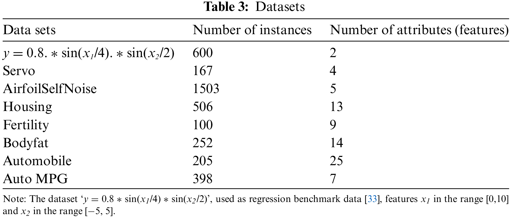
These two-dimensional synthetic data, derived from the regression benchmark dataset [43], are modeled by the following nonlinear function f (x1, x2):

f(x1,x2)=0.8∗sin⁡(x1/4).∗sin⁡(x2/2)+z(24)

where z is obtained from the Gaussian normal distribution N (0, 0.2). A total of 600 sets of random data, adhering to a uniform distribution, were generated. The visualization of these 600 datasets is depicted in Fig. 4.

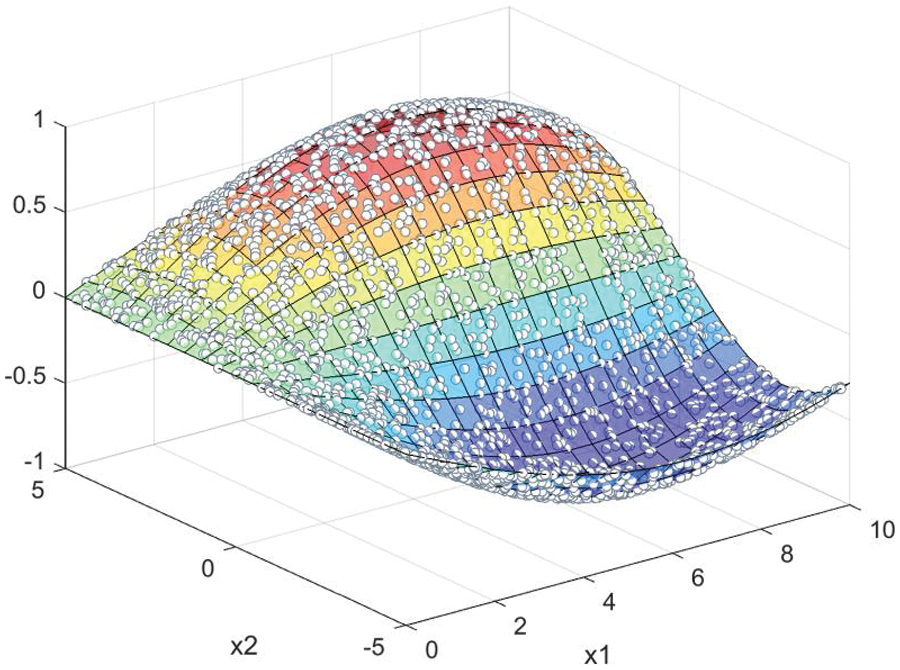
Figure 4: Two dimensional nonlinear function ‘y = 0.8 * sin(x1/4) * sin(x2/2)’ used in the experiment

We consider an MLP with only one hidden layer of size h. Training is conducted using a standard BP algorithm. The performance of the NNN, as a function of h, is illustrated in Fig. 5; the size of h varies from 2 to 10. An optimal value of h is determined when the performance index reaches its minimum value. According to Fig. 5, the optimal h is 8. Subsequently, a new network featuring granular connections is constructed by selecting its ε value within the range (0, 1] for Version #1 and in the range (0, 10] for Version #2.

Figure 5: RMSE vs. h (number of neurons in hidden layer): Training data (red line) and testing data (black line)

Fig. 6 illustrates the variations in the objective functions V, Q1, and Q2 when ε is within the range (0,1]. Notably, irrespective of whether the information granule is an interval value or a triangular fuzzy number, the change tendency of these objective functions remains the same when the construction approach (Version #1 or Version #2) of the network is consistent.

Figure 6: Q1, Q2, and V vs. ε (ε is in (0, 1]); solid line—training data; dotted line—testing data

For a GNN of Version #1, the optimal number of neurons in the hidden layer is determined to be 8. However, as shown in Table 4, for the same dataset in the Version #2 neural network, whether interval or triangular fuzzy number-valued, h is found to be 4. According to Table 5, the performance indices V and S for Version #2, both for interval-valued and triangular fuzzy number-valued neural networks, are significantly better than those for the IVNN of Version #1. This aligns with prior analyses. Additionally, the IVNN of Version #2 demonstrates superior performance across all indices.

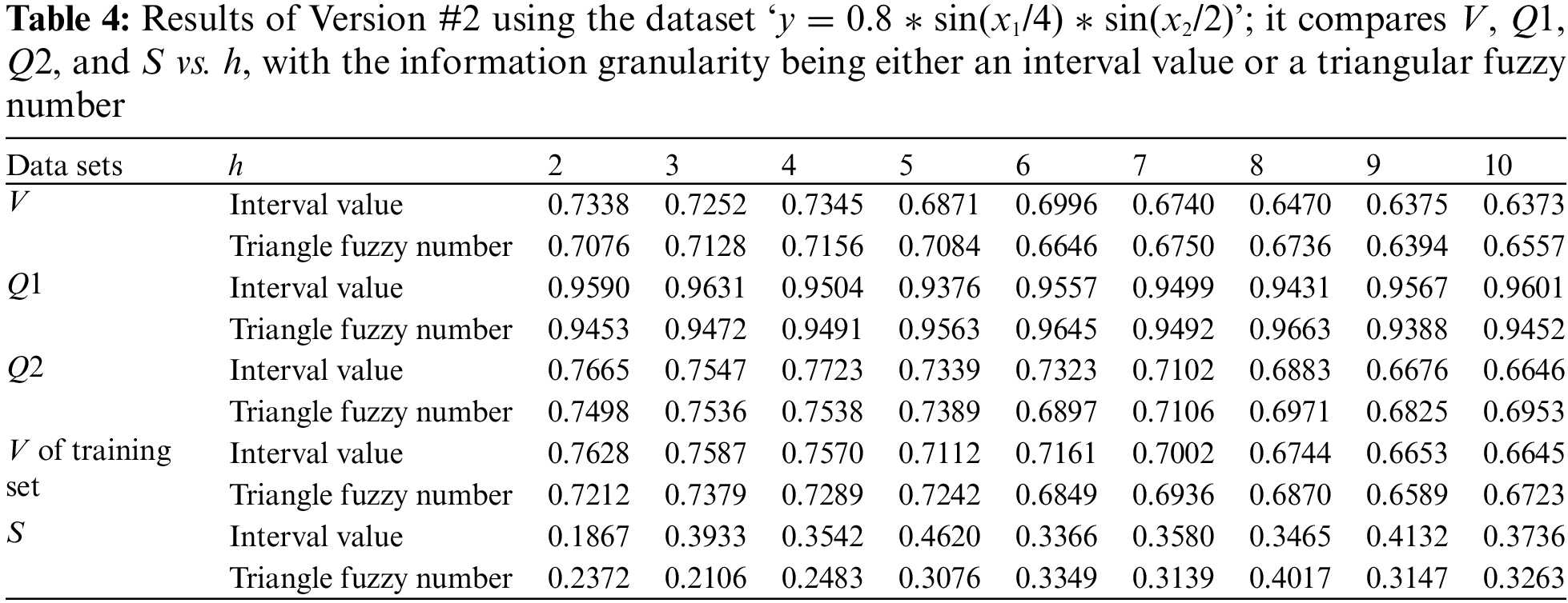
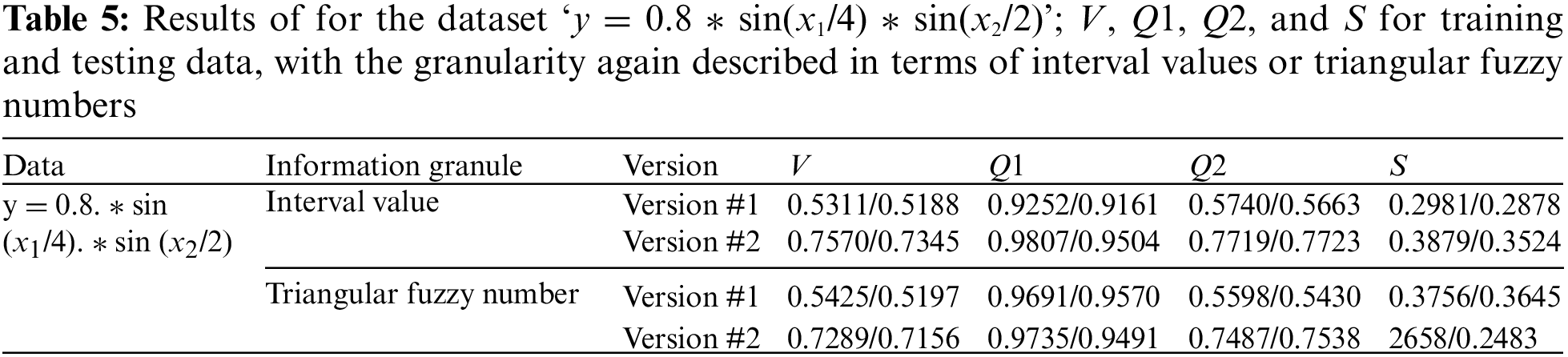
For Version #1, the V (for both training and testing sets) and S indices obtained by the triangular fuzzy number-valued network are slightly better than those from the interval-valued network. Conversely, for Version #2, the IVNNs outperform the triangular fuzzy number-valued networks in terms of V and S. The experimental results from this dataset do not conclusively determine whether the performance of IVNNs surpasses that of triangular fuzzy number neural networks with identical network structures, whether Version #1 or Version #2, or the reverse.

Furthermore, no regular pattern was observed in how the performance indices V and S change with variations in the number of nodes in the hidden layer. This suggests that the new GNNs proposed in this paper are feasible and perform better. To further validate these findings, experiments will be conducted on the seven datasets listed on the left side of Table 3 in the following section.

Fig. 7 provides an intuitive comparison of the performance of the four GNNs. The vertical lines in the figures indicate the network outputs (intervals, triangular fuzzy numbers), with a shorter average length correlating with a better Specificity index. Outputs that cover the theoretical outputs are marked with a slash across the vertical lines, indicating that more lines crossed by a slash signify a better Coverage index.

Figure 7: Dataset ‘y = 0.8 * sin(x1/4) * sin(x2/2)’; x-axis—target output; y-axis—actual output (interval value/triangular fuzzy number value)

Fig. 8 presents the evolution of the fitness functions across 100 generations. Notably, the triangular fuzzy number-valued neural network for Version #2 exhibits the quickest convergence, achieving this within the initial twenty generations.

Figure 8: Fitness function of PSO in 100 generations

6.2 Publicly Available Data from the Machine Learning Repository

The performances of the constructed networks, functioning as variables of h, are illustrated in Fig. 9, where the size of h varies from 2 to 10. In version #1, irrespective of the GNN’s utilization of interval values or triangular fuzzy numbers, h is assigned values of 2, 10, 10, 10, 2, 2, and 3 for the datasets Servo, Airfoil Self Noise, Housing, Fertility, Bodyfat, Automobile, and Auto MPG, respectively.

Figure 9: RMSE vs. h (number of neurons in hidden layer): Interval-valued/triangular fuzzy number-valued neural network (Version #1); training data (red line) and testing data (black line)

The index V, obtained by the constructed neural networks for Version #2 and quantified with respect to the number of neurons in the hidden layer, is displayed in Figs. 10 and 11. For the datasets Servo, Airfoil Self Noise, Housing, Fertility, Bodyfat, Automobile, and Auto MPG, the optimal h values for the interval-valued network are 3, 5, 8, 2, 5, 3, and 2, respectively, and for the triangular fuzzy number network, they are 3, 6, 2, 2, 10, 2, and 3, respectively. Consistent with the preceding section, there is no evidence to suggest that the performance index systematically varies as the number of neurons in the hidden layer changes.

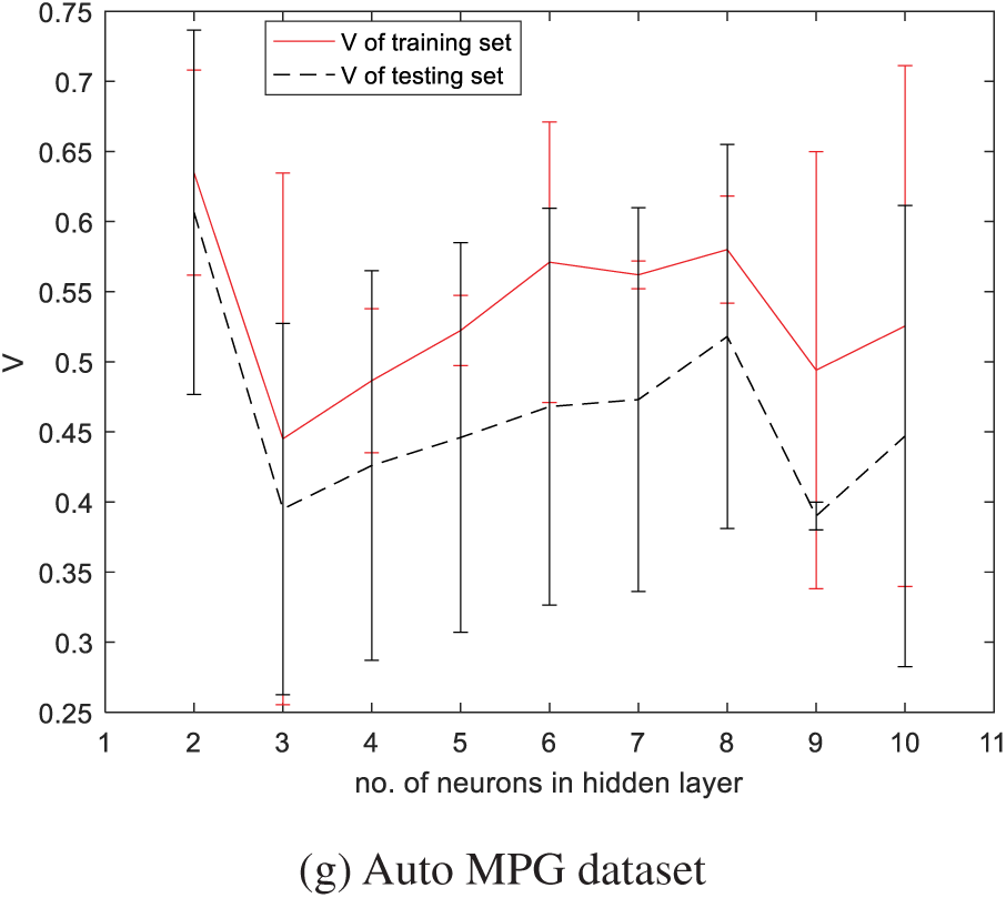
Figure 10: V vs. h (number of neurons in hidden layer): IVNN (Version #2)

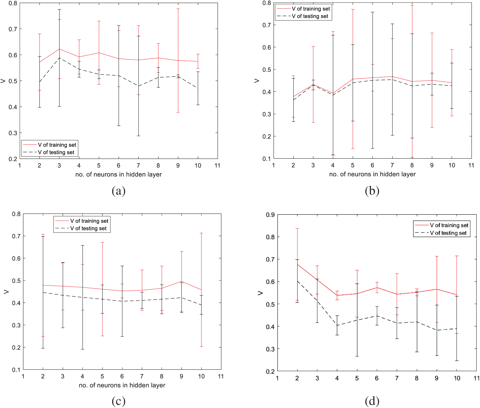
Figure 11: V vs. h (number of neurons in hidden layer): Triangular fuzzy number-valued neural network (Version #2)

The determination of the value of h is achieved by minimizing the performance index. Subsequently, with the determined value of h, a network is constructed by selecting the value of ε within the range (0,1] for Version #1 and (0,10] for Version #2.

The dataset ‘y = 0.8 * sin(x1/4) * sin(x2/2)’ has its experimental results previously discussed and visually represented in Fig. 12. The results of other data sets are all in Tables 6–12. Like earlier experiments, it can be concluded that for both training and testing sets, the indices V and S achieved by both interval-valued and triangular fuzzy number-valued neural networks for Version #2 surpass those obtained by the IVNN for Version #1. There is, however, no clear evidence to suggest a consistent superiority in performance between the interval-valued and triangular fuzzy number-valued neural networks when the network structure remains unchanged (whether for Version #1 or Version #2).

Figure 12: Plot of coverage, specificity, V, and S; solid line indicates training data; dotted line indicates testing data. Method 1 employs an IVNN for Version #1, Method 2 utilizes an IVNN for Version #2, Method 3 uses a triangular fuzzy number-valued neural network for Version #1, and Method 4 applies a triangular fuzzy number-valued neural network for Version #2

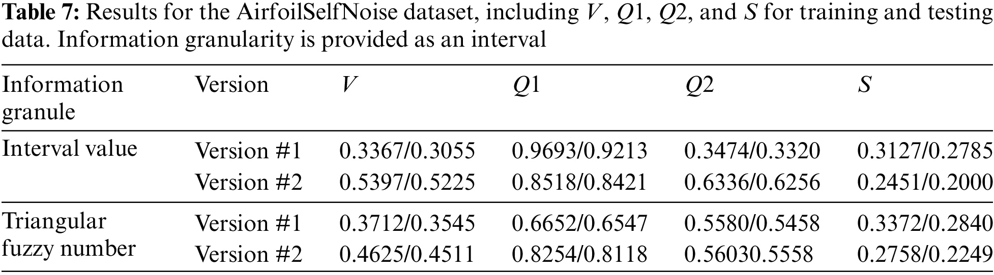
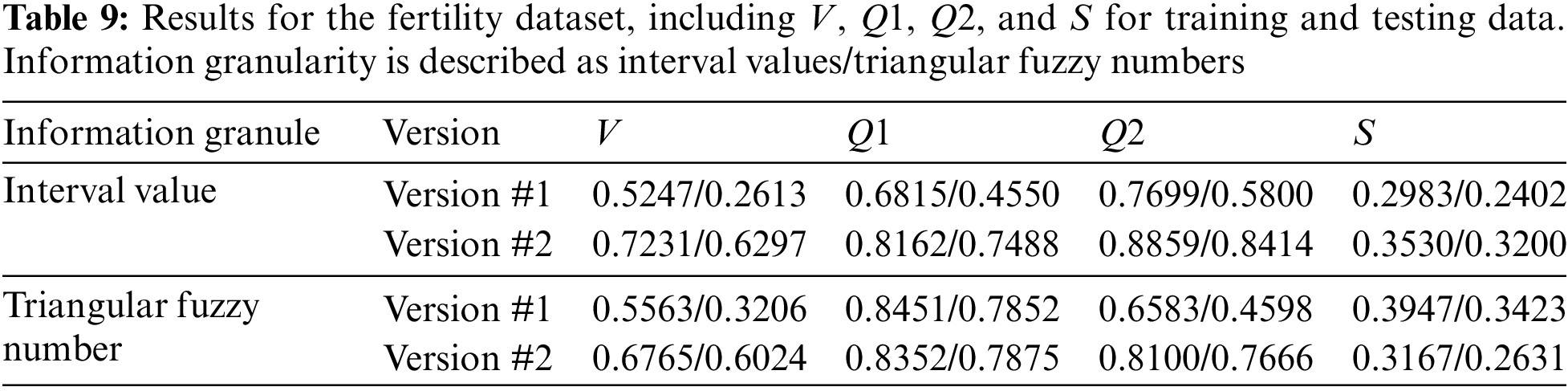
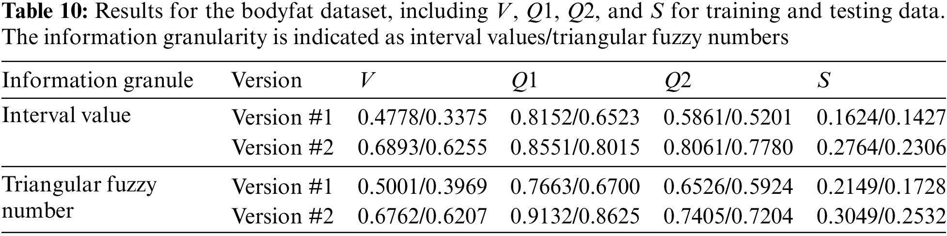
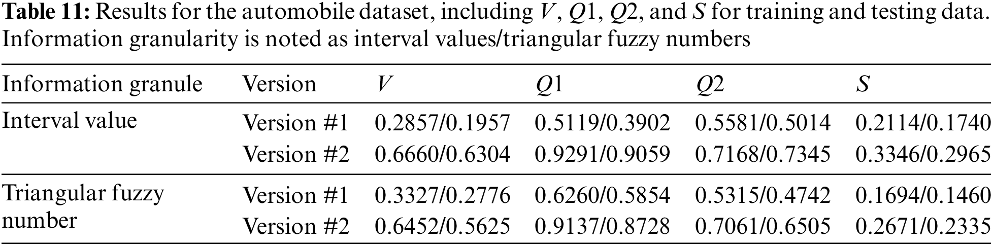
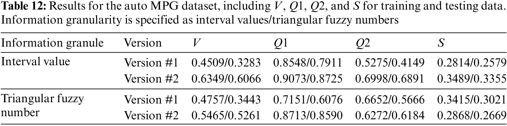
Nevertheless, other results indicate variable performances for indexes S and V. The IVNN for Version #2 shows the best performance for index V, while the triangular fuzzy number-valued neural network for Version #2 presents the second-best outcomes, except for the dataset ‘Servo’. Notably, the best values of S are predominantly achieved by the IVNNs for Version #2 and the triangular fuzzy number-valued neural networks for Version #1. For all datasets, the IVNNs for Version #1 did not attain the optimal S values.

7  Conclusions and Further Work

The broad application of deep learning technology has sparked significant interest in the structural design of neural networks. GNNs offer a novel perspective for network structure design and can handle various data types. These networks, characterized by their granular connections, output granular data, thus providing a novel method for achieving higher-level abstract results. The role of information granularity is crucial in the design process of neural networks.

This paper introduces several new granular networks, building upon an established GNN. The work is summarized as follows: Firstly, it integrates two performance indices into a new one to serve as the network’s performance index. Secondly, it optimizes the network directly to construct GNNs, moving away from NNNs. Thirdly, it explores the construction of connections using triangular fuzzy numbers. A series of experiments with synthetic and real data demonstrate that the new design scheme is viable and attains favorable performance indices.

Due to their simplicity, interval values and triangular fuzzy numbers are employed as the information granularity for granular connections. Exploring other forms of information granularity could offer alternatives for the network’s granularity structure. Moreover, GNNs are not restricted to a single network architecture; multilayer perceptrons could also be considered. However, substituting numerical connections in the original neural network with granular connections increases the number of network parameters, complicating network optimization. Gradient-based methods may offer a promising solution.

Acknowledgement: The authors would like to express their gratitude for the valuable feedback and suggestions provided by all the anonymous reviewers and the editorial team.

Funding Statement: This work is partially supported by the National Key R&D Program of China under Grant 2018YFB1700104.

Author Contributions: Conceptualization, Witold Pedrycz, Yushan Yin and Zhiwu Li; Data curation, Yushan Yin; Formal analysis, Yushan Yin and Witold Pedrycz; Investigation, Yushan Yin; Methodology, Yushan Yin, Witold Pedrycz and Zhiwu Li; Software, Yushan Yin; Validation, Witold Pedrycz and Yushan Yin; Visualization, Yushan Yin; Writing–original draft, Yushan Yin and Witold Pedrycz. All authors reviewed the results and approved the final version of the manuscript.

Availability of Data and Materials: All the data sets (synthetic data sets and benchmark data sets) are from the UCI Machine Learning Repository (http://archive.ics.uci.edu/datasets).

Conflicts of Interest: The authors declare that they have no known competing financial interests or personal relationships that could have appeared to influence the work reported in this paper.

References

1. M. Song and Y. Wang, “A study of granular computing in the agenda of growth of artificial neural networks,” Granul. Comput., vol. 1, no. 4, pp. 1–11, 2016. doi: 10.1007/s41066-016-0020-7. [Google Scholar] [CrossRef]

2. K. Liu, L. Chen, J. Huang, S. Liu, and J. Yu, “Revisiting RFID missing tag identification,” in IEEE Conf. Comput. Commun., London, UK, 2022, pp. 710–719. doi: 10.1109/INFOCOM48880.2022.9796971. [Google Scholar] [CrossRef]

3. E. Olmez, E. Eriolu, and E. Ba, “Bootstrapped dendritic neuron model artificial neural network for forecasting,” Granul. Comput., vol. 8, no. 6, pp. 1689–1699, 2023. doi: 10.1007/s41066-023-00390-1. [Google Scholar] [CrossRef]

4. W. Pedrycz and G. Vukovich, “Granular neural networks,” Neurocomput., vol. 36, no. 1–4, pp. 205–224, 2001. doi: 10.1016/S0925-2312(00)00342-8. [Google Scholar] [CrossRef]

5. M. Beheshti, A. Berrached, A. de Korvin, C. Hu, and O. Sirisaengtaksin, “On interval weighted three-layer neural networks,” in Proc. 31st Ann. Simul. Symp., Boston, MA, USA, 1998, pp. 188–194. doi: 10.1109/SIMSYM.1998.668487. [Google Scholar] [CrossRef]

6. H. Ishibuchi, H. Tanaka, and H. Okada, “An architecture of neural networks with interval weights and its application to fuzzy regression analysis,” Fuzzy Sets Syst., vol. 57, no. 1, pp. 27–39, 1993. doi: 10.1016/0165-0114(93)90118-2. [Google Scholar] [CrossRef]

7. S. Ridella, S. Rovetta, and R. Zunino, “IAVQ-interval-arithmetic vector quantization for image compression,” IEEE Trans. Circ. Syst. II: Analog Digit. Signal Process., vol. 47, no. 12, pp. 1378–1390, 2000. doi: 10.1109/82.899630. [Google Scholar] [CrossRef]

8. M. Song and W. Pedrycz, “Granular neural networks: Concepts and development schemes,” IEEE Trans. Neural Netw. Learn. Syst., vol. 24, no. 4, pp. 542–553, 2013. doi: 10.1109/TNNLS.2013.2237787. [Google Scholar] [PubMed] [CrossRef]

9. S. Nabavi-Kerizi, M. Abadi, and E. Kabir, “A PSO-based weighting method for linear combination of neural networks,” Comput. Electric. Eng., vol. 36, no. 5, pp. 886–894, 2012. doi: 10.1016/j.compeleceng.2008.04.006. [Google Scholar] [CrossRef]

10. T. M. Shami, A. A. El-Saleh, M. Alswaitti, Q. Al-Tashi, M. A. Summakieh and S. Mirjalili, “Particle swarm optimization: A comprehensive survey,” IEEE Access, vol. 10, pp. 10031–10061, 2022. doi: 10.1109/ACCESS.2022.3142859. [Google Scholar] [CrossRef]

11. Z. Anari, A. Hatamlou, and B. Anari, “Automatic finding trapezoidal membership functions in mining fuzzy association rules based on learning automata,” Int. J. Interact. Multimed. Artif. Intell., vol. 7, no. 4, pp. 27–43, 2022. doi: 10.9781/ijimai.2022.01.001. [Google Scholar] [PubMed] [CrossRef]

12. Y. N. Pawan, K. B. Prakash, S. Chowdhury, and Y. Hu, “Particle swarm optimization performance improvement using deep learning techniques,” Multimed. Tool Appl., vol. 81, no. 19, pp. 27949–27968, 2022. doi: 10.1007/s11042-022-12966-1. [Google Scholar] [CrossRef]

13. C. Fonseca and P. Fleming, “Multiobjective optimization and multiple constraint handling with evolutionary algorithms. I. A unified formulation,” IEEE Trans. Syst., Man, Cybernet.—Part A: Syst. Human., vol. 28, no. 1, pp. 26–37, 1998. doi: 10.1109/3468.650319. [Google Scholar] [CrossRef]

14. H. Rezk, J. Arfaoui, and M. R. Gomaa, “Optimal parameter estimation of solar PV panel based on hybrid particle swarm and grey wolf optimization algorithms,” Int. J. Interact. Multimed. Artif. Intell., vol. 6, no. 6, pp. 145–155, 2021. doi: 10.9781/ijimai.2020.12.001. [Google Scholar] [PubMed] [CrossRef]

15. L. A. Zadeh and J. Kacprzyk, “Words about uncertainty: Analogies and contexts,” in Computing with Words in Information Intelligent Systems, Heidelberg, Germany: Physica-Verlag, 1999, pp. 119–135. [Google Scholar]

16. W. Pedrycz and M. Song, “Analytic hierarchy process (AHP) in group decision making and its optimization with an allocation of information granularity,” IEEE Trans. Fuzzy Syst., vol. 19, no. 3, pp. 527–539, 2011. doi: 10.1109/TFUZZ.2011.2116029. [Google Scholar] [CrossRef]

17. Z. Kuang, X. Zhang, J. Yu, Z. Li, and J. Fan, “Deep embedding of concept ontology for hierarchical fashion recognition,” Neurocomput., vol. 425, no. 4, pp. 191–206, 2020. doi: 10.1016/j.neucom.2020.04.085. [Google Scholar] [CrossRef]

18. Y. Wan, G. Zou, C. Yan, and B. Zhang, “Dual attention composition network for fashion image retrieval with attribute manipulation,” Neural Comput. Appl., vol. 35, no. 8, pp. 5889–5902, 2023. doi: 10.1007/s00521-022-07994-9. [Google Scholar] [CrossRef]

19. S. Lee and E. Lee, “Fuzzy sets and neural networks,” J. Cybernet., vol. 4, no. 2, pp. 83–103, 1974. doi: 10.1080/01969727408546068. [Google Scholar] [CrossRef]

20. A. M. Abadi, D. U. Wutsqa, and N. Ningsih, “Construction of fuzzy radial basis function neural network model for diagnosing prostate cancer,” Telkomnika (Telecommun. Comput. Electron. Control), vol. 19, no. 4, pp. 1273, 2021. doi: 10.12928/telkomnika.v19i4.20398. [Google Scholar] [CrossRef]

21. S. A. Shanthi and G. Sathiyapriya, “Universal approximation theorem for a radial basis function fuzzy neural network,” Mater. Today: Proc., vol. 51, no. 4, pp. 2355–2358, 2022. doi: 10.1016/j.matpr.2021.11.576. [Google Scholar] [CrossRef]

22. K. H. Chen, L. Yang, J. P. Wang, S. I. Lin, and C. L. Chen, “Automatic manpower allocation for public construction projects using a rough set enhanced neural network,” Canadian J. Civil Eng., vol. 1, no. 8, pp. 1020–1025, 2020. doi: 10.1139/cjce-2019-0561. [Google Scholar] [CrossRef]

23. M. Song, L. Hu, S. Feng, and Y. Wang, “Feature ranking based on an improved granular neural network,” Gran. Comput., vol. 8, no. 1, pp. 209–222, 2023. doi: 10.1007/s41066-022-00324-3. [Google Scholar] [CrossRef]

24. M. Wang et al., “Data-driven strain-stress modelling of granular materials via temporal convolution neural network,” Comput. Geotechn., vol. 152, no. 5, pp. 105049, 2022. doi: 10.1016/j.compgeo.2022.105049. [Google Scholar] [CrossRef]

25. N. M. Lanbaran and E. Elik, “Prediction of breast cancer through tolerance-based intuitionistic fuzzy-rough set feature selection and artificial neural network,” Gazi Univ. J. Sci., 2021. doi: 10.35378/GUJS.857099. [Google Scholar] [CrossRef]

26. A. Hakan, C. Resul, T. Erkan, D. Besir, and K. Korhan, “Advanced control of three-phase PWM rectifier using interval type-2 fuzzy neural network optimized by modified golden sine algorithm,” IEEE Trans. Cybernet., vol. 52, no. 5, pp. 2994–3005, 2023. doi: 10.1109/TCYB.2020.3022527. [Google Scholar] [CrossRef]

27. H. J. He, X. Meng, J. Tang, and J. F. Qiao, “Event-triggered-based self-organizing fuzzy neural network control for the municipal solid waste incineration process,” Sci. China Technol. Sc., vol. 66, pp. 1096–1109, 2023. [Google Scholar]

28. J. Cao, X. Xia, L. Wang, and Z. Zhang, “A novel back propagation neural network optimized by rough set and particle swarm algorithm for remanufacturing service provider classification and selection,” J. Phys.: Conf. Series, vol. 2083, no. 4, pp. 042058, 2021. doi: 10.1088/1742-6596/2083/4/042058. [Google Scholar] [CrossRef]

29. A. Sheikhoushaghi, N. Y. Gharaei, and A. Nikoofard, “Application of rough neural network to forecast oil production rate of an oil field in a comparative study,” J. Pet. Sci. Eng., vol. 209, no. 1, pp. 109935, 2022. doi: 10.1016/j.petrol.2021.109935. [Google Scholar] [CrossRef]

30. A. Kumar and P. S. V. S. S. Prasad, “Incremental fuzzy rough sets based feature subset selection using fuzzy min-max neural network preprocessing,” Int. J. Approx. Reason., vol. 139, no. 3, pp. 69–87, 2021. doi: 10.1016/j.ijar.2021.09.006. [Google Scholar] [CrossRef]

31. A. Vasilakos and D. Stathakis, “Granular neural networks for land use classification,” Soft Comput., vol. 9, no. 5, pp. 332–340, 2005. doi: 10.1007/s00500-004-0412-5. [Google Scholar] [CrossRef]

32. Z. Yu et al., “Refined fault tolerant tracking control of fixed-wing UAVs via fractional calculus and interval type-2 fuzzy neural network under event-triggered communication,” Inf. Sci., vol. 644, no. 5, pp. 119276, 2023. doi: 10.1016/j.ins.2023.119276. [Google Scholar] [CrossRef]

33. Y. Liu, J. Zhao, W. Wang, and W. Pedrycz, “Prediction intervals for granular data streams based on evolving type-2 fuzzy granular neural network dynamic ensemble,” IEEE Trans. Fuzzy Syst., vol. 29, no. 4, pp. 874–888, 2021. doi: 10.1109/TFUZZ.2020.2966172. [Google Scholar] [CrossRef]

34. W. Ding, M. Abdel-Basset, H. Hawash, and W. Pedrycz, “Multimodal infant brain segmentation by fuzzy-informed deep learning,” IEEE Trans. Fuzzy Syst., vol. 30, no. 4, pp. 1088–1101, 2022. doi: 10.1109/TFUZZ.2021.3052461. [Google Scholar] [CrossRef]

35. L. Zhang, M. Zhong, and H. Han, “Detection of sludge bulking using adaptive fuzzy neural network and mechanism model,” Neurocomputing, vol. 481, pp. 193–201, 2022. doi: 10.3389/978-2-88974-540-1. [Google Scholar] [CrossRef]

36. D. Sánchez, P. Melin, and O. Castillo, “Optimization of modular granular neural networks using a hierarchical genetic algorithm based on the database complexity applied to human recognition,” Inf. Sci., vol. 309, no. 2, pp. 73–101, 2015. doi: 10.1016/j.ins.2015.02.020. [Google Scholar] [CrossRef]

37. D. Sánchez and P. Melin, “Optimization of modular granular neural networks using hierarchical genetic algorithms for human recognition using the ear biometric measure,” Eng. Appl. Artif. Intell., vol. 27, no. 11, pp. 41–56, 2014. doi: 10.1016/j.engappai.2013.09.014. [Google Scholar] [CrossRef]

38. E. Weerdt, Q. Chu, and J. Mulder, “Neural network output optimization using interval analysis,” IEEE Trans. Neural Netw., vol. 20, no. 4, pp. 638–653, 2009. doi: 10.1109/TNN.2008.2011267. [Google Scholar] [PubMed] [CrossRef]

39. M. Mizumoto and K. Tanaka, “The four operations of arithmetic on fuzzy numbers, systems computing,” Controls, vol. 7, no. 5, pp. 73–81, 1976. [Google Scholar]

40. M. Rocha, P. Cortez, and J. Neves, “Evolutionary design of neural networks for classification and regression,” in Adaptive Natural Computing Algorithms, Coimbra, Portugal, 2005, pp. 304–307. doi: 10.1007/3-211-27389-1_73. [Google Scholar] [CrossRef]

41. M. T. Hagan and M. B. Menhaj, “Training feedforward networks with the Marquardt algorithm,” IEEE Trans. Neural Netw., vol. 5, no. 6, pp. 989–993, 1994. doi: 10.1109/72.329697. [Google Scholar] [PubMed] [CrossRef]

42. E. Zitzler, K. Deb, and L. Thiele, “Comparison of multiobjective evolutionary algorithms: Empirical results,” Evol. Comput., vol. 8, no. 2, pp. 173–195, 2000. doi: 10.1162/106365600568202. [Google Scholar] [PubMed] [CrossRef]

43. D. Wedge, D. Ingram, D. McLean, C. Mingham, and Z. Bandar, “On global-local artificial neural networks for function approximation,” IEEE Trans. Neural Netw., vol. 17, no. 4, pp. 942–952, 2006. doi: 10.1109/TNN.2006.875972. [Google Scholar] [PubMed] [CrossRef]