Complementary-Label Adversarial Domain Adaptation Fault Diagnosis Network under Time-Varying Rotational Speed and Weakly-Supervised Conditions

1  Introduction

In recent years, condition monitoring has been extensively applied to anticipate and detect machinery failures. While the majority of current research in mechanical fault diagnosis predominantly assumes the constant speed, advanced methods have been proposed to mine fault features under time-varying speed conditions, including order tracking [1], stochastic resonance [2], and sparse representation [3], etc. However, these methods still rely on high quality information such as shaft speed, and the analysis process is extremely complicated and prone to problems such as signal distortion. Deep learning (DL) methods can automatically process condition monitoring data and feedback diagnosis results with limited prior knowledge or human intervention. With its powerful data nonlinear fitting capability, DL excels in a wide range of fault diagnosis benchmark tasks. Recently DL-based research has endeavored to mitigate the impact of time-varying rotational speeds. For example, Han et al. proposed the L1/2 regularized sparse filtering (L1/2-SF) model for fault diagnosis under large speed fluctuation [4]. Huang et al. introduced a compensation technique to address nuisance information effects and therefore improve the robustness of the model under time-varying speed and variable load conditions [5]. Despite these advancements, the learning process still falls under the category of supervised learning, which may not align with real industrial production characterized by weakly-supervised conditions, such as sample imbalance, limited labeled data, and sample insufficiency. Therefore, it is necessary to explore fault diagnosis techniques that accommodate both variable speeds and weakly supervised conditions. In this context, Yan et al. proposed a novel semi-supervised fault diagnosis method termed label propagation strategy and dynamic graph attention network (LPS-DGAT) [6].

Additionally, another common assumption in existing studies is the consistency in the distribution of training data and test data, which deviates from actual industrial conditions [7]. To eliminate the negative impact of data distribution discrepancy on the accuracy of DL models, considerable attention has been directed towards domain adaptation (DA) [8]. Particularly, unsupervised DA(UDA) approach is able to transfer strongly relevant knowledge from source domains with abundant labeled samples to target domains with lacking labels [9]. Improving the generalization of models under non-ideal data conditions is typical of the UDA problem, which industrial site is currently facing. UDA methods can be roughly categorized as Discrepancy-based DA and Adversarial-based DA. Discrepancy-based DA [10, 11] seeks aligned subspaces the source and target domains, which feature representation invariant (i.e., reduces the distribution discrepancy between different data domains in a specific distance space). However, the Discrepancy-based DA approach which is computationally intensive, requiring sufficient data from both the source and target domains. Inspired by generative adversarial networks [12], the way of Adversarial-based DA [13–15] becomes an alternative. Adversarial-based DA can learn the metric loss function between domains implicitly and automatically, without explicitly entering a specific functional form. Qin et al. proposed a parameter sharing adversarial domain adaptation network (PSADAN), solving the task of unlabeled or less-labeled target domain fault classification [16]. Dong et al. expanded cross-domain fault diagnosis framework with weakly-supervised conditional constraints, designing a dynamic domain adaptation model [17]. Quite a number of worthwhile highlights are reflected in the above study. However, grounded in the perspective of engineering, an irreconcilable contradiction persists: Non-ideal data conditions and the model’s high standards for data quality. In the context of Big Data, the cost of collecting massive labeled dataset remains high even for source domains. In most cases, there may be only a few labeled data for each operating condition, and the remaining unlabeled data need to be analogized and inferred. Hence, reducing the cost of data annotation needs to be focused on.

In this paper, we propose a novel CL adversarial domain adaptation network (CLADAN) model to address the above-mentioned non-ideal conditions. The idea of CL was first applied to cross-domain fault diagnosis research, and we improved it. The model copes with both weakly supervised learning conditions and time-varying speed conditions, which are deemed to be tricky in the past. In addition, a regularization strategy is proposed to further improve the robustness of the model adversarial training process. More excitingly, the CL learning process can add true-labeled data for self-correction and updating of the model. The main contributions are summarized as follows:

(1) A less costly sample annotation method for domain adaptation is proposed. CL learning, integrated with adversarial domain adaptation method, is able to alleviate the effects of domain shift and labeled sample insufficiency in the source domain. As a cost-friendly auxiliary dataset, CL annotations improve the performance and accuracy of the prediction model.

(2) We propose a method of discretizing category probabilities to enable classifiers to make highly confident decisions.

(3) By adding perturbations to the samples involved in the adversarial learning, CLADAN forced domain discriminators to learn domain-invariant features independent of rotational speeds.

The remainder of the paper is organized as follows: Section 2 describes the proposed method. Experiments are carried out for validation and analysis in Section 3. Conclusions are drawn in Section 4.

2  Method Overview

2.1 Complementary-Label Learning

In the field of fault diagnosis, the success of UDA remains highly dependent on the scale of the true-labeled source data. Owing to the cost of acquiring massive true-labeled source data being incredibly high, UDA alone is hard to adapt to the weakly-supervised industrial scenarios. Fortunately, while determining the correct label from the many fault label candidates is laborious, choosing one of wrong label (i.e., CL) is more available, such as annotating “outer race fault” as “not normal”, especially when faced with a large number of fault candidates. The CL corresponding to the true label is presented in Fig. 1. Obviously, CL that only specifies the incorrect class of samples is less informative than the true label [18]. However, it is practically difficult to accomplish unbiased estimation for all samples. Industrial sites often only collect ambiguous information when performing fault data annotation. At this point the true label no longer appears reliable, while the CL feedbacks information that is already available precisely. With the same cost control, we can procure more CL data than the true-label data. In contrast to traditional pseudo-label learning, the CL learning annotation process incorporates priori information in the field, including worker experience and maintenance manuals. This improves the authenticity and reliability of the description of CL.

Figure 1: True labels vs. CL

Below we formulate CL learning. Let 𝒳⊂Rd denote feature (input) space. 𝒴:={y1,y2,…,yk} be a label (output) space, where yk is the one-hot vector for label k from label space L={1,2,…,k}. When true labels exist, we usually assume that each example (x,y)∈𝒳×𝒴, where x denotes an instance and y is the true label corresponding to x, is independently sampled from an unknown data distribution with joint probability density P(x,y). The training goal of a machine learning classifier f:𝒳→Rk can be represented as minimizing the follow risk:

R(f)=Ep(x,y)[ℒ(f(x),y)](1)

where Ep(x,y)[⋅] denotes the expectation and ℒ:Rk×𝒴→R+ represents a multi-class classification loss function. Suppose that the CL sample is denoted as {(xi,y¯i)}i=1n, where y¯i∈𝒴 is a CL of the instance xi and (xi,y¯i) is independently sampled from P¯(x,y¯). Since CL cannot utilize multi-class classification loss as a validation criterion as true label does, the unbiased risk estimation method in Eq. (1) needs to be re-assumed on P¯(x,y¯). In previous studies [18, 19], P¯(x,y¯) is defined as:

P¯(x,y¯)=1k−1∑y≠y¯p(x,y)(2)

Finally, a more versatile unbiased risk estimator [19] that is defined as:

R¯(f)=ℒ¯Free (f(x),y¯)=∑y=1kℒ(f(x),y)−(k−1)ℒ(f(x),y¯)(3)

According to [19], we used simultaneous optimization training utilizing a maximum operator and a gradient ascent strategy to avoid possible overfitting problems caused by −(k−1)L(f(x),y¯).

2.2 Virtual Adversarial Regularization

With low computational cost and diminished label dependence, Virtual Adversarial Training can measure local smoothness for given P(x,y) of data. The output distribution of each input data point is trained to be isotropic smoothing by smoothing the model selectively in the most anisotropic direction [20]. In contrast to transfer learning in the uniform speed condition, the time-varying speed condition leads to a domain-shift process that is also time-varying. Weak changes in external factors, such as rotational speed over time, constantly change the domain distribution of the data. To enhance the generalization ability of domain adversarial training under different speed conditions, identifying the direction of the perturbation that maximally affects the model output distribution is crucial.

Armed with this idea, we propose a regularization strategy for improving the robustness of the diagnostic model under the interference of speed fluctuations. The essence of adversarial domain adaptation is to find an adversarial direction radv, making it easier for the domain classifier to make a judgment error. However, radv is vulnerable to weak changes in Gf(xi) (e.g., the random effects of speed fluctuations on P(x|y)). Finally, VAR loss is given as:

ℒVAR(θ;θ^,x,ε)=D(P(⋅∣x;θ^)||P(⋅∣x+radv(x,ε);θ))=−∑K=1kP(K∣x;θ^)log⁡P(K∣x+radv(x,ε);θ)+C(4)

where

radv(x,ε)=arg maxr;‖r‖2≤εD(P(⋅∣x;θ^)‖P(⋅∣x+r;θ^))(5)

ε>0 is a tuning parameter and ε=2.5 in line with [21]. D is a function that measure distribution discrepancy and C is a constant.

2.3 Complementary-Label Adversarial Domain Adaptation Fault Diagnosis Network

We assume a learning scenario with limited labeled source data, relatively more complementary-label source data, and sufficient unlabeled data in the target domain. Let 𝒟s={Xs,Ys}={(xsi,ysi)}i=1ns, 𝒟¯s={X¯s,Y¯s}={(x¯si,y¯si)}i=1n¯s and 𝒟t={Xt}={(xti)}i=1nt represent the labeled source domain, the CL source domain, and the target domain, respectively, where source input Xs∈𝒳s, source true label Ys∈𝒴, source CL Y¯s∈𝒴, target input Xt∈𝒳t, and unknown target true label Yt∈𝒴. P(Xs,Ys) and P(Xt,Yt) are the joint distribution of source and target domains, where P(Xs,Ys)≠P(Xt,Yt) and Pc∈𝒴(Y¯s=c|Ys=c)=0. Gf, Gy and Gd represent shared feature extractor, classifier, and domain discriminator, respectively. ℒd indicates domain discrimination loss, and ℒy indicates source domain classification loss. The purpose of CLADAN is to train a classifier Gy:𝒳→𝒴 with 𝒟s, 𝒟¯s, and 𝒟t such that Gy accurately identifies unlabeled data from 𝒟t in case of insufficient true-labeled data from 𝒟s. Fig. 2 presents an overview of our methodology. During the dataset construction phase, raw vibration acceleration signals are collected from one or more sensors. Equipment operation is accompanied by time-varying speed fluctuations, which causes abrupt changes in the amplitude and characteristic frequency of the signal. Moreover, noise further exacerbates the modulation of the original signal such that traditional signal processing methods failed. In order to better retain and correlate the information contained in the different sensor signals, cycle-overlapping sampling techniques are applied to all channels simultaneously. Annotated source domain 𝒟s and unsupervised target domain 𝒟t are obtained. However, without considering the label balancing issue, the extant UDA approach requires the source domain to contain at least 20% true-labeled data [22]. In this study, 𝒟s satisfies two conditions: (1) {ns}normal≥2×{ns}fault (2) ns≤(n¯s+ns)/5. The proposed pre-condition aligns more closely with real industrial scenarios. The second step is to design parallel-channel feature extraction shared by 𝒟s and 𝒟t. In the third step, based on adversarial domain adaptation and VAR, cross-domain fault diagnosis is achieved under time-varying speed conditions. Taken together, the operating conditions of the proposed cross- domain fault diagnosis method are based on (1) sample imbalance (2) weakly supervised scenarios due to few true-labeled data (3) speed fluctuation. These conditions are common and concurrent in engineering.

Figure 2: Overview of the proposed methodology

The input channel of the first convolutional kernel is configured on the number of sensor channels and the kernel size is [1 * 20]. In this way, transformed convolution kernel is approximated as a 1D filter that can be employed to multiple channels training. The Batchnorm2D, Max-Pooling2D and activation function ReLU used later are not described in detail. The feature extractor Gf is shared by 𝒟s, 𝒟¯s and 𝒟t, which requires a pre-set number of sensors Nsen. For input sample xs and xt, Gf with parameter θf is used for extraction of features x¯sfK from Kth class source CL data, xsfK from Kth class source true-labeled data and xtf from target data. The parallel-channel feature extraction process can be formulated as:

x¯sfK,xsfK=Gf(x¯sK,xsK,Nsen|θf)→fxtf=Gf(xt,Nsen|θf)→f(6)

Next, we input xsf into Gy to compute the classification loss:

ℒclass=ℒ(Gy(xsi),y)=−log⁡exp⁡(Gy(xsi))∑i=1k⁡exp⁡(Gy(xsi))(7)

According to Eq. (3), the complementary label loss can be formulated as:

ℒ¯CL (Gf∘Gy(x¯sK),y¯K)=∑K=1y≠y¯k⁡π¯Kn¯s,Kℒ(Gy(xsfK),yK)−(k−1)π¯Kn¯s,Kℒ(Gy(xsfK),y¯K)(8)

ℒ¯CL (Gf∘Gy(x¯s),y¯)=∑K=1y≠y¯kℒ¯CL (Gf∘Gy(x¯sK),y¯K)(9)

where loss ℒ¯CL is symmetric and satisfies triangle inequality such as loss ℒ2=12‖y−y¯‖22, and we use the cross-entropy loss. The superscript K of all the elements represents their affiliation to the Kth class. π¯K is the proportion of the Kth CL samples.

CLADAN training process can be summarized as Fig. 3. For the cross-domain fault diagnosis problem, we combine conditional adversarial domain adaptation network [14] (CDAN) with CL learning. CDAN incorporates multi-linear conditioning that improving classification performance and entropy conditioning that ensuring transfer ability, respectively. In this study, CDAN will be applied to adversarial domain adaptation process. The optimization objective of CDAN is described as follows:

ℒ(θf,θy,θd)=1ns∑xi∈Xsℒy(Gy(Gf(xi)))−λns+nt∑xi∈Xs∪Xtℒd(Gd(T[Gf(xi),y~]),di)(10)

where θf, θy and θd are the parameters of Gf, Gy and Gd. λ is a hyperparameter to tradeoff the two objectives ℒy and ℒd. y~ denotes the conditional probability distribution of classifier Gy output for adversarial adaptation. T[⋅] denotes the outer product mapping function from the multilinear condition. It successfully implements the joint modeling of multimodal features and conditional distributions y~. However, Gd with only the output features from Gf as input is hard to ensure sufficient similarity between domains even if Gd converges completely. CDAN uses the output features of Gf with the predicted outer product of Gy (i.e., the predicted probability distribution of Softmax) as the input features of Gd. Gd that is trained utilizing the joint features constructed by the mapping function T has demonstrated strong domain discrimination. Since Gy predictions of true-labeled source data are discrete and distinguishable, CDAN accurately identifies unlabeled samples in 𝒟t by 𝒟s. But in the CL classification mode, the predicted probability of each class (i.e., Gy(x¯si) in Eq. (9)) is relatively close [23]. This indicates that the function T[⋅] in Eq. (10) does not capture well the general representation of the multimodal structure of the data in 𝒟¯s, while y~D¯s cannot be directly used as a conditional probability for the CDAN input. In order to find the probability distribution in the CL classification prediction Gy(x¯si) for which the classifier has a significant propensity, we introduce a method of discretizing category probabilities to improving Eq. (10):

y~=[Gy11l∑j=1k⁡fj1l,…,Gyk1l∑j=1k⁡fj1l]T(11)

where [Gy1…Gyk] denotes the predicted output (between 0 to 1) of the classifier Gy. As 1/l→0, the predicted probability distribution of Softmax will approach a “one-hot” distribution. The output distribution of the diagnostic model contains only one distinct category probability peak. In addition, we add the proposed VAR loss in Eq. (4). preds is the concatenation of Gy(x¯si) and Gy(xsi). The Adversarial domain adaptation objective function ℒADA for CLADAN eventually expressed as:

ℒADA(Gf,Gy,Gd,𝒟~s,Dt)=∑x∈𝒟sωs(x)log⁡(Gd(g(x)))∑x∈𝒟sωs(x)+∑x¯∈𝒟s¯ωs¯(x)log⁡(Gd(g(x¯)))∑x¯∈𝒟s¯ωs¯(x)+∑x∈𝒟tωt(x)log⁡(1−Gd(g(x+radv)))∑x∈𝒟tωs(x)(12)

where 𝒟~s is 𝒟s or 𝒟¯s, ωs, ω¯s, ωt are 1+e−H(y~) and g(x) is equivalent to T[Gf(xi),y~] in Eq. (10). The goal of regularization is to balance the inevitable gap between the training diagnostic rate and the test diagnostic rate by introducing additional information. In brief, we first initialize a random perturbation obeying a Gaussian distribution according to 𝒟t. radv is constantly re-estimated by minimizing the distance of the output distribution before and after adding perturbations to 𝒟t. It is worth mentioning that we only choose to add perturbations in the target domain. To some extent, the CL data can be regarded as an auxiliary noise and continuing to add perturbations to the CL dataset in the source domain will likely result in excessive interference with the learning process of the source domain classifier. CL data input may not require much perturbation compared to true-labeled data. Ultimately, our optimization objective function can be expressed as:

minθf,θy[αℒ¯CL(θf,θy,𝒟¯s)+(1−α)ℒclass(θf,θy,𝒟s)−λ[ℒADA(θf,θy,θd,𝒟¯s,𝒟t)+ℒADA(θf,θy,θd,𝒟s,𝒟t)]](13)

minθd[ℒADA(θf,θy,θd,𝒟¯s,𝒟t)+ℒADA(θf,θy,θd,𝒟s,𝒟t)](14)

Figure 3: Architectures and training process of CLADAN

3  Experimental Verification

In this study, part of the hyperparameters were uniformly set: (1) batch size = 16 (2) epoch = 100, start epoch = 5 (3) optimizer is SGD + momentum, weight decay = 0.0005 (4) ε=2 (5) α is determined by the number of source domain true-label samples. (6) γ1=1e−4, γ2=5e−3(7) The length of the signals is 5000. The process of building the dataset in the experiment is shown in Fig. 4. Previous studies have proposed multiple domain adaptation methods with superior performance, including Joint Adaptation Networks (JAN) [10], Deep Subdomain Adaptation Network (DSAN) [11], Domain Adversarial Neural Networks (DANN) [13], Conditional Adversarial Domain Adaptation (CDAN) [14], and Maximum Density Divergence (MDD) [15]. DSAN is a discrepancy-based DA approach with better DA performance than CDAN due to capturing fine-grained subdomain characteristics. CDAN, which lacks VAR, can be seen as one of the ablation comparison experiments for CLADAN. The essence of MDD is to maximize intra-class density loss during DANN training, while ensuring domain confusion and domain alignment. In the following subsections, we use these methods for comparison with CLADAN, with all related parameters remaining consistent.

Figure 4: Dataset construction process

3.1 Ottawa Bearing Data

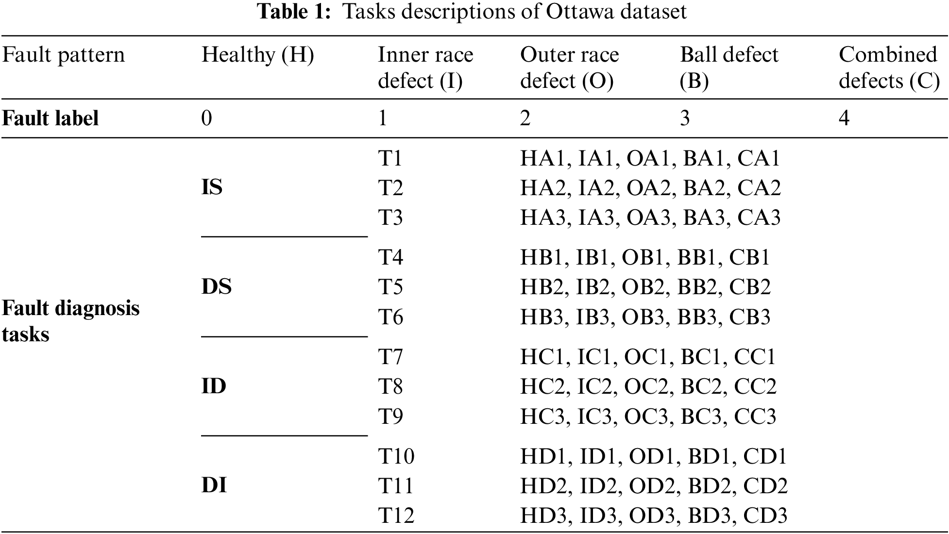
Ottawa bearing data [24] was obtained from a single sensor under time-varying speed conditions. Two ER16K ball bearings are installed, and one of them is used for bearing fault simulation experiments. The health conditions of the bearing include (1) healthy, (2) faulty with an inner race defect, (3) faulty with an outer race defect, (4) faulty with a ball defect, and (5) faulty with combined defects on the inner race, the outer race and a ball (Serial number Corresponding to sample labels 0–4).

All these data are sampled at 200 kHz and the sampling duration is 10 s. The Ottawa dataset contains four variable speed conditions: (i) Increasing speed (IS); (ii) Decreasing speed (DS); (iii) Increasing then decreasing speed (ID); (iv) Decreasing then increasing speed (DI).

Each variable speed condition has data files for three different speed fluctuation intervals. Details are shown in Table 1. Therefore, we construct 12 data domains Ot(n|n=03)(m|m=02) for experimental validation between different domains, where n denotes variable speed condition (i–iv) and m denotes three different speed fluctuation intervals. We sampled the raw data in overlap with a step size of 500, retaining 3000 normal samples and 1500 randomly selected fault samples. Random selection of fault samples can further satisfy the sample imbalance condition.

CLADAN training process in task T7_T12 (source = T7, target = T12) is shown in Fig. 5, where CL0, CL400, and CL800 indicate that 0, 400 and 800 true-labeled samples are input to the algorithm model, respectively. The rest of the training samples were labeled by CL, i.e., the proportion of true-labeled samples was set to 0, 10%, and 20%, respectively. After 100 epochs of training, the accuracy fluctuations of CLADAN in the source and target domains are shown in Fig. 5. As true-labeled samples increase, the fluctuation ranges of classifier accuracy decreases. When the proportion of real samples is low, maintaining model accuracy becomes challenging at a steady state. This phenomenon indicates that the adversarial learning process is not stable enough due to insufficient true-labeled samples. Besides, CLADAN still maintains some performance with a final convergence accuracy of 60% when true-labeled samples are not available. Fig. 6 visualizes the output distribution for the unlabeled samples in the target domain.

Figure 5: CLADAN training process in task T7_T12 (a) source (b) target

Figure 6: Visualization of target domain features in task T7_T12

The full comparative results of the experiment are shown in Fig. 7, and accuracy values are derived from the average accuracy of the last 10 epochs of the training process. By analysis, the performance of discrepancy-based DA is significantly weaker than that of adversarial-based DA under weakly-supervised conditions. CL contain limited information content such that domain confusion methods based on distance metrics are hard to blur the boundary sufficiently between the source and target domains. Adversarial-based DA reinforces the mutually exclusive role of complementary labels by deceiving domain discriminators. In addition, the performance of domain adaptation is further enhanced by assigning different weight coefficients to different weakly supervised samples by entropy conditions in CLADAN and CDAN. During the adversarial process, MDD executes domain alignment from the feature space rather than the original data space, realizing the learning of domain invariant features. It was found that while MDD also mitigates the disturbance of time-varying speed fluctuations, it leads to delayed convergence of the training process. In Fig. 7b, CLADAN consistently demonstrates excellent diagnostic capability in target domain under different data conditions. The accuracy of CLADAN is still not high enough in the absence of sufficient true-labeled samples due to the model cannot be trained sufficiently by CL samples with insufficient information. Based on the above results a reasonable hypothesis can be made that when the sample length increased or the number of sensor channels increased, the information content per unit time corresponding to CL will be expanded.

Figure 7: Accuracy comparisons in Ottawa (a) radar diagram in CL400. (b) Task T7_T12

3.2 HFXZ-I Wind Power System Simulation Experimental Platform

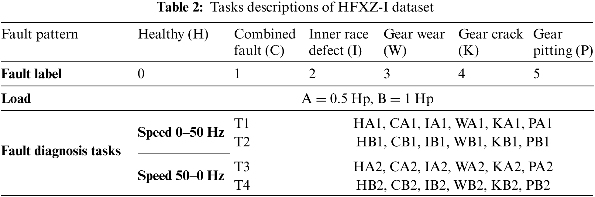
The development of wind power systems is in line with the current international trend of “reducing carbon emissions, achieving carbon neutrality”. The HFXZ-I in Fig. 8 is currently a simulation experiment platform for common wind power transmission systems. The relevant basic parameters are shown in Table 2. We obtained 11 channels and 4 channels of raw data on the planetary gearbox and helical gearbox, respectively, where two three-axis acceleration sensors were installed on the planetary gearbox to obtain the dynamic response in different vibration directions. All these data are sampled at 10.24 kHz and the sampling duration is 60 s. The gearbox health status details and task details are shown in Table 2. We set four variable speed conditions: (i) Decreasing speed 50–0 Hz, 0.5 HP (ii) Increasing speed 0–50 Hz, 0.5 HP (iii) Decreasing speed 50–0 Hz, 1 HP (iv) Increasing speed 0–50 Hz, 1HP. The data step size of overlapping sampling is 500. We obtained four data domains, each containing 2000 normal samples and 1000 faulty samples. We have fewer samples compared to Ottawa bearing experiments, but each sample has more abundant information due to the additional monitoring channels.

Figure 8: HFXZ-I wind gearbox experiment platform

CLADAN training process in task T2_T1 (source = T2, target = T1) is shown in Fig. 9, where CL0, CL200, CL400 indicate that 0, 200 and 400 true-labeled samples are input to the algorithm model, respectively. The proportion of true-labeled samples in the source domain still satisfies the dataset construction condition. Meanwhile, some of the fault types being set, such as gear wear, have much weaker signal feedback due to the minor degree of the fault, meaning that the learning process of the model is more difficult. After 100 epochs of training, the accuracy fluctuations of CLADAN in the source and target domains are shown in Fig. 9. It can be found that when the proportion of true-labeled samples reaches 10% (i.e., CL200), the training accuracy of the source domain is already close to CL400 (20% true-labeled samples). Compared with Ottawa bearing experiments, the target domain’s overall accuracy also has a significant improvement, while the accuracy fluctuation tends to moderate. This suggests that as the amount of information in true-labeled data increases, CL learning performs better and CLADAN is more stable. Fig. 10 visualizes the output distribution for the unlabeled samples from HFXZ-I dataset in the task T2_T1 target domain. It can be intuitively seen that the inter-class distance in the target domain is amplified and the intra-class distance is reduced. This suggests that CL learning that fuse multiple sources of information are able to retain a greater amount of information, guiding CLADAN to better identify unlabeled fault samples under weakly supervised conditions. All fault diagnosis comparison experiments are shown in Fig. 11. The model performance improves significantly at CL200.

Figure 9: CLADAN training process in task T2_T1 (a) source (b) target

Figure 10: Visualization of target domain features in task T2_T1

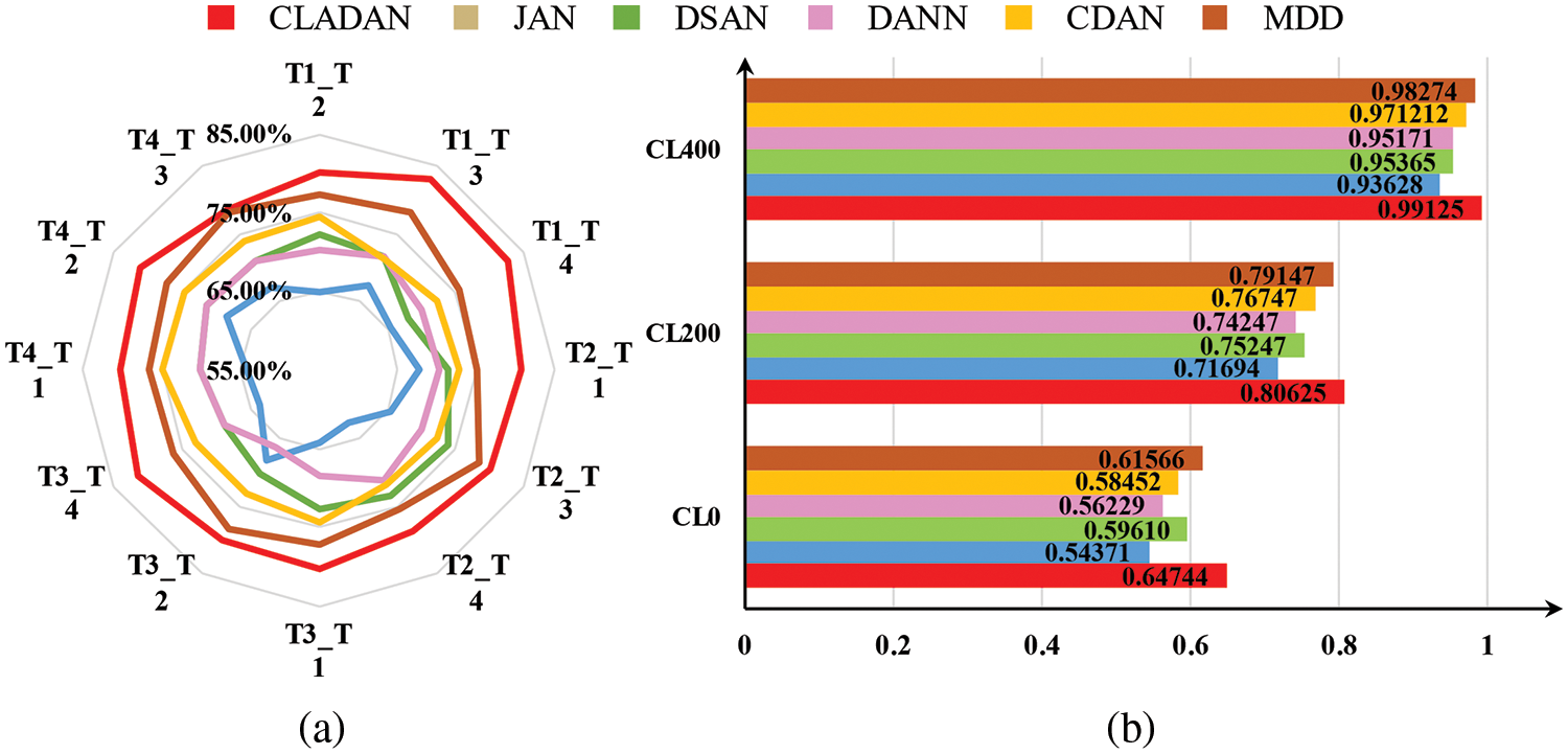
Figure 11: Accuracy comparisons in HFXZ-I (a) radar diagram in CL200. (b) Task T2_T1

3.3 VAR Ablation Study and Parameter Optimization

In this subsection, we conduct ablation experiments to show the contribution of the different components in CLADAN. In particular, it is necessary to further verify the immunity of the VAR to speed fluctuations. Since VAR is implicit in the training process, it is thus difficult to interpret its suppression of time-varying speed intuitively from a signal perspective. However, external conditions, such as time-varying rotational speeds, can lead to reduced generalization of cross- domain diagnostic models, while it is undoubtedly true that adding local perturbations to adversarial training can enhance model generalization. Therefore, we reasonably believe that VAR will improve the robustness of the model and thus suppress the time-varying speed disturbance implicitly. DANN and CDAN can be considered as two sets of ablation experiments. Based on the gearbox experimental data CL400, we consider following baselines: (1) DANN: Train CLADAN without conditioning and VAR, namely train domain discriminator Gd only based on the output features of Gf, VAR and the predicted outer product of Gy do not participate in training. (2) CDAN: Train CLADAN without VAR. (3) WO/D: Train CLADAN without the discretizing category probabilities in Eq. (11). The results of the ablation experiment are shown on the left in Fig. 12. It can be found that adding conditional distributions on the input side captures the multimodal structures of distributions with cross-covariance dependency between the features and classes, improving transfer learning performance significantly. Comparing CLADAN with WO/D was able to demonstrate that discretizing category probabilities has a positive effect on domain adversarial training for the CL dataset. Discretizing category probabilities can sharpen the representation of conditional probabilities when CL is used as an input to the conditional distribution. While CLADAN’s performance is not guaranteed to be optimal at all times during transfer tasks, its overall fault diagnosis performance is still superior. In addition, we perform an optimization search for the key parameters in Eq. (13) with results in Fig. 12 right. It can be observed that CLADAN performs best for α=0.3 and λ=1.2.

Figure 12: Results of ablation study and parameter optimization

Current DA-based fault diagnosis techniques often require high-quality and sufficient source-domain labeled data. However, a large number of data samples with pending labels in the industrial field are is unavailable for direct training, resulting in the underutilization of these feature-rich data resources. Hence, the CL-based weakly supervised learning approach can be employed to assign fuzzy conceptual labels to these data samples. Meanwhile, CL differs from traditional pseudo-labeling methods in that its annotation process leverages a priori knowledge, yet its annotation cost is less than that of labeling real samples. The efficacy of DA relies not on labels but on generalizing the generalized feature extraction patterns by capturing the underlying structure of the training data. Thus, in domain-adversarial training, injecting random perturbations into the target domain can also substantially improve the robustness of the cross-domain fault diagnosis model, leading to better learning of domain-invariant features under time-varying rotational speed conditions and implicitly removing the interference of fault-irrelevant components in the data content.

4  Conclusions

In this paper, CLADAN is developed for typical non-ideal scenarios of industrial sites. We integrate time-varying rotational speed conditions and weakly supervised learning conditions into cross-domain fault diagnosis, and use budget-friendly complementary labels to annotate unlabeled data in the source domain. In experiments, we establish a series of demanding conditions and complex faults to simulate industrial scenarios and we obtain accurate diagnostic results with CLADAN. The subsequent steps will delve into domain adaptation techniques for multiple CLs of the same sample, enhancing the learning performance of CL0, (3) Alternative solutions for time-varying speed conditions.

Acknowledgement: The authors wish to express their appreciation to the reviewers for their helpful suggestions which greatly improved the presentation of this paper.

Funding Statement: This work is supported by Shanxi Scholarship Council of China (2022-141) and Fundamental Research Program of Shanxi Province (202203021211096).

Author Contributions: The authors confirm contribution to the paper as follows: Study conception and design: Liu S., Wang Y. and Huang J.; methodology: Liu S.; software: Liu S.; validation: Liu S., Huang J. and Ma J.; formal analysis: Liu S.; investigation: Jing L.; resources: Ma J.; data curation: Liu S.; writing—original draft preparation: Liu S.; writing—review and editing: Liu S.; visualization: Liu S.; supervision: Huang J.; project administration: Huang J.; funding acquisition: Huang J. and Liu S. All authors have read and agreed to the published version of the manuscript.

Availability of Data and Materials: Data available on request from the authors. The data that support the findings of this study are available from the corresponding author upon reasonable request.

Conflicts of Interest: The authors declare that they have no conflicts of interest to report regarding the present study.

References

1. X. Chen, G. Shu, K. Zhang, M. Duan, and L. Li, “A fault characteristics extraction method for rolling bearing with variable rotational speed using adaptive time-varying comb filtering and order tracking,” J. Mech. Sci. Technol., vol. 36, no. 3, pp. 1171–1182, Mar. 2022. doi: 10.1007/s12206-022-0209-4. [Google Scholar] [CrossRef]

2. J. Yang, C. Yang, X. Zhuang, H. Liu, and Z. Wang, “Unknown bearing fault diagnosis under time-varying speed conditions and strong noise background,” Nonlinear Dyn., vol. 107, no. 3, pp. 2177–2193, Feb. 2022. doi: 10.1007/s11071-021-07078-8. [Google Scholar] [CrossRef]

3. F. Hou, I. Selesnick, J. Chen, and G. Dong, “Fault diagnosis for rolling bearings under unknown time-varying speed conditions with sparse representation,” J. Sound Vib., vol. 494, pp. 115854, Mar. 2021. doi: 10.1016/j.jsv.2020.115854. [Google Scholar] [CrossRef]

4. B. Han, G. Zhang, J. Wang, X. Wang, S. Jia and J. He, “Research and application of regularized sparse filtering model for intelligent fault diagnosis under large speed fluctuation,” IEEE Access, vol. 8, pp. 39809–39818, 2020. doi: 10.1109/ACCESS.2020.2975531. [Google Scholar] [CrossRef]

5. W. Huang, J. Cheng, and Y. Yang, “Rolling bearing fault diagnosis and performance degradation assessment under variable operation conditions based on nuisance attribute projection,” Mech. Syst. Signal Process., vol. 114, pp. 165–188, 2019. doi: 10.1016/j.ymssp.2018.05.015. [Google Scholar] [CrossRef]

6. S. Yan, H. Shao, Y. Xiao, J. Zhou, Y. Xu and J. Wan, “Semi-supervised fault diagnosis of machinery using LPS-DGAT under speed fluctuation and extremely low labeled rates,” Adv. Eng. Inform., vol. 53, pp. 101648, Aug. 2022. doi: 10.1016/j.aei.2022.101648. [Google Scholar] [CrossRef]

7. T. Han, C. Liu, W. Yang, and D. Jiang, “Deep transfer network with joint distribution adaptation: A new intelligent fault diagnosis framework for industry application,” ISA Trans., vol. 97, pp. 269–281, Feb. 2020. doi: 10.1016/j.isatra.2019.08.012. [Google Scholar] [PubMed] [CrossRef]

8. G. Wilson and D. J. Cook, “A survey of unsupervised deep domain adaptation,” ACM Trans. Intell. Syst. Technol., vol. 11, no. 5, pp. 1–46, Jul. 2020. doi: 10.1145/3400066. [Google Scholar] [PubMed] [CrossRef]

9. Z. Fang, J. Lu, F. Liu, J. Xuan, and G. Zhang, “Open set domain adaptation: Theoretical bound and algorithm,” IEEE Trans. Neural Netw. Learn. Syst., vol. 32, no. 10, pp. 4309–4322, Oct. 2021. doi: 10.1109/TNNLS.2020.3017213. [Google Scholar] [PubMed] [CrossRef]

10. M. Long, H. Zhu, J. Wang, and M. I. Jordan, “Deep transfer learning with joint adaptation networks,” in Proc. 34th Int. Conf. Mach. Learn., vol. 70, 2017, pp. 2208–2217. [Google Scholar]

11. Y. Zhu et al., “Deep subdomain adaptation network for image classification,” IEEE Trans. Neural Netw. Learn. Syst., vol. 32, no. 4, pp. 1713–1722, Apr. 2021. doi: 10.1109/TNNLS.2020.2988928. [Google Scholar] [PubMed] [CrossRef]

12. J. Luo, J. Huang, and H. Li, “A case study of conditional deep convolutional generative adversarial networks in machine fault diagnosis,” J. Intell. Manuf., vol. 32, no. 2, pp. 407–425, Feb. 2021. doi: 10.1007/s10845-020-01579-w. [Google Scholar] [CrossRef]

13. Y. Ganin et al., “Domain-adversarial training of neural networks,” in G. Csurka (Ed.Domain Adaptation in Computer Vision Applications, Cham: Springer International Publishing, 2017, pp. 189–209. doi: 10.1007/978-3-319-58347-1_10. [Google Scholar] [CrossRef]

14. M. Long, Z. Cao, J. Wang, and M. I. Jordan, “Conditional adversarial domain adaptation,” 2018. doi: 10.48550/arXiv.1705.10667. [Google Scholar] [CrossRef]

15. J. Li, E. Chen, Z. Ding, L. Zhu, K. Lu and H. T. Shen, “Maximum density divergence for domain adaptation,” IEEE Trans. Pattern Anal. Mach. Intell., vol. 43, no. 11, pp. 3918–3930, Nov. 2021. doi: 10.1109/TPAMI.2020.2991050. [Google Scholar] [PubMed] [CrossRef]

16. Y. Qin, Q. Yao, Y. Wang, and Y. Mao, “Parameter sharing adversarial domain adaptation networks for fault transfer diagnosis of planetary gearboxes,” Mech. Syst. Signal Process., vol. 160, pp. 107936, Nov. 2021. doi: 10.1016/j.ymssp.2021.107936. [Google Scholar] [CrossRef]

17. Y. Dong, Y. Li, H. Zheng, R. Wang, and M. Xu, “A new dynamic model and transfer learning based intelligent fault diagnosis framework for rolling element bearings race faults: Solving the small sample problem,” ISA Trans., vol. 121, pp. 327–348, Feb. 2022. doi: 10.1016/j.isatra.2021.03.042. [Google Scholar] [PubMed] [CrossRef]

18. T. Ishida, G. Niu, W. Hu, and M. Sugiyama, “Learning from complementary labels,” 2017. doi: 10.48550/arXiv.1705.07541. [Google Scholar] [CrossRef]

19. T. Ishida, G. Niu, A. K. Menon, and M. Sugiyama, “Complementary-label learning for arbitrary losses and models,” 2018. doi: 10.48550/ARXIV.1810.04327. [Google Scholar] [CrossRef]

20. T. Miyato, S. Maeda, M. Koyama, K. Nakae, and S. Ishii, “Distributional smoothing with virtual adversarial training,” 2015. doi: 10.48550/ARXIV.1507.00677. [Google Scholar] [CrossRef]

21. T. Miyato, S. I. Maeda, M. Koyama, and S. Ishii, “Virtual adversarial training: A regularization method for supervised and semi-supervised learning,” IEEE Trans. Pattern Anal. Mach. Intell., vol. 41, no. 8, pp. 1979–1993, Aug. 2019. doi: 10.1109/TPAMI.2018.2858821. [Google Scholar] [PubMed] [CrossRef]

22. Y. Shu, Z. Cao, M. Long, and J. Wang, “Transferable curriculum for weakly-supervised domain adaptation,” in Proc. of the AAAI Conf. on Artif. Intell., AAAI Press, vol. 33, no. 1, 2019. doi: 10.1609/aaai.v33i01.33014951. [Google Scholar] [CrossRef]

23. Y. Zhang, F. Liu, Z. Fang, B. Yuan, G. Zhang and J. Lu, “Clarinet: A one-step approach towards budget-friendly unsupervised domain adaptation,” in C. Bessiere (Ed.Proc. Twenty-Ninth Int. Joint Conf. on Artificial Intell., Jul. 2020, pp. 2526–2532. doi: 10.24963/ijcai.2020/350. [Google Scholar] [CrossRef]

24. H. Huang and N. Baddour, “Bearing vibration data collected under time-varying rotational speed conditions,” Data Brief, vol. 21, pp. 1745–1749, Dec. 2018. doi: 10.1016/j.dib.2018.11.019. [Google Scholar] [PubMed] [CrossRef]