Contribution Tracking Feature Selection (CTFS) Based on the Fusion of Sparse Autoencoder and Mutual Information

1  Introduction

With the rapid development of information technology, data mining, image processing, bioinformatics, and other fields have generated massive and high-dimensional data. High-dimensional datasets dramatically increase the algorithm’s demands in terms of time and space [1], and there is a side effect on the efficiency or effectiveness of the learning system. Moreover, for some learning tasks, such as classification and regression, computational analysis is feasible in low-dimensional space but becomes very difficult in high-dimensional space. To address this problem, one can use either feature extraction or feature selection, two standard dimensionality reduction methods. Feature extraction generally utilizes linear and nonlinear mapping to obtain low-dimensional features. However, for some specific issues, such as genomic datasets, this method may overlook the inherent physical properties of the original genes. Feature selection, also called attribute subset selection [2,3], aims to minimize the dimensionality of the feature set while approaching, maintaining, or even improving the accuracy of the classification model compared to the entire feature set. In addition, feature selection removes irrelevant and redundant features, improving the model’s generalization ability while avoiding dimensionality catastrophe [4,5].

Feature selection is commonly viewed as a combinatorial optimization problem, mainly involving deciding whether to include each feature from the entire feature set. For a dataset with m features, an exhaustive search algorithm requires 2m−1 iterations, representing a non-trivial task categorized as the NP-Hard problem [6]. Over the past few years, due to the widespread application of some effective deep neural networks and classification algorithms [7,8], feature selection has become a hot topic in this field.

In general, existing supervised and unsupervised feature selection methods can be classified as filter methods [9–12], wrapper methods [13–15], and embedded methods [7,16,17]. Moreover, researchers have attempted to achieve higher classification performance by putting meta-heuristic algorithms into the feature selection problem to search for optimal or near-optimal feature subsets [18], which serve as a wrapper method for addressing the feature selection problem by necessitating a classifier’s specification to assess the solution’s quality.

A notable concern in feature selection revolves around selecting features from large sets of high-dimensional datasets. This challenge remains for meta-heuristic algorithms due to their inherent limitations in attaining optimal solutions within a restricted time. Therefore, an applicable and efficient meta-heuristic algorithm must address the feature selection problem with fewer evaluations, higher accuracy, and faster speed. In addition, few studies have simultaneously explored the impact of individual features on the overall performance of a feature subset and non-linear relationships between features. There is a lack of related research on whether this impact helps the heuristic algorithm efficiently discover the optimal feature subset. Based on the above analysis, this paper proposes a novel approach called CTFS. The primary contributions of this paper are outlined below:

•   We employ an unsupervised learning methodology, utilizing an autoencoder network to unveil non-linear relationships between features. Consequently, this approach alleviates missing label information and errors in classification results.

•   We adopt the deep learning structure to reduce the extra time and algorithmic complexity for the subsequent wrapper, making it more efficient and less computationally demanding.

•   Based on the autoencoder network, sparse training is incorporated to expedite network training and diminish memory occupation.

•   Integrating the feature contribution obtained from the network training in the first stage with the relationship between features and labels, a contribution tracking approach is proposed to find the optimal or near-optimal feature subset efficiently.

The subsequent sections of this paper are organized as follows. Section 2 describes the meta-heuristic algorithm based on the wrapper method and related works on the sparse autoencoder network. Section 3 thoroughly introduces the framework of the sparse autoencoder network. Section 4 proposes a novel wrapper feature selection method based on a contribution tracking mechanism. Computational comparison experiments of the proposed algorithm will be reported in Section 5. The last section will conclude the works of this paper and give the subsequent schemes in the research.

2  Related Work

The feature selection process consists of four main components: subset generation, subset evaluation, stopping criteria, and result validation. The method proposed in this paper is a wrapper-based technique, so filter-based and embedded feature selection methods are not part of the work in this paper. Different feature selection problems in many domains can be solved using meta-heuristic algorithms based on wrapper methods [19–22]. The following is a review of some of the metaheuristics that have been categorized according to the class of algorithms used, and several of the metaheuristics have been used in comparative experiments with our proposed algorithm. In addition, the research in this paper is related to autoencoder networks and sparse training, and an overview of deep neural network methods for feature selection problems is also presented at the end of the section.

PSO algorithms are conceptually simple, easy to implement, and have fast convergence; many PSO-based algorithms have been used for feature selection problems. A novel PSO-based feature selection approach was designed in [23], which can improve the population’s quality at each generation to jump out of the local optimum to some extent. The proposed method was combined with the filter Relief algorithm to get the weights of each feature and generate more optimal solutions. In addition, an agent model was used to select the best solution regarding diversity and convergence. Moreover, feature selection based on evolutionary multitasking is also a very hot topic. Wang et al. [24] proposed a novel PSO-based multi-task framework to achieve the information shared, which divided the initial population into two subpopulations. Extensive experiments showed the strong competitiveness of the approach compared with other algorithms. An effective FS method based on the idea of multitasking with knowledge transfer between different search space was developed in [25] on high-dimensional data. In addition, promising features were distinguished by a knee point selection scheme, and a novel variable-range strategy effectively reduced the search space of the population.

Harris Hawk optimization is a newly introduced swarm intelligence optimizer that can be used to solve a variety of combinatorial optimization problems. Peng et al. [26] improved the Harris Hawk algorithm by using a hierarchical mechanism that speeded up its operation without increasing its complexity, allowing the algorithm a shorter time and higher accuracy. Two limitations of Harris Hawk optimization were addressed in [27] by introducing chaotic dyadic in the initial stage to improve the population diversity of search agents. Then, a simulated annealing strategy was introduced in each iteration to reduce the risk of falling into a local optimum. Finally, the algorithm was applied to the feature selection problem, and experimental results on some tumor datasets demonstrated the superiority of the algorithm.

In addition to the two aforementioned optimization paradigms, various feature selection problems have been solved using other meta-heuristic algorithms. A modified binary Gray Wolf algorithm with two-stage mutation was developed in [28]. The two-phase mutation enhanced the exploitation capability of the algorithm. The experimental results showed the validity of the algorithm and good performance. Zhou et al. [29] proposed a genetic algorithm combining the correlation between feature-to-feature and feature-to-label, and the algorithm reduced the generation of poor solutions and improved the efficiency of the evolutionary process by utilizing correlations to guide the improvement of the crossover and mutation operators in the genetic algorithms. The algorithm was demonstrated to have good classification accuracy on four artificial datasets and six real datasets.

The main limitation of the aforementioned current wrapper methods is that their score function depends on training and predicting at least one model per iteration. Thus, this approach has a high computational cost. Also, wrappers are classifier-specific. Therefore, they may not obtain satisfactory results if the resulting selection is used with different classifiers other than the one used in training and become very prone to overfit.

On high-dimensional datasets, some fully connected layers of deep neural networks can prominently slow down the training speed and cause too much memory usage. Because of this, Han et al. [30] utilized a three-step method to prune redundant connections and achieved sparsity of weights by learning significant connections without degrading accuracy. Inspired by network science, Mocanu et al. [31] proposed a SET algorithm, which first introduced an Erdös-Rényi random graph to initialize the layer-to-layer connections between neurons. A dynamic updating approach was used to increase the generalizability of this structure in the network, and to prove its effectiveness, the article went on to perform supervised and unsupervised learning with different neural networks on multiple datasets. Atashgahi et al. [32] built on the approach of Han et al. [30] and used it for an unsupervised feature selection problem to achieve an optimal trade-off between classification and clustering accuracy, runtime, and maximum memory usage.

Given that the stochastic exploration of sparse topology requires more cycles in the drop-and-grow session [31], Sokar et al. [33] improved the drop-and-grow session. Work was put into the regrowth of the new connections. In this paper, we have improved on the work of Sokar et al. [33] by adjusting its input part. Meanwhile, connections in the input or output layer are re-estimated only by corresponding magnitudes during the drop operation.

3  Sparse Autoencoder

The autoencoder network employing sparse training is designed to capture the nonlinear relationships between features, which matters for our CTFS approach to quantitatively evaluate the contributions of individual features. In addition, it’s noteworthy that this mode of training the network can significantly reduce the runtime as well as the memory occupation [32].

3.1 Framework

3.1.1 Data Input

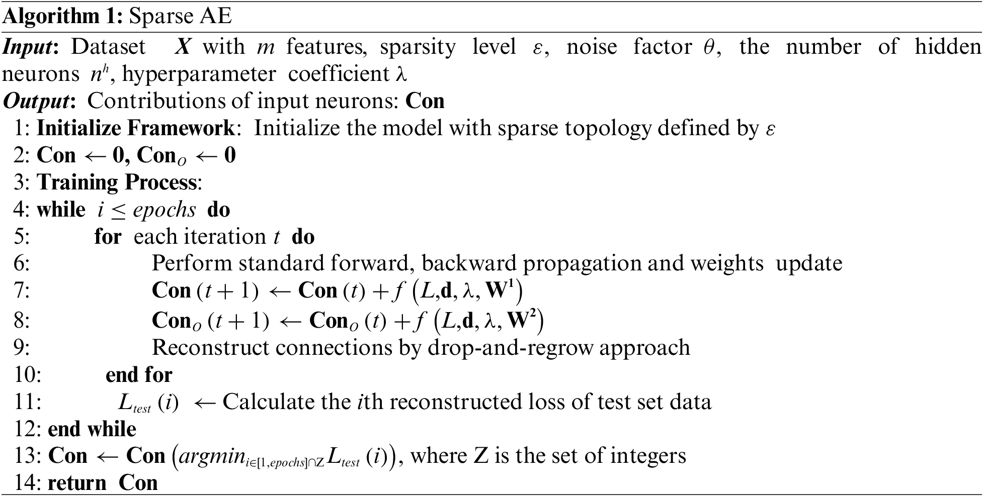
Assume a dataset with a sample size of n and dimension of m. The task is to obtain the contribution of each feature in the first stage. These contributions are used to report the importance level of each feature in the subsequent wrapper and prepare for the fusion of mutual information.

3.1.2 Initialization

Sparse Autoencoder (AE) is based on the structure of a neural network. Given the demands of short training time and low memory occupation, this paper adopts the model with the least hidden layer, using sparse connections instead of full ones. The sparse level ε of the network is obtained from Eq. (1):

ε=‖W1‖0m×nh(1)

Wl (l = 1, 2) is the sparse weight matrix of hidden layers, m is the number of features, and nh denotes the number of hidden layer neurons. The network is initialized with sparse weights uniformly distributed on the neurons.

3.1.3 Noise Input

To learn more robust features, Gaussian noise is added to perturb the original data:

x~=x+θ∗N(μ,σ2)(2)

In Eq. (2), x is the initial input vector from the dataset, θ denotes the noise factor that controls the level of corruption, and N(μ,σ2) is a Gaussian noise.

After obtaining the corrupted input, the autoencoder maps it to the latent representation e, followed by mapping e back to the reconstructed vector d. Here, the hidden representation e as well as the reconstructed vector d can be calculated from Eq. (3):

e=s(W1x~+b)d=s(W2e+b′)(3)

where s is the neuron activation function and b, b′ are the bias vectors of corresponding layer.

Next, the weight parameters are updated using a stochastic gradient descent algorithm, which minimizes the average reconstruction error:

LMSE=‖d−x‖22(4)

3.2 Training Process

Since the connections between initialized neurons are randomly generated, to enhance its generalizability, the improved SET approach proposed by Sokar et al. [33] is introduced here, and the overall structure of AE is depicted in Fig. 1. It proceeds as follows: after updating the weights using each batch of data, we adjust the sparse topology using the drop-and-regrow cycle. Given a score α, connections with less than the minimum level α are dropped from the sparse weight matrix Wl, and the same fraction of connections with weight 0 are regrown. This drop-and-regrow approach maintains the overall performance, which was described as well as proved by Han et al. [30].

Figure 1: Comprehensive overview of the sparse AE network. A sparse autoencoder is initialized with uniformly distributed sparse connections. During sparse training, the connections are redistributed in the most important neurons at iteration t during the “drop-and-regrow” cycle

Especially, new connections are not randomly regrown. Sokar et al. [33] gave a fast focus on new connections to informative features. The gradient of the loss concerning the output neuron ∂LMSE∂di is used to measure the sensitivity of the reconstruction error to the reconstructed output. Following that, we obtain Eq. (5), defining the contribution of the ith output neuron, denoted as (ConOi), at iteration t:

ConOi(t)=ConOi(t−1)+λ|∂LMSE∂di|+(1−λ)∑j=1nh|Wji2|(5)

Here (ConOi) is initially set to 0.Wji2 denotes the magnitude of the incoming connection between the jth hidden neuron and the ith output neuron. λ is a hyperparameter coefficient. Similarly, the same method is applied to the input neurons (Coni) by replacing the magnitude of output weights with input ones |W1|. This distributes the positions of the regrown new connections over these contributing neurons. This modified drop-and-regrow approach dynamically optimizes the sparse topology of the network, ultimately using (Coni) as the contribution of each input neuron. The pseudocode can be found in Algorithm 1:

4  Wrapper Feature Selection Using a Contribution Tracking Method

Wrapper feature selection methods usually specify a classifier, which evaluates the performance of a candidate feature subset by calculating the predicted values of the classification model. A large number of iterations are required to find the target feature subset that possesses the optimal performance when dealing with high-dimensional datasets. The computational time is considerable. Therefore, the primary task of the wrapper feature selection algorithm is to achieve a better balance between classification performance and running time.

The proposed algorithm employs a contribution tracking mechanism called CTFS, which fully considers these two indicators mentioned above. Specifically, the contribution of each feature incorporates the mutual information metrics from the filter method and the feature importance metrics from the AE network. Following that, a novel wrapper algorithm combining the feature contributions with its corresponding classification accuracy is given. Compared to the traditional wrapper methods, CTFS targets informative features through the contribution tracking strategy instead of finally reaching convergence through population-level evolution, and a classifier is necessary during the training time, which also varies from filter methods. The general framework of the proposed algorithm is illustrated in Fig. 2.

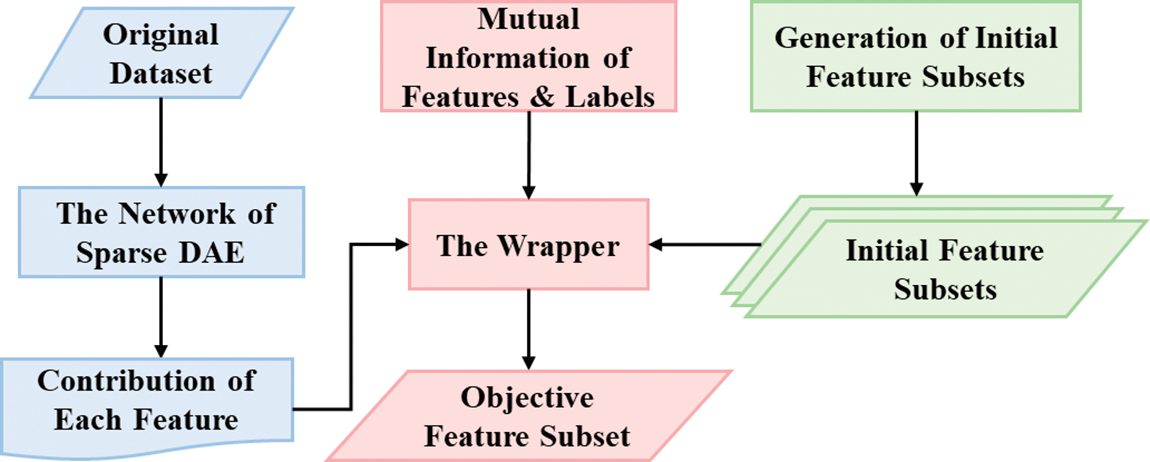
Figure 2: Flowchart of the proposed CTFS algorithm

4.1 Score Function

A score function is required to evaluate the merit of a candidate feature subset. In this paper, we use some performance metrics in the learning machine as its score function. The specific mathematical description is as follows:

Suppose there are m features in the original data, and one of the candidate feature subsets is represented by x=[x1,x2,…,xi,…,xm]. xi takes the value 0 or 1, which means whether the ith feature is selected or not. The best feature subset can be discovered by finding the highest score in the subset of candidate features, which can be denoted by the mathematical Eq. (6):

maxF(x)s.t.x=[x1,x2,…,xi,…,xm],xi∈{0,1}(6)

Here F(⋅) is related to the performance metrics of the classifier.

4.2 Generation of Initial Feature Subset

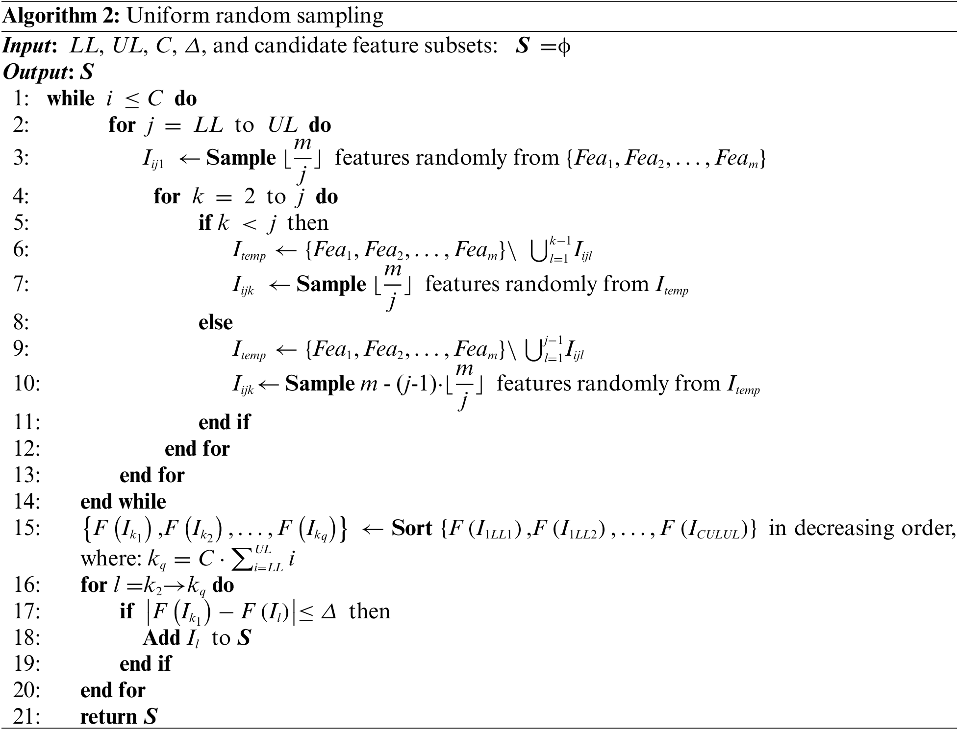
In this paper, many initial feature subsets are required for subsequent calculation. For some of the commonly used methods of generating initial feature subsets, such as the one-dimensional chaotic mapping method, taking into account that it is more sensitive to the initial conditions as well as the parameters, which will lead to a decrease in the uniformity and stochasticity of the sequences; in other words, each feature does not appear at the same frequency, and some features appear repeatedly in the subset while others never appear, which result in a negative influence on the acquisition of the target feature subset. This research develops a method to initialize the generation of the feature subset, which ensures that each feature has the same frequency of appearing in the initial randomly generated feature subset.

In Algorithm 2, the parameters LL and UL denote the upper and lower limits for dividing the set of features; the closer to the upper limit, the smaller the number of features in the initial feature subsets generated. C represents the number of repetitions. The parameter Δ is the tolerance for accepting poor initial feature subsets; when the classification accuracy of an initial feature subset differs too much from the best, then the corresponding initial feature subset will be deleted, and this parameter controls the number of initial feature subsets generated at the end.

4.3 Contribution Tracking Strategy

Current wrappers often do not adequately consider the influence of a single feature on the accuracy of a classification model. As a result, an improved wrapper feature selection algorithm has been developed to address this limitation, which is inspired by the fact that after obtaining the optimal or suboptimal feature subsets, we can know exactly which features work for classification accuracy. Accordingly, we will accumulate the dominance corresponding to the features that appear in the feature subsets with high classification accuracy. Given that unsupervised learning does not involve label information, this paper fuses the concept of mutual information to increase the information between features and labels.

We first introduce the concept of mutual information [10]. Suppose X and Y are two discrete random variables, and their mutual information MI(X;Y) can be defined as:

MI(X;Y)=∑y∈Y∑x∈Xp(x,y)log2(p(x,y)p(x)p(y))(7)

where p(x) is the marginal probability distribution function of X and p(x,y) is the joint probability distribution function of X and Y. We can find the relationship MIi between features and labels through the method above.

To facilitate the description, the symbol si is employed to indicate the joint action between the contribution (Coni) of the feature i and the relationship MIi with labels, as shown in Eq. (8):

si=Coni∗MIi(8)

Since the same feature in two different initial feature subsets shares an equal contribution, we adjust the original Eq. (8) to reflect the variations of the same feature in different feature subsets by introducing the target value F, that is:

si′(I)=si∗|lnF(I)|(9)

We quantitatively evaluate the possibility that subset I contains the feature i by thoroughly combining both the joint action si of the ith feature and the objective value of the feature subset. This formula also accounts for the fact that various candidate feature subsets share different si′ values for the same feature condition. That is to say, different candidate feature subsets affect the inclusion of feature i in the optimal feature subset.

Typically, if multiple local optimal solutions with good performance have been achieved, the optimal feature subsets will be easier to obtain after certain processing operations. The specific processing operations based on the contribution tracking method will be given subsequently.

This research generates quantities of initial feature subsets. For simplicity of description, suppose these subsets are I1,I2,…,Iq, respectively, then the probability of the feature i appearing in the jth subset is si′(Ij). The cumulative effect of feature i in the q candidate feature subsets can be obtained in Eq. (10):

Ci(I1→Iq)=∑j=1qsi′(Ij)(10)

where the symbol Ci is used to denote this cumulative effect, which is the aforementioned contribution tracking mechanism. Then, it is necessary to find a mean value for this cumulative impact, which is used to quantitatively characterize the probability of the feature i appearing in the target feature subset. Ci′ can be achieved by Eq. (11):

Ci′=Ci/Oi(11)

where Oi denotes the cumulative occurrences of feature i in q candidate feature subsets. From Eq. (11), we obtain the Ci′ of each feature in the target feature subset, but the number of features cannot be determined. To address this problem, we design a greedy approach. Initially, the dominance of the features is sorted in descending order, and then the features are added sequentially in descending feature order. Since the dimension of the original dataset is m, m additions in total are required. Every time a feature is added, the value of the corresponding objective function is calculated. Finally, we select the feature subset with the largest objective function value as the target one. The pseudocode for obtaining the target feature subset is shown in Algorithm 3:

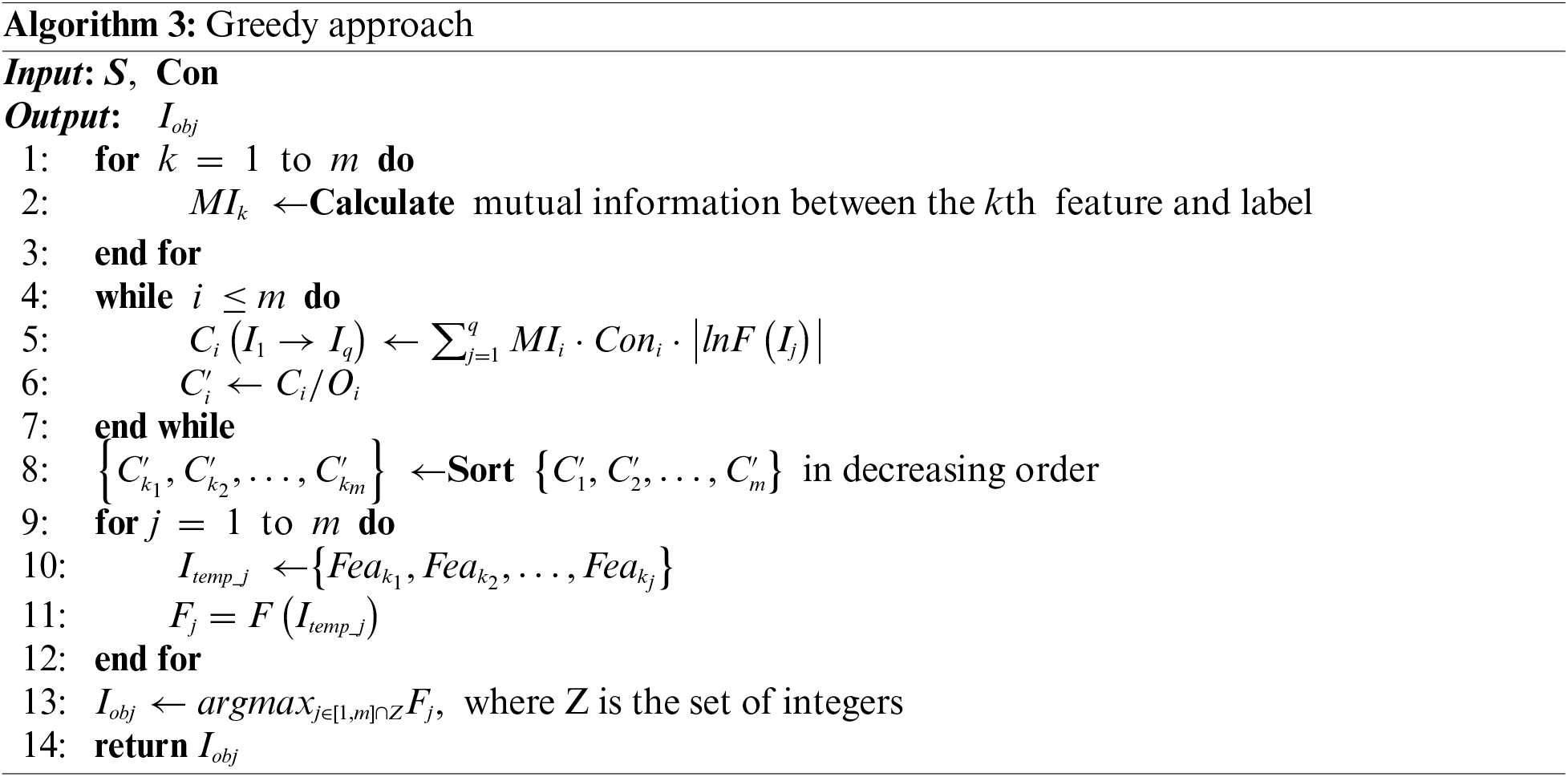
The objective feature subset is finally obtained through the above approach, and the overall framework structure of the proposed CTFS algorithm is depicted in Fig. 3.

Figure 3: Structure of the proposed CTFS algorithm

5  Experiments and Analysis

5.1 Test Datasets

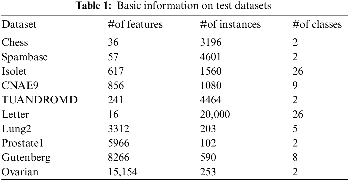
To verify the performance of the proposed algorithm, eight datasets from the UCI repository and two datasets from the literature [34] are selected. Given the huge amount of data in real life, the characteristics of the selected datasets are also large sample sizes and high dimensions. These datasets involve life, microarrays, computer science, business, and other fields. Table 1 lists their basic information: the name of datasets (Dataset), the number of features (#of features), the number of instances (#of instances), and the number of classes (#of classes).

5.2 Comparative Methods and Parameter Settings

The binary HHO, GWO, and PSO algorithms perform well in solving the feature selection problem. This research selects the following algorithms for comparison with the proposed CTFS algorithm: all available features (Full), the binary HHO (BHHO), the correlation-guided updating strategy and surrogate-assisted PSO (CUS-SPSO) [23], and the Grey-Wolf algorithm integrating a two-phase mutation (TMGWO) [28]. These comparison algorithms are re-programmed based on the algorithm flow and pseudocode in the literature.

To illustrate the generalizability of the algorithm and analyze the effect of the classifier on performance, this research selects two classifiers, KNN and Bayesian, where K is set to 5. For each dataset, 80% of the samples are used as training sets randomly, and the remaining 20% are selected as test sets. During the training process, k-fold cross-validation is employed, where k is set to 5. The specific procedure is to iteratively rotate the training and test sets k times in sequence. After the training, the selected features will be evaluated on the test set samples to obtain the corresponding accuracy, recall rate, and F1 score.

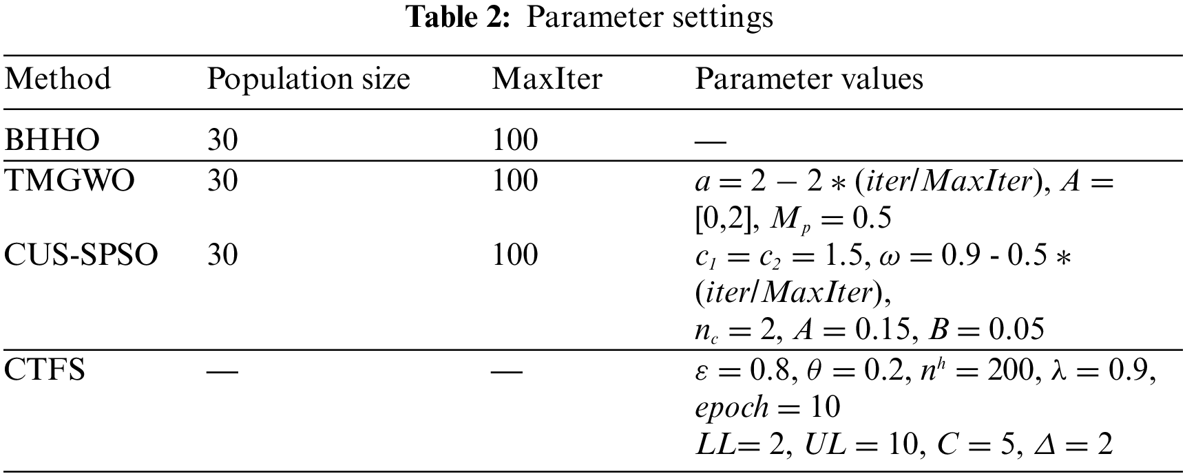
The parameters of the algorithms proposed in this paper, as well as the feature selection methods used for comparison, are given in Table 2. For the swarm intelligence algorithms, we set the maximum number of iterations to 100 and the population size to 30. The settings of other parameter values are adjusted according to the characteristics of each algorithm.

5.3 Results and Discussions

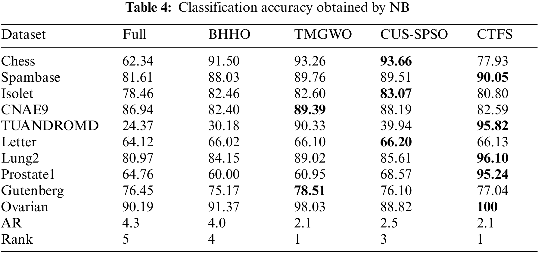
Tables 3 and 4 list the average classification accuracies of the proposed CTFS method and the other four comparison algorithms based on ten independent runs on the test sets. The epoch of the SAE network is also set to 10, which is a balance between the reconstruction error of the test set and the training time of the network. Moreover, the average rank approach is adopted to express the average ranking performance of the methods, which is denoted as AR.

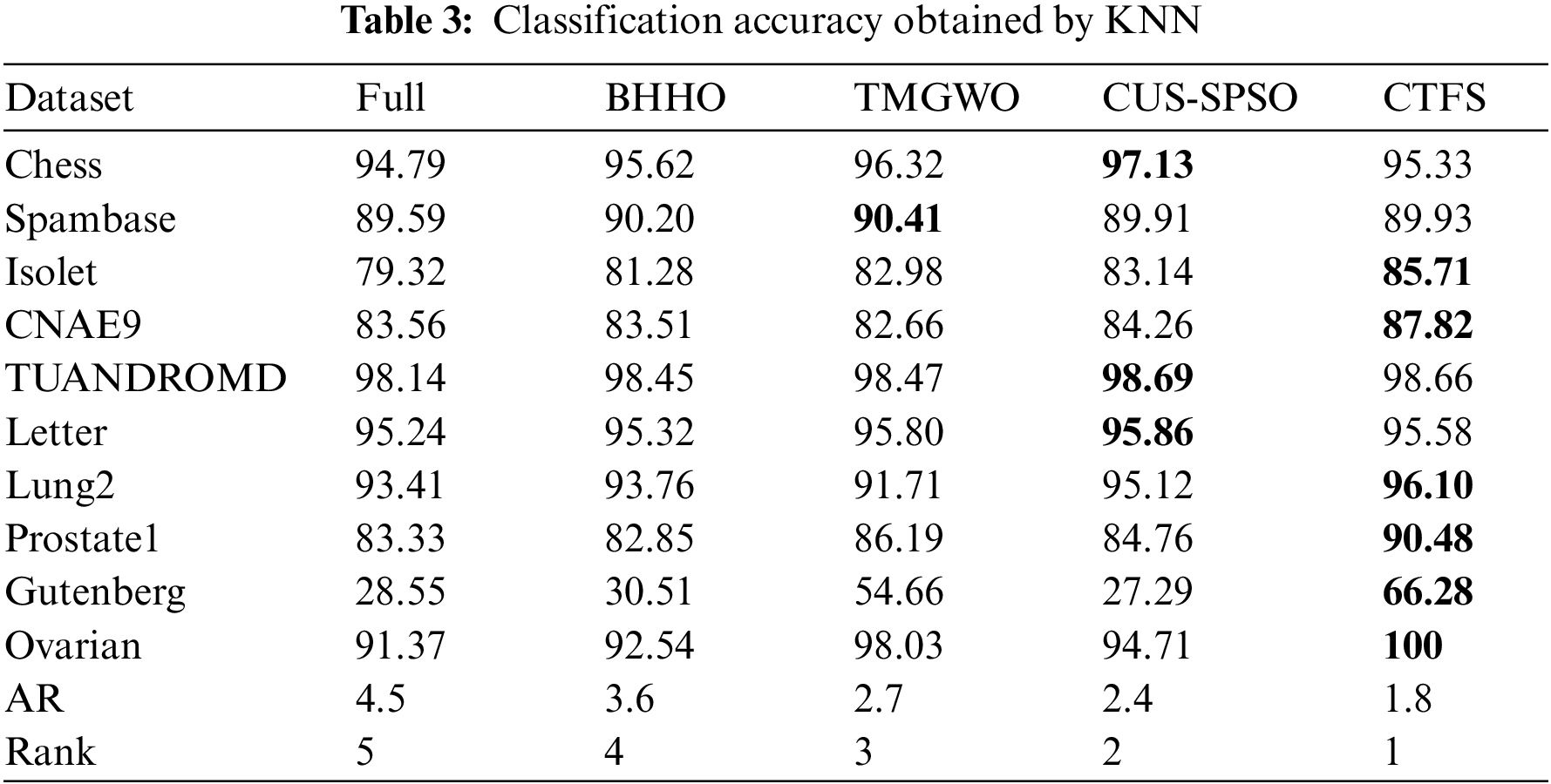
From Table 3, the CTFS algorithm shows better performance on multiple test datasets compared to other stochastic approaches when KNN is used as a classifier. Specifically, the CTFS method achieves the best classification accuracy on 6 out of 10 datasets with a large sample size and high dimensions. Meanwhile, for the remaining 4 test datasets, the relative errors between the classification accuracy obtained by the CTFS method and the highest acquired by other comparison algorithms range from a maximum of 1.8% to a minimum of 0.03%, which is a relatively small gap. Therefore, it is concluded that the CTFS algorithm has a prominent advantage over other compared wrapper algorithms in terms of classification accuracy when handling test datasets with large sample sizes and high dimensions.

Different from the KNN classifier, the performance of the CTFS algorithm varies with the Bayesian classifier. Table 4 demonstrates that the classification accuracy of the CTFS algorithm is worse than that of other comparison algorithms on the test datasets with large sample sizes and medium dimensions. However, for test datasets with a moderate sample size and high dimensions, such as Lung2, Prostate1, etc., the CTFS algorithm achieves the best classification accuracy.

From Tables 3 and 4, as the number of features in the dataset grows, the CTFS algorithm gradually demonstrates its capability to efficiently discern the objective feature sets. When the number of features in the test datasets reaches 15,154, the classification accuracy of the CTFS method is 100%, while the classification accuracies of the other four compared algorithms are 91.37%, 92.54%, 98.03%, and 94.71%, respectively.

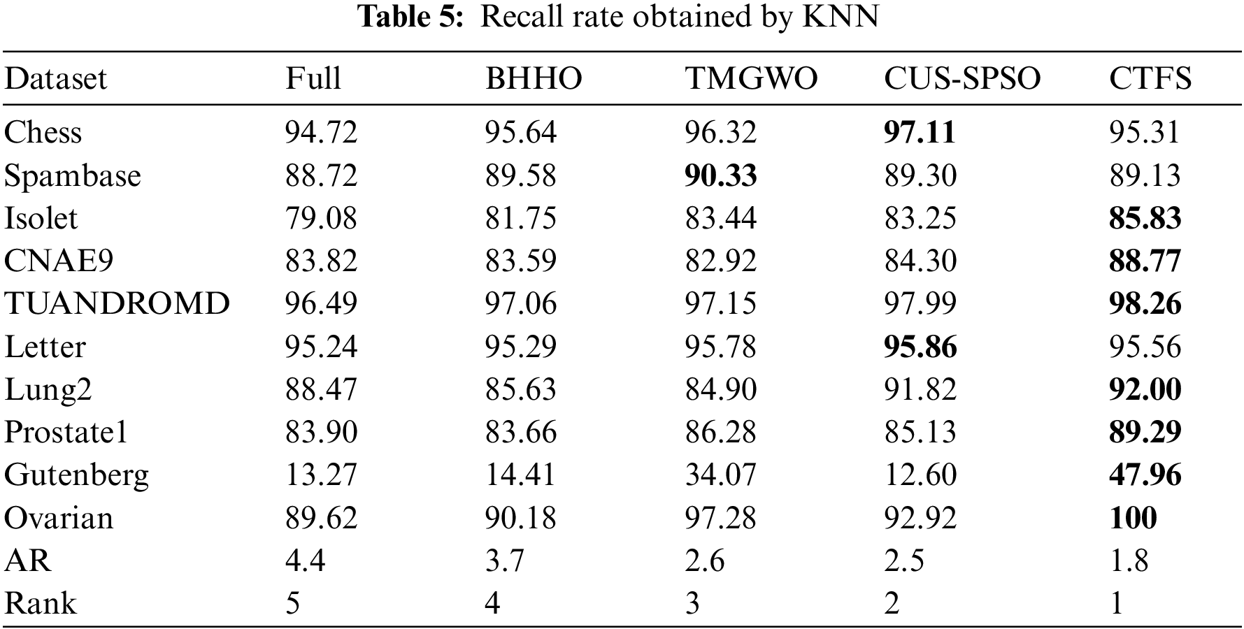
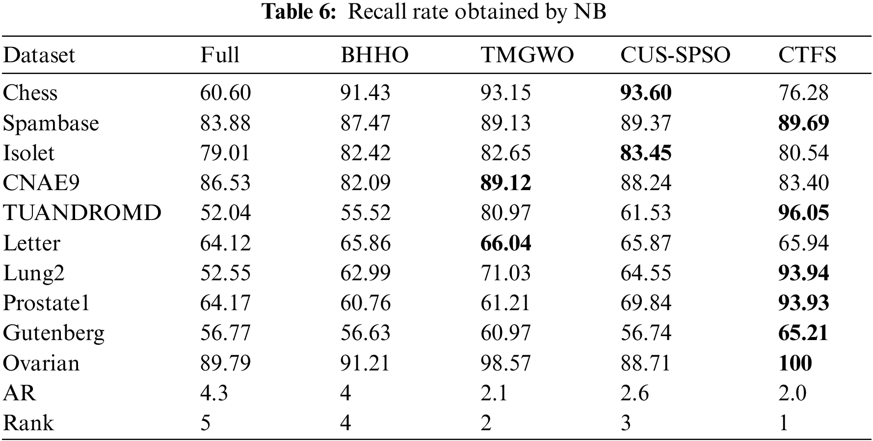
To evaluate the comprehensive classification performance of the proposed CTFS algorithm, we also analyze the recall rate and F1 score on various test datasets. Tables 5 and 6 record the recall rate using KNN and Bayesian as classifiers, respectively. From Table 5, the CTFS approach achieves a remarkable recall rate on 7 out of 10 datasets. Similarly, in Table 6, the CTFS algorithm obtains the highest recall rate on 6 out of all datasets with an average recall rate of 84.5%, while the TMGWO algorithm has an average recall rate of 79.28%, which still holds the highest value among the four comparison algorithms.

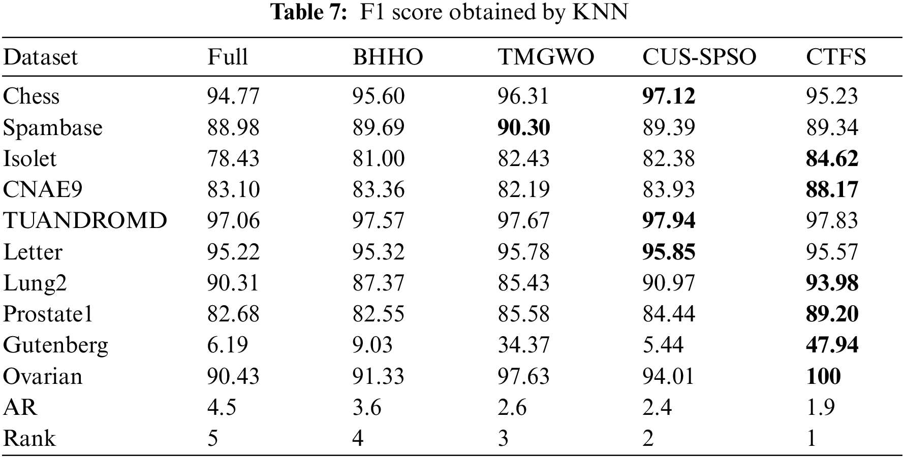
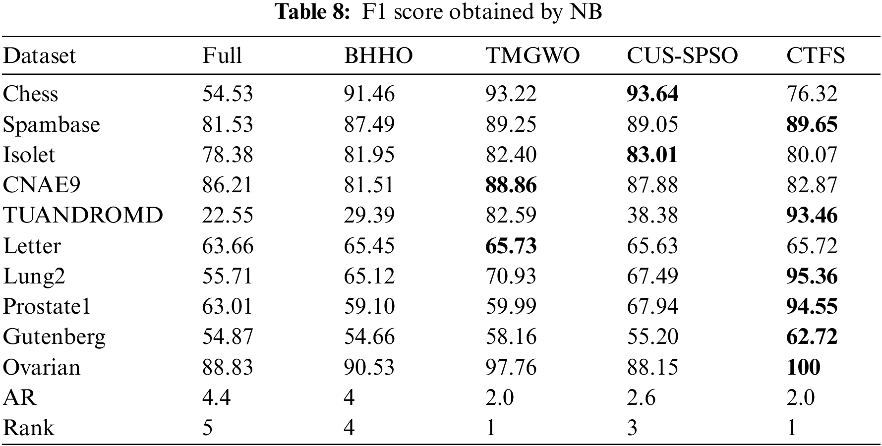
Tables 7 and 8 illustrate the F1 score on ten datasets using KNN and Bayesian as classifiers. From Table 7, the CTFS method achieves the highest F1 score on 6 out of 10 datasets. For the rest of the test datasets, the relative errors between the F1 score obtained by the CTFS method and the highest acquired by other comparison algorithms range from a maximum of 1.89% to a minimum of 0.14%, which is a relatively small difference. Table 8 shows the good performance of the CTFS algorithm using Bayesian as a classifier, which reaches the highest F1 score on 6 out of all test datasets with an average F1 score of 84.07%. From Tables 5–8, it can be summarized that, in addition to the classification accuracy metric, the CTFS algorithm still maintains prominent performance advantages.

In addition to the classification performance metrics, the number of selected features is also an important reference indicator. Generally, the lower the dimension of the candidate feature subset, the stronger its generalization performance and the better the dimensionality reduction effect of the algorithm. Table 9 shows the number of features selected by the five algorithms on each dataset. The CTFS algorithm achieves the minimum number of features when using KNN as a classifier on 8 out of all test datasets. Based on Tables 3–8, it is concluded that the CTFS algorithm can achieve remarkable classification performance with a relatively small number of features.

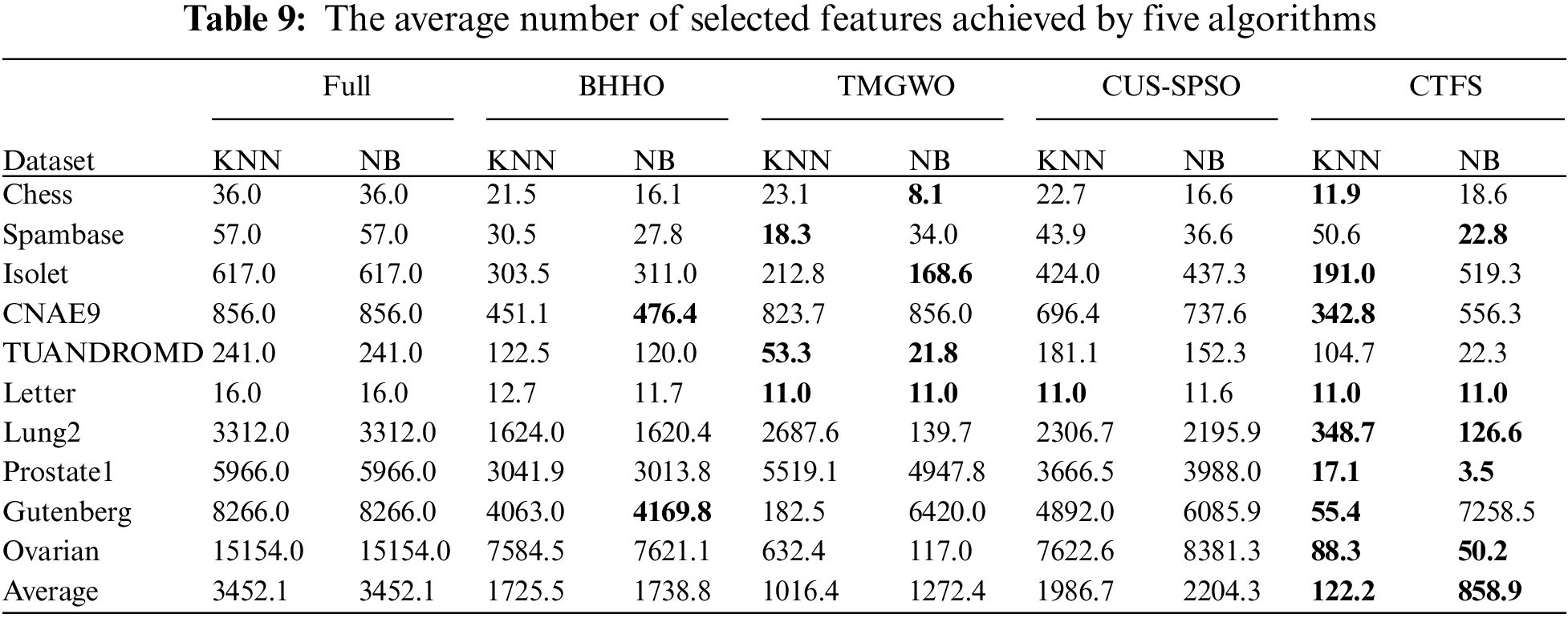
Fig. 4 shows the comparison of the number of selected features for four algorithms on ten test datasets. Specifically, we define μij=Nsij/Numi(i=1,2,…,10,j=2,3,4,5) to normalize the number of features selected by each algorithm, where i denotes the number of test datasets, and j is the sequence of the algorithms in the table. Nsij represents the number of features selected by the jth algorithm on the ith dataset. Numi is the number of the initial features on the ith dataset. In the spider web diagram, the red lines denote the CTFS algorithm. The red lines are distributed mostly inside the entire spider web, indicating that the CTFS algorithm selects the fewest features. The red lines are primarily at the center of the spider web on Prostate1 and Gutenberg when Bayesian is used as a classifier, which shows the extremely marked dimensionality reduction effect of the CTFS algorithm on these two datasets.

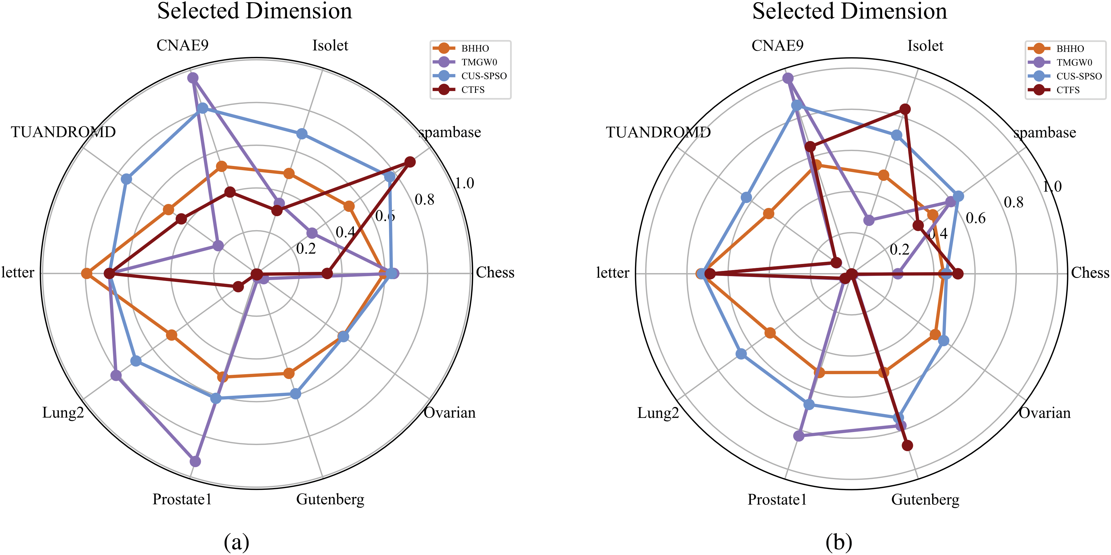
Figure 4: Number of selected features of different methods on ten datasets (a) KNN classifier (b) Bayesian classifier

Besides the indicators mentioned above to verify the efficiency of each method, running time is also another metric that cannot be ignored. The purpose of feature selection is to select key information attributes with less time and cost to achieve higher classification performance. Table 10 lists the average running time consumed by these algorithms. Compared with other comparison algorithms, the CTFS algorithm requires the least running time on most datasets.

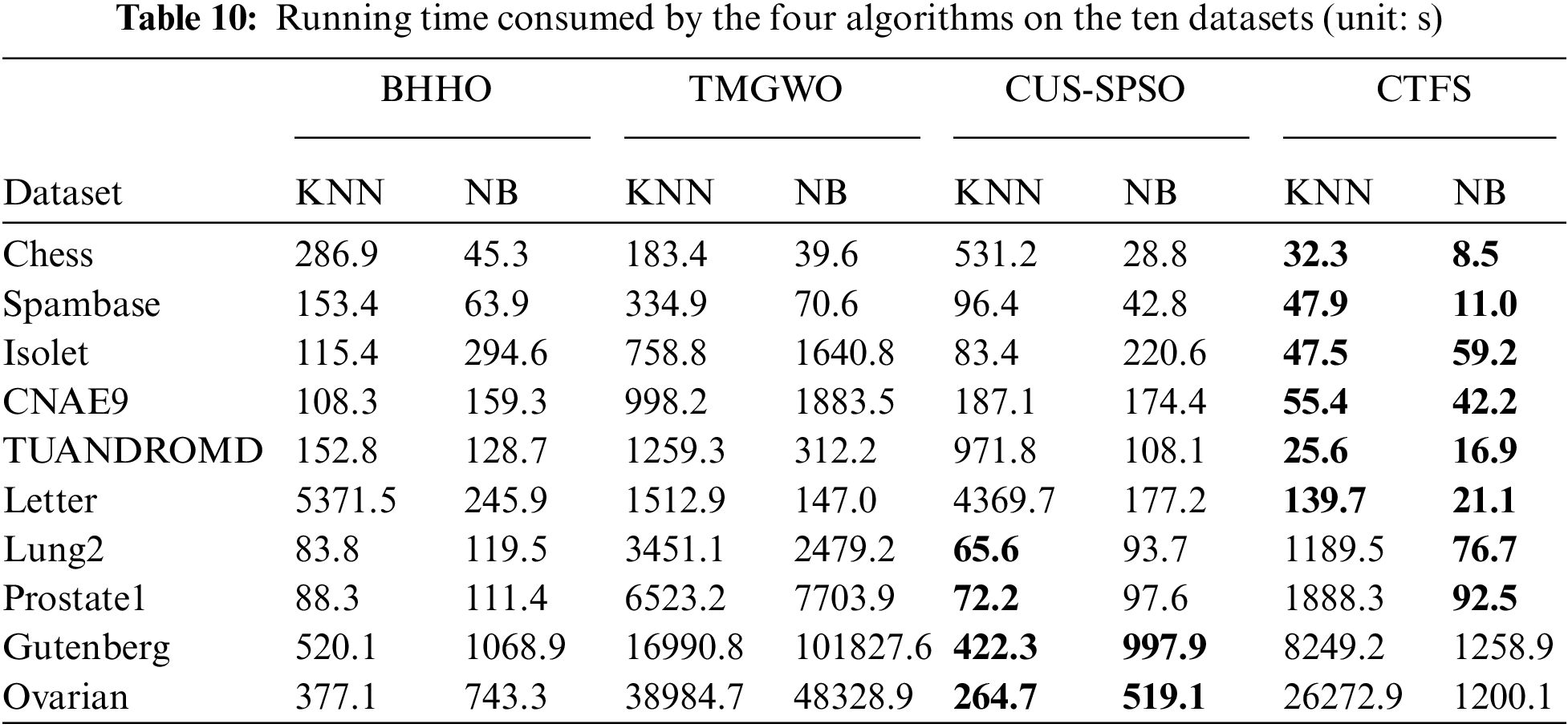
Fig. 5 intuitively displays the running time of algorithms on ten datasets when using KNN and Bayesian as classifiers. The length of the orange rectangle represents the proportional running time of the CTFS algorithm. Because of the long running time of the TMGWO algorithm on high-dimensional datasets, we convert the running time by using the proportional running time of a single algorithm in the total running time of all algorithms as the value of the length. The algorithm proposed in this paper has a shorter length on most datasets, especially using Bayesian as a classifier; that is, the running time is relatively short.

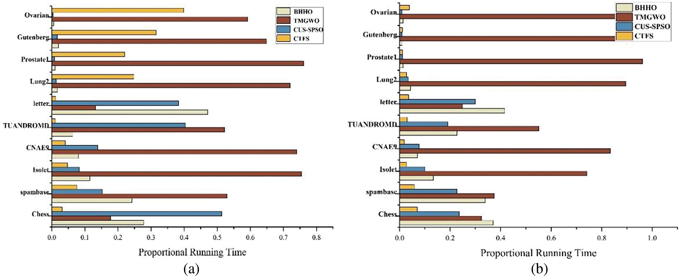
Figure 5: Proportional running time of different algorithms on ten datasets (a) KNN classifier (b) Bayesian classifier

6  Conclusions

This paper introduces a novel wrapper feature selection algorithm called CTFS. Initially, the modified sparse autoencoder network is integrated with mutual information to achieve dominance over each feature. Following that, the informative attributes can be located in the optimal feature subset by a designed contribution tracking strategy, which performs in a dominance accumulation form. The computational results on multiple test datasets illustrate that the CTFS algorithm outperforms advanced algorithms in terms of classification accuracy, recall rate, F1 score, and dimension reduction capability. However, compared to other algorithms, the experimental results of runtime for high-dimensional datasets are not significantly superior. Subsequent research endeavors will focus on further reducing the training time in addressing ultra-high-dimensional feature selection problems.

Acknowledgement: The authors would like to express their gratitude to the editor and the anonymous reviewers for their insightful suggestions, which significantly raised the caliber of this work.

Funding Statement: This work was supported in part by the National Key Research and Development Program of China under Grant (No. 2021YFB3300900); the NSFC Key Supported Project of the Major Research Plan under Grant (No. 92267206); the National Natural Science Foundation of China under Grant (Nos. 72201052, 62032013, 62173076); the Fundamental Research Funds for the Central Universities under Grant (No. N2204017); the Fundamental Research Funds for State Key Laboratory of Synthetical Automation for Process Industries under Grant (No. 2013ZCX11).

Author Contributions: Study conception, design and draft manuscript preparation: Yifan Yu; data collection and editing: Dazhi Wang; analysis and interpretation of results: Yanhua Chen; validation: Hongfeng Wang; project administration and supervision: Min Huang. All authors reviewed the results and approved the final version of the manuscript.

Availability of Data and Materials: The data sets applied in the paper are available in the UCI repository at https://archive.ics.uci.edu/datasets (accessed on 05 April 2024) and the scikit-feature feature selection repository at https://jundongl.github.io/scikit-feature/datasets (accessed on 11 April 2024).

Ethics Approval: Not applicable.

Conflicts of Interest: The authors declare no conflicts of interest to report regarding the present study.

References

1. J. Gui, Z. Sun, S. Ji, D. Tao, and T. Tan, “Feature selection based on structured sparsity: A comprehensive study,” IEEE Trans. Neural Netw. Learn. Syst., vol. 28, no. 7, pp. 1490–1507, 2016. doi: 10.1109/TNNLS.2016.2551724. [Google Scholar] [PubMed] [CrossRef]

2. S. S. Gandhi and S. S. Prabhune, “Overview of feature subset selection algorithm for high dimensional data,” in 2017 Proc. Int. Conf. Inventive Syst. Control (ICISC), Coimbatore, India, 2017, pp. 1–6. [Google Scholar]

3. G. Wang, P. Zhang, D. Wang, H. Chen, and T. Li, “Fast attribute reduction via inconsistent equivalence classes for large-scale data,” Int. J. Approximate Reasoning, vol. 163, 2023, Art. no. 109039. doi: 10.1016/j.ijar.2023.109039. [Google Scholar] [CrossRef]

4. A. A. Alhussan and S. K. Towfek, “5G resource allocation using feature selection and greylag goose optimization algorithm,” Comput. Mater. Contin., vol. 80, no. 1, pp. 1180–1181, 2024. doi: 10.32604/cmc.2024.049874. [Google Scholar] [CrossRef]

5. Z. Zeng, A. Tang, S. Yi, X. Yuan, and Y. Zhu, “A heuristic radiomics feature selection method based on frequency iteration and multi-supervised training mode,” Comput. Mater. Contin., vol. 79, no. 2, pp. 2278–2279, 2024. doi: 10.32604/cmc.2024.047989. [Google Scholar] [CrossRef]

6. M. Braik, A. Hammouri, H. Alzoubi, and A. Sheta, “Feature selection based nature inspired capuchin search algorithm for solving classification problems,” Expert Syst. Appl., vol. 235, 2024, Art. no. 121128. doi: 10.1016/j.eswa.2023.121128. [Google Scholar] [CrossRef]

7. H. Zhang, J. Wang, Z. Sun, J. M. Zurada, and N. R. Pal, “Feature selection for neural networks using group lasso regularization,” IEEE Trans. Knowl. Data Eng., vol. 32, no. 4, pp. 659–673, 2019. doi: 10.1109/TKDE.2019.2893266. [Google Scholar] [CrossRef]

8. J. Yu, “Manifold regularized stacked denoising autoencoders with feature selection,” Neurocomputing, vol. 358, pp. 235–245, 2019. doi: 10.1016/j.neucom.2019.05.050. [Google Scholar] [CrossRef]

9. R. J. Urbanowicz, M. Meeker, W. La Cava, R. S. Olson, and J. H. Moore, “Relief-based feature selection: Introduction and review,” J. Biomed. Inform., vol. 85, pp. 189–203, 2018. doi: 10.1016/j.jbi.2018.07.014. [Google Scholar] [PubMed] [CrossRef]

10. H. Peng, F. Long, and C. Ding, “Feature selection based on mutual information criteria of max-dependency, max-relevance, and min-redundancy,” IEEE Trans. Pattern Anal. Mach. Intell., vol. 27, no. 8, pp. 1226–1238, 2005. doi: 10.1109/TPAMI.2005.159. [Google Scholar] [PubMed] [CrossRef]

11. G. Roffo, S. Melzi, U. Castellani, A. Vinciarelli, and M. Cristani, “Infinite feature selection: A graph-based feature filtering approach,” IEEE Trans. Pattern Anal. Mach. Intell., vol. 43, no. 12, pp. 4396–4410, 2020. doi: 10.1109/TPAMI.2020.3002843. [Google Scholar] [PubMed] [CrossRef]

12. E. Hancer, B. Xue, and M. Zhang, “Differential evolution for filter feature selection based on information theory and feature ranking,” Knowl.-Based Syst., vol. 140, no. 10, pp. 103–119, 2018. doi: 10.1016/j.knosys.2017.10.028. [Google Scholar] [CrossRef]

13. K. Yan and D. Zhang, “Feature selection and analysis on correlated gas sensor data with recursive feature elimination,” Sens. Actuators B: Chem., vol. 212, pp. 353–363, 2015. doi: 10.1016/j.snb.2015.02.025. [Google Scholar] [CrossRef]

14. W. Liu and J. Wang, “Recursive elimination-election algorithms for wrapper feature selection,” Appl. Soft Comput., vol. 113, 2021, Art. no. 107956. doi: 10.1016/j.asoc.2021.107956. [Google Scholar] [CrossRef]

15. M. B. Kursa and W. R. Rudnicki, “Feature selection with the Boruta package,” J. Stat. Softw., vol. 36, no. 11, pp. 1–13, 2010. doi: 10.18637/jss.v036.i11. [Google Scholar] [CrossRef]

16. A. K. Naik and V. Kuppili, “An embedded feature selection method based on generalized classifier neural network for cancer classification,” Comput. Biol. Med., vol. 168, 2024, Art. no. 107677. doi: 10.1016/j.compbiomed.2023.107677. [Google Scholar] [PubMed] [CrossRef]

17. A. Jiménez-Cordero, J. M. Morales, and S. Pineda, “A novel embedded min-max approach for feature selection in nonlinear support vector machine classification,” Eur. J. Oper. Res., vol. 293, no. 1, pp. 24–35, 2021. doi: 10.1016/j.ejor.2020.12.009. [Google Scholar] [CrossRef]

18. M. Braik, “Enhanced Ali Baba and the forty thieves algorithm for feature selection,” Neural Comput. Appl., vol. 35, no. 8, pp. 6153–6184, 2023. doi: 10.1007/s00521-022-08015-5. [Google Scholar] [PubMed] [CrossRef]

19. X. Song, Y. Zhang, Y. Guo, X. Sun, and Y. Wang, “Variable-size cooperative coevolutionary particle swarm optimization for feature selection on high-dimensional data,” IEEE Trans. Evol. Comput., vol. 24, no. 5, pp. 882–895, 2020. doi: 10.1109/TEVC.2020.2968743. [Google Scholar] [CrossRef]

20. L. Qu, W. He, J. Li, H. Zhang, C. Yang and B. Xie, “Explicit and size-adaptive PSO-based feature selection for classification,” Swarm Evol. Comput., vol. 77, 2023, Art. no. 101249. doi: 10.1016/j.swevo.2023.101249. [Google Scholar] [CrossRef]

21. H. Pan, S. Chen, and H. Xiong, “A high-dimensional feature selection method based on modified gray wolf optimization,” Appl. Soft Comput., vol. 135, 2023, Art. no. 110031. doi: 10.1016/j.asoc.2023.110031. [Google Scholar] [CrossRef]

22. F. G. Mohammadi and M. S. Abadeh, “Image steganalysis using a bee colony based feature selection algorithm,” Eng. Appl. Artif. Intell., vol. 31, pp. 35–43, 2014. doi: 10.1016/j.engappai.2013.09.016. [Google Scholar] [CrossRef]

23. K. Chen, B. Xue, M. Zhang, and F. Zhou, “Correlation-guided updating strategy for feature selection in classification with surrogate-assisted particle swarm optimization,” IEEE Trans. Evol. Comput., vol. 26, no. 5, pp. 1015–1029, 2021. doi: 10.1109/TEVC.2021.3134804. [Google Scholar] [CrossRef]

24. X. Wang, H. Shangguan, F. Huang, S. Wu, and W. Jia, “MEL: Efficient multi-task evolutionary learning for high-dimensional feature selection,” IEEE Trans. Knowl. Data Eng., vol. 36, no. 8, pp. 4020–4033, 2024. doi: 10.1109/TKDE.2024.3366333. [Google Scholar] [CrossRef]

25. K. Chen, B. Xue, M. Zhang, and F. Zhou, “An evolutionary multitasking-based feature selection method for high-dimensional classification,” IEEE Trans. Cybern., vol. 52, no. 7, pp. 7172–7186, 2022. doi: 10.1109/TCYB.2020.3042243. [Google Scholar] [PubMed] [CrossRef]

26. L. Peng, Z. Cai, A. A. Heidari, L. Zhang, and H. Chen, “Hierarchical Harris hawks optimizer for feature selection,” J. Adv. Res., vol. 53, pp. 261–278, 2023. doi: 10.1016/j.jare.2023.01.014. [Google Scholar] [PubMed] [CrossRef]

27. I. Lahmar, A. Zaier, M. Yahia, and R. Boaullegue, “A novel improved binary harris hawks optimization for high dimensionality feature selection,” Pattern Recognit. Lett., vol. 171, no. 6, pp. 170–176, 2023. doi: 10.1016/j.patrec.2023.05.007. [Google Scholar] [CrossRef]

28. M. Abdel-Basset, D. El-Shahat, I. El-Henawy, V. H. C. De Albuquerque, and S. Mirjalili, “A new fusion of grey wolf optimizer algorithm with a two-phase mutation for feature selection,” Expert Syst. Appl., vol. 139, no. 3, pp. 432, 2020. doi: 10.1016/j.eswa.2019.112824. [Google Scholar] [CrossRef]

29. J. Zhou and Z. Hua, “A correlation guided genetic algorithm and its application to feature selection,” Appl. Soft Comput., vol. 123, 2022, Art. no. 108964. doi: 10.1016/j.asoc.2022.108964. [Google Scholar] [CrossRef]

30. S. Han, J. Pool, J. Tran, and W. Dally, “Learning both weights and connections for efficient neural networks,” in 2015 Adv. Neural Inf. Proces. Syst. (NIPS), Montreal, QC, Canada, 2015, pp. 1135–1143. [Google Scholar]

31. D. C. Mocanu, E. Mocanu, P. Stone, P. H. Nguyen, M. Gibescu and A. Liotta, “Scalable training of artificial neural networks with adaptive sparse connectivity inspired by network science,” Nat. Commun., vol. 9, no. 1, 2018, Art. no. 2383. doi: 10.1038/s41467-018-04316-3. [Google Scholar] [PubMed] [CrossRef]

32. Z. Atashgahi et al., “Quick and robust feature selection: The strength of energy-efficient sparse training for autoencoders,” Mach. Learn., vol. 111, no. 1, pp. 377–414, 2021. doi: 10.1007/s10994-021-06063-x. [Google Scholar] [CrossRef]

33. G. Sokar, Z. Atashgahi, M. Pechenizkiy, and D. C. Mocanu, “Where to pay attention in sparse training for feature selection?” in 2022 Adv. Neural Inf. Process. Syst (NIPS), New Orleans, LA, USA, 2022, pp. 1627–1642. [Google Scholar]

34. J. Li et al., “Feature selection: A data perspective,” ACM Comput. Surv., vol. 50, no. 6, pp. 1–45, 2017. doi: 10.1145/3136625. [Google Scholar] [CrossRef]