A Study on Polyp Dataset Expansion Algorithm Based on Improved Pix2Pix

1  Introduction

Colorectal cancer (CRC) is one of the most prevalent cancers in clinical settings, with notably high incidence and mortality rates. According to the latest global cancer burden data released in 2020 by the International Agency for Research on Cancer of the World Health Organization, CRC has risen to the third most common cancer globally, with 1.93 million new cases, accounting for 10.6% of all new cancer diagnoses. Among the leading causes of cancer-related death worldwide, CRC now ranks second, with 930,000 deaths. Additionally, most patients are diagnosed at an intermediate or advanced stage, where the survival rate drops significantly to just 10%. However, if CRC is detected early, treatment can increase the survival rate to over 90% [1].

Thus, early colorectal endoscopy and timely resection are crucial. Traditionally, examinations have relied on direct clinical observation, a method that is both subjective and prone to physician fatigue and variable experience levels. To address these limitations, a research team led by the Mayo Clinic conducted a study on how artificial intelligence (AI) impacts the rate of missed colorectal carcinoma cases [2]. Their findings showed a polyp leakage rate of 25% in routine procedures, which dropped to 15.5% in patients undergoing their first AI-assisted colonoscopy. Despite these advances, there are still challenges in current algorithms. Most polyp detection methods enhance detection and segmentation by applying preprocessing and post-processing on existing datasets. However, polyp detection remains challenging due to the high variability in polyp shape and color, as well as the limited availability of existing datasets. Creating a robust dataset requires extensive manual annotation by professionals, representing a considerable workload. Therefore, in response to these issues, scholars have proposed many solutions for data augmentation. These solutions are mainly distributed in the fields of image denoising and dataset augmentation. The MedDeblur [3] and DarkDeblur [4] proposed by Sharif et al. are typical representatives of image denoising. The data augmentation scheme we adopt is to expand the dataset through graph generation.

Since the generative adversarial network (GAN) was proposed by Goodfellow et al. [5] in 2014, it has attracted wide attention. GAN is a generative model composed of a generator and a discriminator that generates realistic data through adversarial training. The training mode of the generator and discriminator game with each other is brilliant in the field of computer vision. At the same time, due to the particularity of medical data sets, various medical data set expansion schemes based on GAN emerge endlessly. In 2017, Calimeri et al. [6] used the Gan network to expand Magnetic Resonance Imaging (MRI) image data of large brain, effectively improving the generalization ability of the diagnostic algorithm. Recently, to expand the polyp data set, GAN based processing scheme has also begun to appear. Golhar et al. [7] expanded the polyp dataset by using Gan to migrate the style of polyp images. Although different types of polyp images can be obtained through this expansion scheme, it is difficult to obtain polyp images with more abundant feature information. De Almeida Thomaz et al. [8] first used GAN to generate a polyp mask, and then placed the polyp mask on the polyp-free part. It used two different frames throughout the process. Although this method can obtain new polyp images with different shapes, the process is cumbersome and the image resolution is not high. Shin et al. [9] used the method of edge extraction and inputted the extracted edge image into conditional generative adversarial networks (cGAN) to obtain a new polyp image. cGAN is a generative model that introduces conditional control based on GAN, enabling the generated data to meet specific attributes. Although this method can generate realistic polyp images, the process of performing edge extraction for each set of images is cumbersome, and the generated polyp features are relatively weak. In contrast, our proposed polyp generation approach simply overlays a mask on the target area and infers the polyp sample, making the process significantly more efficient. Additionally, by placing the mask in random positions, we enhance the feature richness of the generated samples. Qadir et al. [10] used the existing image mask to input the conditional Gans to obtain a new polyp image. While flexible, this method generates limited polyp features and is prone to reflection interference. To address the issue of limited information in generated samples, we employ a random overlay of masks. Additionally, the attention mechanism used in our approach helps mitigate reflection interference. The current research faces several challenges, including a cumbersome process, insufficient information in generated polyp samples, and susceptibility to interference from reflections.

In this study, we completed the selection and improvement of the confrontation generation model according to the research goal of efficiently generating high-quality polyp samples to expand our polyp data set. The main contributions of this work are as follows:

1.    After several comparison tests in the generator, we added the attention mechanism at the optimal position. It helps us to eliminate the interference caused by the reflection of foreign objects in the image during the image generation process.

2.    We examined how various loss strategies affect the stability of creating adversarial models and select the best loss strategy.

3.    We enriched the information of generated polyp samples by randomly splicing different angle masks. Moreover, we validate the method in the experimental section.

The remaining parts of the paper are organized as follows. Section 2 presents the framework for polyp generation and the preparation scheme for the input images. In Section 3, We experiment and analyze the proposed scheme to verify its effectiveness. Concluding remarks are given in Section 4.

2  Methods

Image generation tasks based on deep learning are often completed on GAN or cGAN. GAN consists of two networks: a generator and a discriminator. The generator learns to generate realistic data, while the discriminator strives to distinguish between real data and generated data. The two generate data that is closest to reality through competition and confrontation, but the content generated through GAN is often uncontrollable. cGAN introduces conditional information for constraints based on GAN, improving the controllability and flexibility of data. Therefore, in order to complete the task of dataset expansion, many experts and scholars often use cGAN for dataset expansion. However, using cGAN to complete the polyp dataset expansion task will result in overly single shapes, making it difficult to improve the detection performance of subsequent models. Pix2Pix [11] is an image-to-image translation model based on cGAN. Pix2Pix achieves the required output by using real image inputs rather than noise vectors. More information gives the generator the ability to produce more tailored outcomes. To meet our task requirements, we employ an improved Pix2Pix network model. Fig. 1 shows the specific process and architecture of the network model for polyp generation. We first place the mask at random positions outside the polyp and pair it with the real image to obtain the weight for polyp removal. Then, we place the mask on the polyp and pair it with real polyp images to generate a model for obtaining the weights of polyp generation. For these two transformations, we use the same generation model. We can infer an image without polyps by using the first weight. Meanwhile, we will get a newly generated image with polyps by using the second weight.

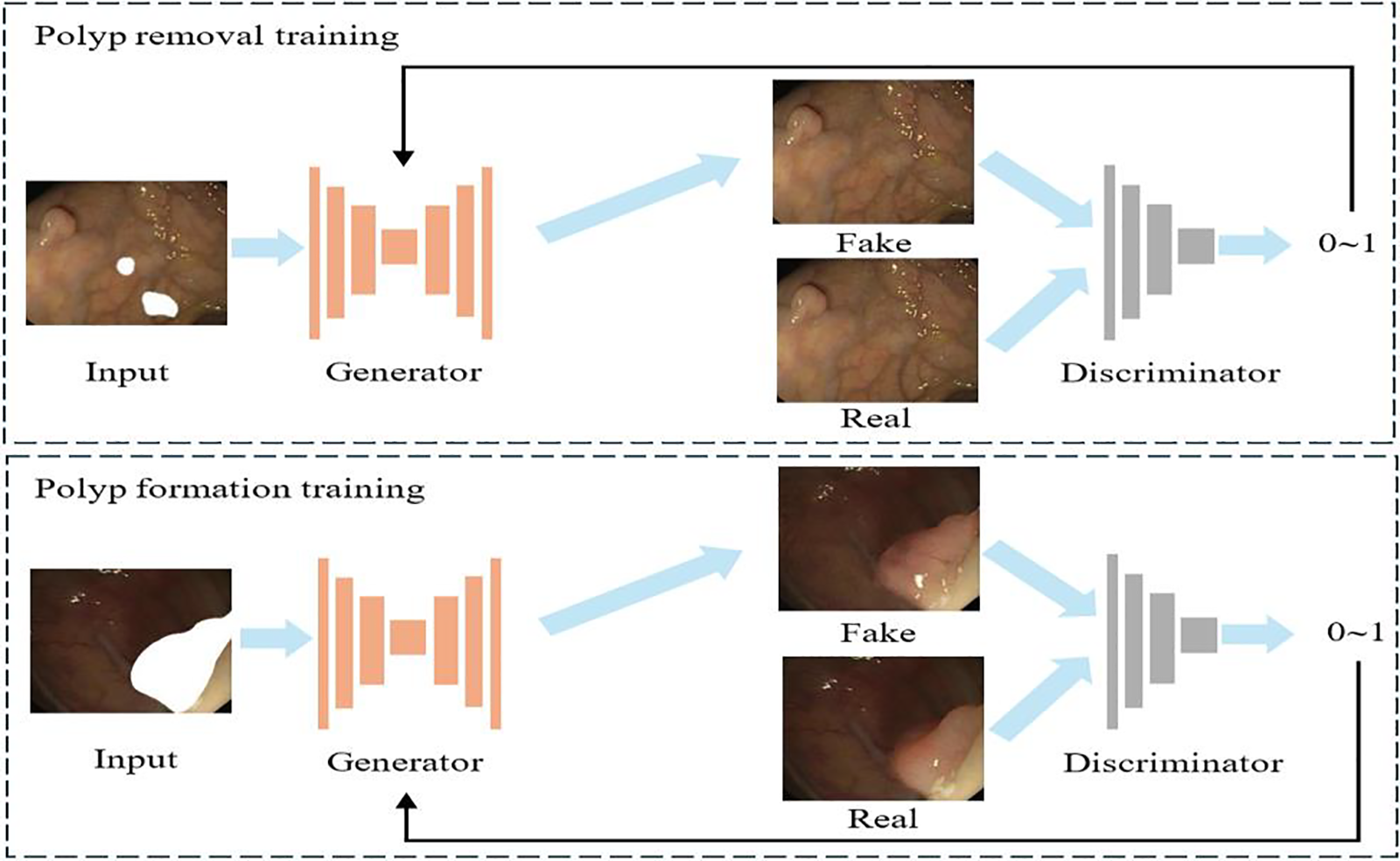
Figure 1: Polyp generation scheme

2.1 Model Structure

The algorithm we proposed is polyp generation algorithm based on attention and multi-shape mask (PGAM), with its generator and discriminator architectures shown in Fig. 2. We chose U-Net as its generator. The reason for this is the close fit between the U-Net network architecture and the specific needs of our tasks. U-Net uses a layer-by-layer sampling approach. This effectively captures features such as polyp edge textures and helps generate realistic, detailed polyp images. Additionally, its skip connections pass low-level features from the encoder directly to the corresponding decoder layers. This reduces information loss. As a result, the network can capture fine details effectively, even on small datasets like the polyp dataset, thereby enhancing image quality. Therefore, combining these properties and the requirements of our tasks, we chose U-Net as our generator. As a discriminator, PatchGAN divides images into small patches for separate discrimination. This approach effectively captures fine textures and structural details in polyp images, ensuring that generated images are consistent with real images in terms of detail. Additionally, the small sample size of the polyp dataset increases the risk of overfitting. Focusing on local regions, PatchGAN reduces this risk. Moreover, this approach requires fewer computational resources compared to other methods, meeting our needs.

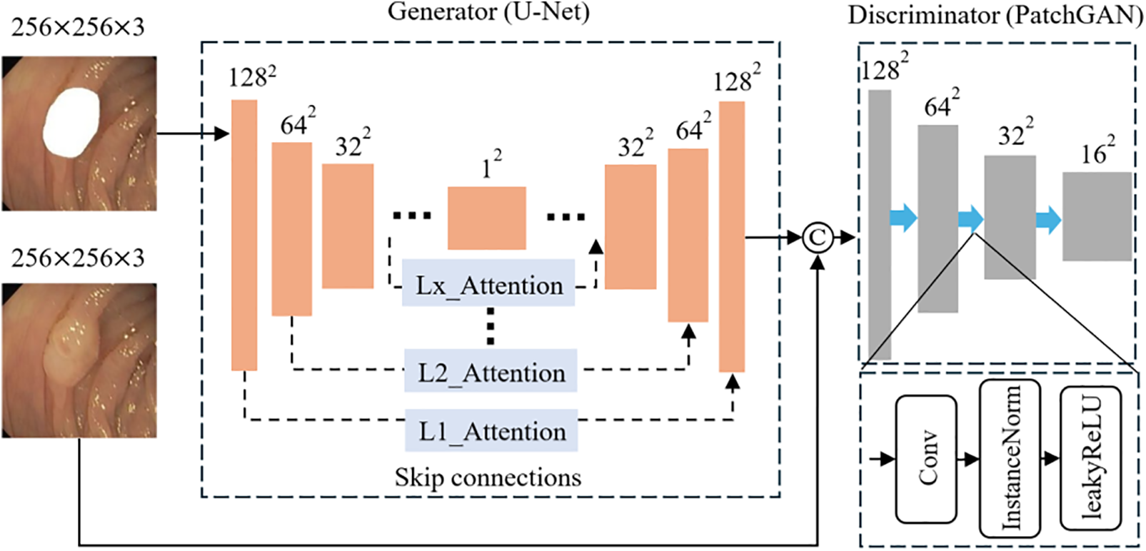
Figure 2: Polyp generation algorithm based on attention and multi-shape mask (PGAM)

On the other hand, we modified the generator to filter out the generation interference brought on by different negative effects in the polyp images. Simultaneously, we adopted Wasserstein GAN with Gradient Penalty (WGAN-GP) [12] as the loss function of the model. Secondly, we merged various masks to generate polyps with different shapes. It helps us address the issue of stagnating model identification performance.

As shown in Fig. 2, we feed a pair of 256 × 256 × 3 paired images into the model. The image with the mask enters the generator to generate polyps. In the generator, we obtain the down-sampled feature map 16 × 16 × 512 by passing through four convolutional layers with a kernel size of 4 × 4 and a stride of 2 in each layer. Then, through four convolutional layers similar to the above, but with no change in the number of channels, we obtain the deepest down-sampled feature map 1 × 1 × 512. The up-sampling process is the opposite. Skip connections concatenate the down-sampled feature maps of each layer with the up-sampled feature maps in the channel dimension. It allows the generated image to retain more details. Meanwhile, for excluding the influence of various disturbances, we add an attention mechanism to the connection part of up-sampling and down-sampling. To explore where the attention mechanism plays the most significant role, we conduct comparative experiments on it, and the results are shown in Section 3.6.

Secondly, we concatenate the fake images generated by the generator with the corresponding real polyp images and input them into the discriminator for discrimination. PatchGAN utilized a combination of Convolution, InstanceNorm and leakyReLU modules to downsample the concatenated images with dimensions of 256 × 256 × 6 to 16 × 16 × 1 patches for discrimination.

2.2 Loss Function

It is commonly recognized that GAN optimizes two models by having the generator and discriminator play a mutual game. In this setup, the loss functions of the discriminator and generator are viewed as part of a minimax game.

The loss function used in our training is shown in Eq. (1). It consists of two parts of losses. LWGP refers to the Generative Adversarial Network loss, and L1 refers to the regularization loss as shown in Eq. (2). G and D refer to the generator and discriminator networks, respectively. λ is used to adjust the balance between losses. The expression argminGmaxD represents the minimax game between the generator and the discriminator. This is the standard approach in GAN training, where the generator tries to minimize the loss while the discriminator tries to maximize it. LWGP solves the problems of gradient vanishing and pattern collapse in traditional GAN training by optimizing Wasserstein distance and introducing gradient penalty terms. Improved the stability of training and the quality of generated samples. The L1 loss function is good at capturing low-frequency information of images. It helps generate smoother and more coherent images. In image generation or restoration tasks, combining WGAN-GP with the L1 loss function can maintain both the diversity and authenticity of generated samples. Meanwhile, it ensures that the generated images are visually clearer and more coherent. This combination strategy fully utilizes the advantages of both, thus achieving good results in practical applications. Therefore, the combination of LWGP and L1 loss functions can help us generate polyp samples stably. LWGP is introduced in Section 2.3. The effectiveness of this combination is validated in Section 3.4.

L=argminG⁡maxDLWGP(G,D)+λL1(G)(1)

L1(G)=Ex,y[∥y−G(x)∥1](2)

2.3 WGAN-GP

Training instability is a common problem in GAN. Therefore, we seek a stable loss strategy suitable for polyp generation tasks. Currently, Wasserstein GAN (WGAN) [13] and WGAN-GP are widely applied to improve generative model stability. The WGAN formula, shown in Eq. (3), includes Pg, the generator’s distribution, and Pr, the real data distribution. This function works by maximizing the score of real samples and minimizing the score of generated samples. This enables the discriminator to effectively distinguish real from generated samples. WGAN approximates the real image distribution more accurately using Wasserstein distance. This significantly enhances the quality and diversity of generated polyp images. However, it relies on weight clipping to meet the Lipschitz continuity constraint. Weight clipping can limit discriminator performance, as it often causes gradient vanishing or exploding. This, in turn, affects the model’s learning efficiency. The formula for WGAN-GP is shown in Eq. (4). It combines the Wasserstein distance with a gradient penalty, significantly improving training stability. This ensures that generated polyp images are coherent and free from distortion. WGAN-GP also reduces the risk of overfitting on small sample datasets, preventing generated polyp samples from being overly repetitive and enhancing generalization. The gradient penalty ensures the discriminator’s gradient approaches 1 at interpolated samples, further improving sample quality and reducing the risk of mode collapse. This strengthens gradient flow, allowing the model to capture complex edges and texture details in polyp images.

LW=Ex~∼Pg[D(x~)]−Ex∼Pr[D(x)]⏟Originalcriticloss(3)

LWGP=Ex~∼Pg[D(x~)]−Ex∼Pr[D(x)]⏟Original critic loss +λEx^∼Px^[(∥∇x^D(x^)∥2−1)2]⏟gradient penalty (4)

2.4 Attention Mechanism

In image generation, reflections in the picture have adverse effects on the removal and generation of polyps. For this problem, we introduce the attention mechanism in the generator. Since polyps have distinct shape and positional features, location information is crucial. Coordinated attention (CA) enhances spatial awareness through coordinate encoding, helping the network more accurately capture polyp edges and fine structures. Additionally, CA dynamically assigns weights to different channels, allowing the network to focus on important areas in the feature map. For polyp images with high diversity and rich detail, CA enables the model to identify and generate valuable features more precisely, enhancing generation quality. This superiority is demonstrated in our experiments. Furthermore, CA is lighter and more efficient than other attention mechanisms, aligning with our need for efficient generation. Therefore, we selected CA as our attention mechanism.

CA is an efficient attention mechanism. By embedding location information into channel attention, the network can focus on a larger area without introducing significant computational overhead. Its structure is shown in Fig. 3, and the effectiveness of this module will be verified in Section 3.7.

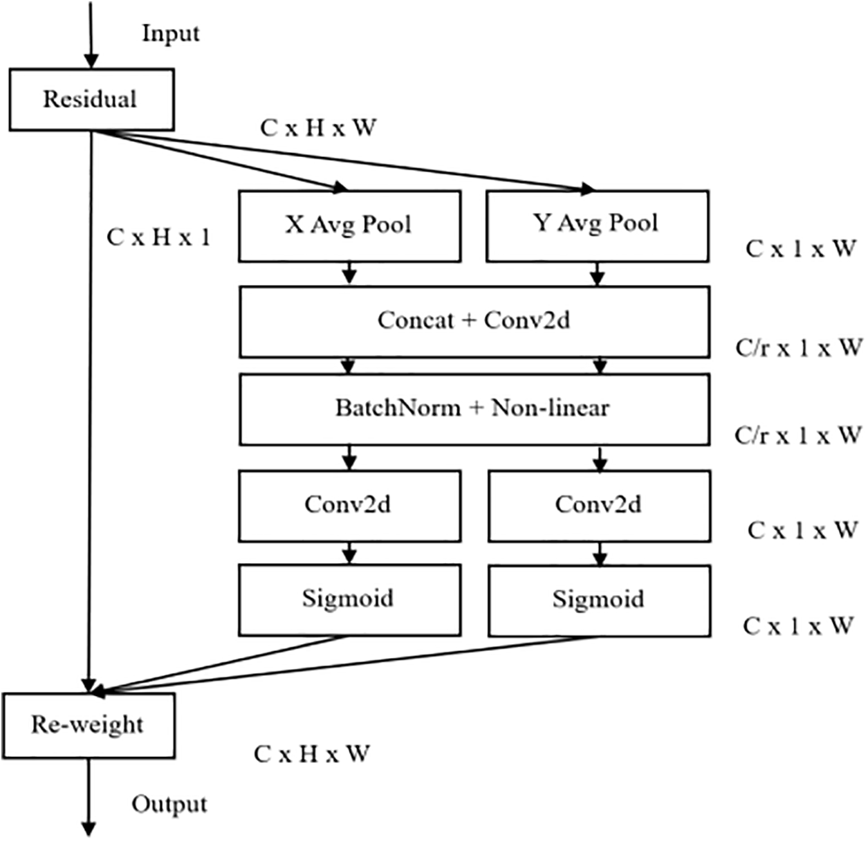
Figure 3: CA attention structure

2.5 Process of Training

The model takes input in the form of mask overlays and paired real images. The generator produces realistic images, while the discriminator’s task is to distinguish between real and fake images generated by the generator. During training, the generator and discriminator alternate in updating their parameters. The generator aims to deceive the discriminator into classifying the generated images as real, while the discriminator continuously improves its ability to distinguish between real and fake images. This adversarial training approach drives the generator to gradually learn how to generate high-quality images. Meanwhile, the discriminator becomes increasingly accurate. After multiple iterations, the model reaches a state of convergence, allowing us to obtain the final weights of the Pix2Pix model.

In this training, we aim to obtain the weights for removing polyps and the weights for generating polyps. This is so that we can generate polyp samples in the inference phase. Through passing the mask-covered image and the original image into the adversarial model, the model is able to generate in the masked region based on the matrix information of the original image. After continuous confrontation, a target image similar to the original image is generated and we get the corresponding training weights. The purpose of the mask is to provide information about the edge and position of the polyp, and to inform the model about the shape and area of the polyp to be generated or removed. In the subsequent inference phase, we just need to place the mask at the appropriate location. Then, using the training process to get the corresponding weights can realize the removal and generation of polyps in the mask area.

2.5.1 Polyp-Free Image Generation

The polyp generation scheme we adopt is to first remove the existing polyp, and then generate new polyp at random positions to achieve the goal of expanding the polyp dataset.

In this work, we take the existing polyp mask and extract it. Then, we set restriction regions in the polyp part of the polyp image by Open Source Computer Vision Library (OpenCV). Finally, we superimposed the mask to the region outside the restriction. The image obtained is shown in Fig. 4. Through training with both the original image and the mask overlay, we can obtain efficient weights capable of removing polyps. This weight allows us to produce photos devoid of polyps. The first training cycle is depicted in Fig. 5, Input 1 is an image of the original polyp image with a mask added. Input 2 is a produced image of the mask area being repaired during training. Output is the original polyp image without a mask. Fig. 5. shows that we are able to produce very comparable images to the original in the mask region using our generative model.

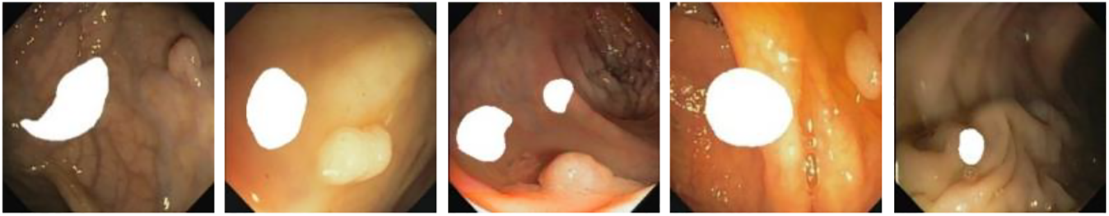
Figure 4: Masks setting for polyp removal training

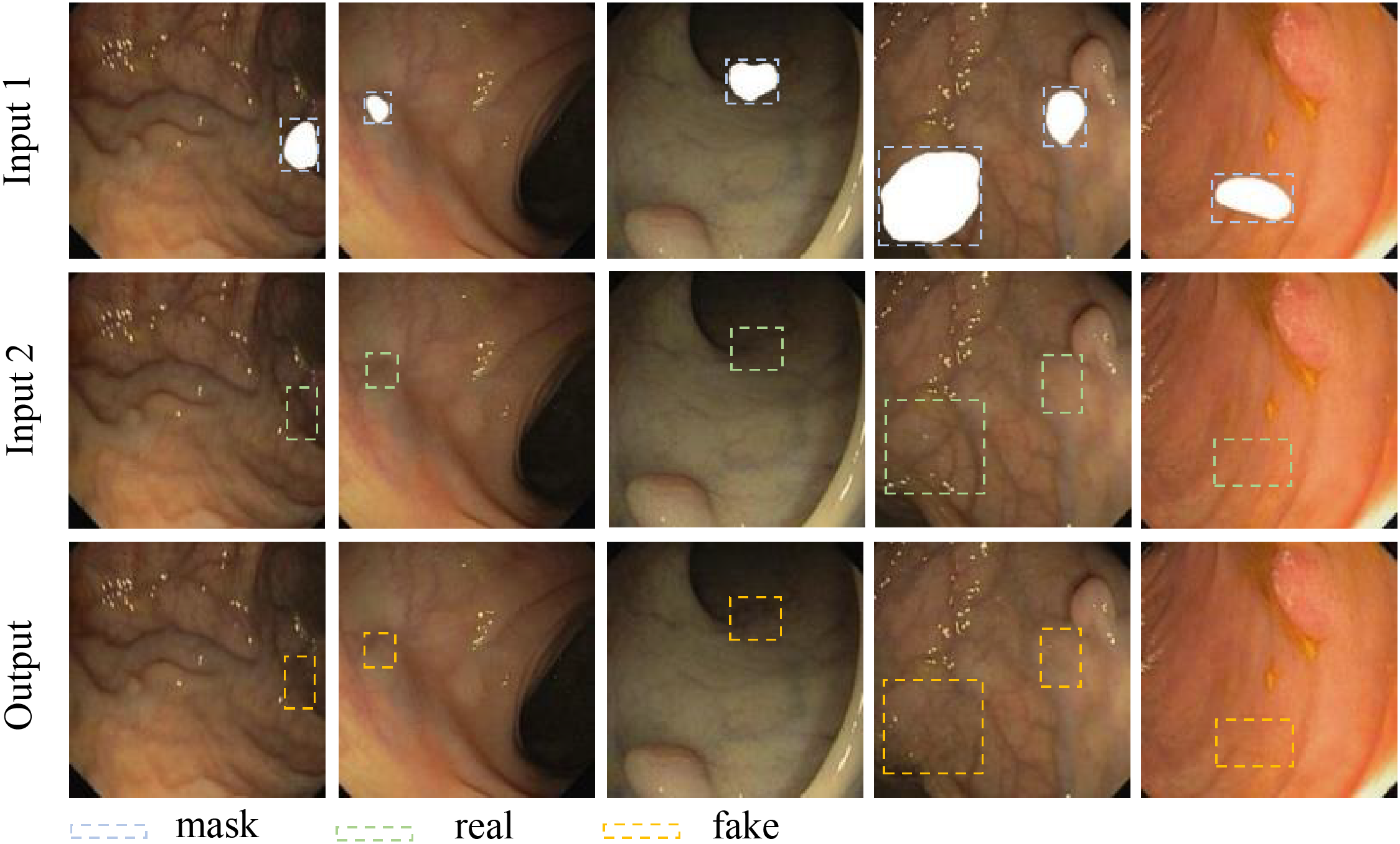
Figure 5: Training of polyp elimination

Upon completion of the first round of training, the resulting weights are applied for inference on images with polyp masks. Consequently, this leads to the generation of polyp-free images. If only the original mask is applied to the polyp for inference, the resulting polyp removal image will have visible polyp boundaries around the disappeared polyp as shown in Fig. 6a. Toward a more perfect polyp-free image, we utilize OpenCV to expand the mask boundary to cover the shaded portion as shown in Fig. 6b. Its inference produces an even more perfect image. In Fig. 6, (a) has a more pronounced sense of boundary than (b), which is not conducive to further polyp formation.

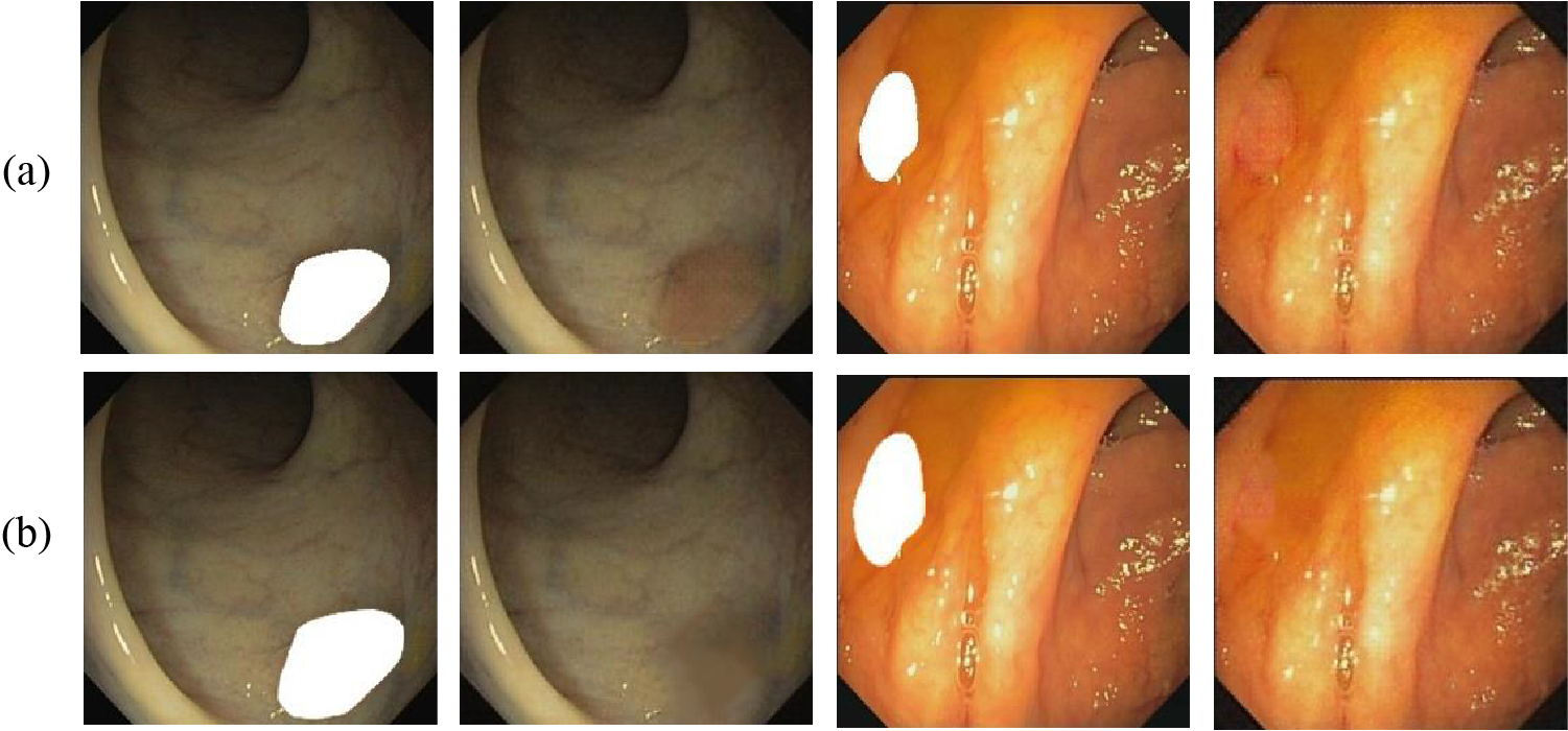
Figure 6: Masks designed for removing shadow interference (a) original mask (b) expand mask boundary

To obtain new polyp images that are more balanced, we will select polyp images from each site and input them into the model for inference to obtain polyp-free images, which will be shown in Section 3.

2.5.2 Polyp Image Generation

Following the generation of pictures devoid of polyps, various shaped polyps are produced on the freshly created images. In this work, we employ the same generation model as before. Our masks were set up in such a way that the polyps were directly superimposed with the paired masks as shown in Fig. 7. After that we need to pair the image containing the polyp mask with the image without the mask and pass it into the network for training. Consequently, the training weights for polyp formation were obtained. As can be seen in Fig. 8, Input 1 and Input 2 are the input-paired images, while Output is the generated image that generates polyps in the blank area of the image during training. It is also input into the model together for training, so as to obtain the weights that can generate polyps. From the output images, it can be seen that the polyp pattern generated by the generative network is highly similar to the original images.

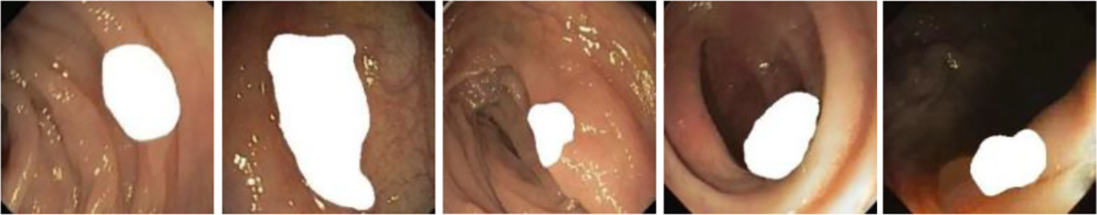
Figure 7: Masks setting for polyp generation training

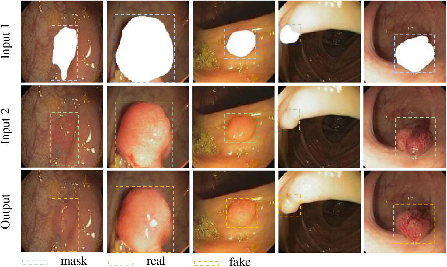
Figure 8: Training of polyp formation

Simultaneously, inspired by the literature [10]. For increasing the diversity of the generated images as well as improve the performance of the subsequent detection and segmentation models, we consider combining two or more different polyp masks randomly and placing them in different scenes to generate polyp images with different shapes as shown in Fig. 9. This approach aims to increase the diversity of the generated images and improve the performance of subsequent detection and segmentation models. The effectiveness of the method will be demonstrated in Section 3.9.

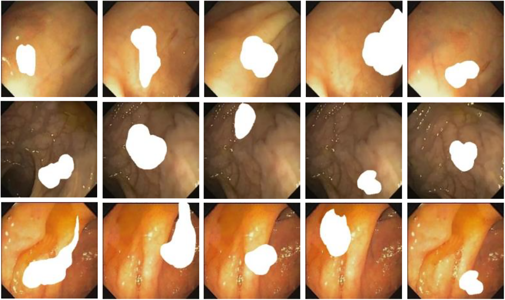
Figure 9: Endoscope images using randomly generated masks

2.6 Models Used to Evaluate Data Sets

To quantitatively evaluate our combined dataset, we selected mainstream models for polyp detection and segmentation. It allows us to compare different generation scenarios.

For the target detection of polyps, we mainly choose three mainstream target detection models, which are Faster R-CNN ResNet101 (Faster Region-based Convolutional Neural Network with Residual Networks 101 layers) [14], Faster R-CNN Inception Resnet v2, and R-FCN ResNet101 (Region-based Fully Convolutional Network with Residual Networks 101 layers) [15]. Faster R-CNN extracts the corresponding feature maps by inputting the images into the network. Simultaneously, it uses the RPN (Region Proposal Network) to generate candidate frames and projects them onto the feature map to obtain the corresponding feature matrices. Finally, each feature matrix is scaled to a 7 × 7 sized feature map by ROI (Region of interest) pooling layer and then the prediction is obtained by spreading the fully connected layers.

The R-FCN neural network is fully convolutional. As the number of network layers increases, not only does the detection accuracy improve, but the speed is also significantly enhanced due to shared parameters.

Meanwhile, we used three mainstream segmentation models to evaluate the role of synthetic polyps. They are TernausNet-16 [16], AlbuNet-34 and MDeNetplus [17]. All three segmentation models are based on the mainstream segmentation framework U-Net. The U-Net algorithm performs exceptionally well in the field of medical image segmentation. It is particularly suited for tasks with small sample sizes, unbalanced data, and a strong need to preserve detailed information. It has been widely used in tumor segmentation, organ segmentation, cell segmentation, etc. and has become one of the important algorithms in the field of image segmentation. TernausNet-16 model uses VGG-16 (Visual Geometry Group-16 Layers) as the encoder network, while AlbuNet-34 uses ResNet-34 as the encoder and improves the jump-connectivity method of U-Net. MDeNetplus not only has jump connections from the encoder layer to the decoder layer but also has feedback connections. The feedback connection sums the activation maps of similar layers from different decoders.

3  Experiment and Analysis

3.1 Experimental Conditions

The training is conducted on a computer running 64-bit Windows 10 system, CUDA 10.1, CUDNN 7.6, NVIDIA GeForce RTX 3060 graphics card, Intel(R) Core (TM) i7-10700K CPU; the software environment for algorithmic experiments adopts Python 3.7 and PyTorch 2.2.1.

For model training, the batch size was set to 2 and the number of training epochs was preset to 200. In the training, the Adam optimizer is used, the initial learning rate is 0.0002, and the norm is chosen as an instance. During the training process, we first removed the black borders from the images in the dataset. Next, we uniformly resized the images to 256 × 256 pixels, with the spliced images being 512 × 256 pixels. To augment the dataset, we applied random geometric transformations such as scaling, rotation, translation, and blocking. Through changing the image size, the dataset is enhanced with random geometry. Random geometric enhancement and random light enhancement are performed on the dataset by changing the saturation and brightness of the image. During the training process, we mainly focus on the convergence trend of the generator and discriminator losses. Ideally, the generator and discriminator losses will reach a balance. In experiments, we sometimes observe that the losses remain unchanged for a long time or fluctuate significantly. In such cases, we adjust the learning rate to 0.0001 to stabilize the training process. Additionally, we may change the loss strategy or reduce the batch size to make the training more stable.

3.2 Dataset

In training and evaluating the performance, we mainly use three common datasets. They are CVC-ClinicDB dataset [18], CVC-Clinic VideoDB dataset [19] and ETIS-LARIB dataset [20]. Among them, the CVC-ClinicDB dataset is used to generate the training of the model, which is also used to combine to generate a new polyp dataset. CVC-Clinic VideoDB and ETIS-LARIB datasets are used for the testing part in the comparison of the target detection and segmentation performance, respectively.

CVC-ClinicDB is an open-access dataset of 612 images with a resolution of 384 × 288 from 31 colonoscopy sequences. It is used for medical image segmentation. CVC-Clinic VideoDB contains 18 SD (384 × 288 pixels) videos. In this dataset, a total of 10,025 frames out of 11,954 frames contain a polyp. For the evaluation of detection models, we use the whole 11,954 frames as a test set.

The ETIS-LARIB dataset contains 196 still images extracted from 34 colonoscopy videos. The image has an HD (high definition) resolution of 1255 × 966 pixels. In this dataset, 44 different polyps were presented in 196 images. Experienced clinicians annotate the polyp segmentation mask on each image.

3.3 Process of Reasoning

In the inference process, our goal is to reason about the weights obtained in the training phase. We proceed in two steps. First, we used the weights to reason about polyp removal. Then, we obtain images without polyps. They provide the background for our polyp generation inference. The second step is to perform polyp generation on the obtained background images. At this point, we will have a new sample.

3.3.1 Polyp Elimination Reasoning

For this task, our goal is to utilize the weights obtained from the first round of training to remove polyps. We first expand the mask by 5 pixels to ensure the coverage of the polyp edge. Secondly, we use OpenCV to stack the mask directly to the polyp. The superimposed image is shown in Fig. 10. For better demonstrate the performance, we selected images with different environments and different polyp shapes for inference. From Fig. 10, we utilized the weight to reason on the images with a mask to obtain the images without polyps. As can be seen from the polyp removal images, it not only removes the polyps, but also perfectly blends the edge of the mask with the background. It provides us with favorable conditions for polyp generation.

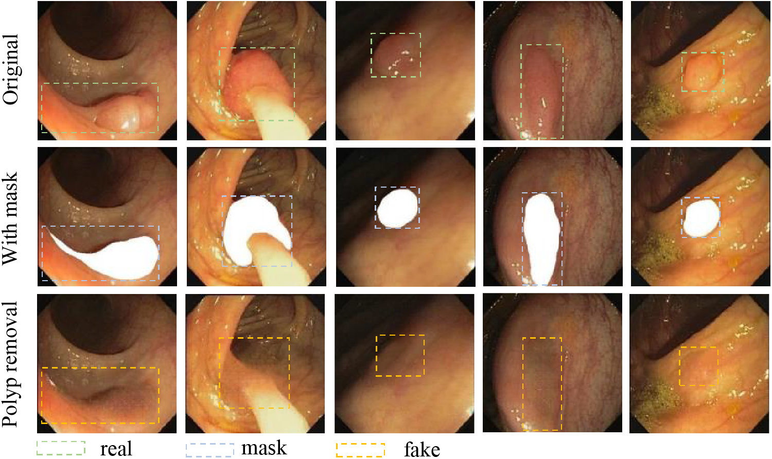
Figure 10: Polyp elimination reasoning images

3.3.2 Polyp Generation Reasoning

In this task, the way we set up our polyp mask has changed. First, we extracted polyp masks from existing real images. Next, a region in the image where polyps need to be generated is extracted based on its color features where polyps are likely to be present. Finally, we superimposed the fusion of that polyp mask at random locations within that region using the OpenCV algorithm, as shown in the second column of Fig. 11. We utilized the polyp generation weights to reason about the set mask image. This results in a new polyp sample. While the polyp images generated with the original masks contain rich color information, they lack new edge details. This leads to saturation in the information provided by the dataset, meaning that as more samples are generated, the dataset’s potential for improving detection performance will plateau. However, using randomly angled overlays for mask generation introduces rich edge details, helping us address this issue. The mask setup method we used was to set the target region in the sample using the OpenCV algorithm. Randomly pair 2 to 3 masks in the extracted masks and set random angles to superimpose them. The superimposed image is shown in the second column of Fig. 12. As shown in the third column of Figs. 11 and 12, the random superposition of masks generates richer polyp shapes, which can effectively solve the problem of limited performance of the detection model due to a single polyp shape.

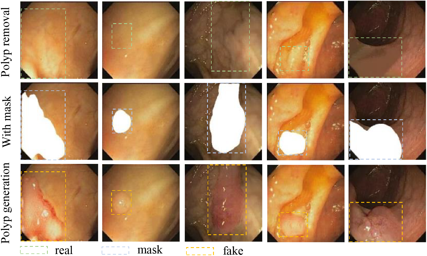
Figure 11: Polyp generation reasoning images

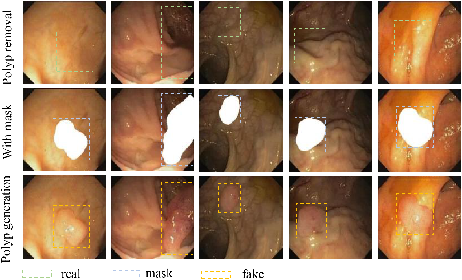
Figure 12: Polyp images generation using random combination masks

3.4 WGAN-GP Validity Verification

Training unstable has always been a problem for GAN, whereas the existence of WGAN-GP makes our generative model more stable and thus performs better generative performance. As proof of the effectiveness of WGAN-GP, we compared the training using three loss algorithms Least Squares GAN (Lsgan) [21], Vanilla [5] and WGAN-GP. The results are shown in Fig. 13, the model using WGAN-GP reaches stability at 100 epochs. Its faster convergence and lower loss value compared to the model using Lsgan and Vanilla loss, which allows our generative model to perform better.

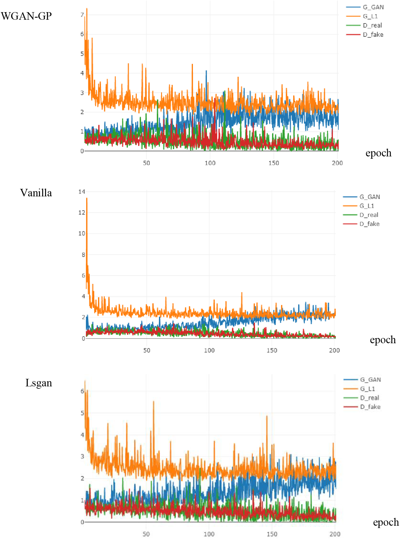
Figure 13: Loss curves of different algorithms

3.5 Evaluation Metrics

Aiming at evaluating the role of the attention mechanism in image generation, we mainly use two commonly used evaluation metrics, peak signal-to-noise ratio (PSNR), structural similarity index (SSIM) and mean squared error (MSE). These evaluation metrics are often used to assess the similarity of images. We test the effectiveness of the attention mechanism by comparing these two metrics in image generation.

The PSNR calculation formula is shown in Eq. (5):

PSNR=10⋅log10(MAX2MSE)(5)

PSNR is an important indicator of the generated image, MAX represents the maximum value of the information of the generated data, and MSE represents the mean square error of the generated data, so the smaller the MSE is, the larger the PSNR is; the larger the PSNR is, the better the quality of the reconstructed image is represented.

SSIM(x,y)=(2μxμy+c1)(2σxy+c2)(μx2+μy2+c1)(σx2+σy2+c2)(6)

SSIM is shown in Eq. (6), which is calculated based on the comparison of three important indexes: brightness, contrast and structure of two image data, the larger SSIM means the better image quality, the limit value is 1, x is the generated false data, y is the real labeled data, μx and μy are the mean value of x and y, respectively. σx2 and σy2 are the covariance of x, y, respectively. c1 as well as c2 are 2 constants.

MSE is a commonly used indicator to measure the degree of difference between predicted and actual values. It calculates the mean square of the difference between predicted and actual values. The smaller the MSE value, the better the prediction performance of the prediction model. The formula for MSE is shown in Eq. (7), where n is the number of samples, Yi is the actual value of the i-th sample, and Y^i is the predicted value of the i-th sample.

MSE=1n∑i=1n(Yi−Y^i)2(7)

To compare the detection performance of our proposed dataset with that of other datasets used in target detection studies, we employ the same evaluation metrics as those utilized by the authors of previous papers. These metrics include true positives (TP), false positives (FP), false negatives (FN), and true negatives (TN). In this context, TP refers to the correct detection of polyps, while FP indicates false detections, with negative samples incorrectly predicted as positive. Furthermore, FN represents missed detections of polyps, in which positive samples are predicted as negative, and TN denotes the correct identification of negative samples. From this, we know that for target detection, the larger TP and TN are, the better the performance of this target detection model is demonstrated, and the smaller FP and FN are, the better the model performance is demonstrated. Based on these four parameters, we also designed three additional evaluation metrics, namely precision (Pre), recall (Rec) and f1-score (f1).

Pre=TPTP+FP×100(8)

Rec=TPTP+FN×100(9)

f1=2×Rec×PreRec+Pre×100(10)

J(A,B)=|A∩B||A∪B|=|A∩B||A|+|B|−|A∩B|(11)

Dice(A,B)=2|A∩B||A|+|B|(12)

In terms of comparing our performance on segmentation with the dataset proposed by others, we mainly used the Jaccard index (J) and Dice similarity score (Dice), both of which are formulated as shown in Eqs. (11) and (12). Where A refers to the segmentation result predicted by the model and B refers to the true segmentation result corresponding to A.

3.6 Experiments on Attention Mechanisms

The attentional mechanisms in the generative model can help us to eliminate interference. To further validate their effectiveness, we placed the two attention mechanisms in the generator part of the generative model as shown in Fig. 2. In addition, to examine the effect of different attention mechanisms on the model generation results, we conducted ablation experiments on different down-sampling levels and numbers of the attention mechanisms in the U-Net generator as shown in Table 1. The experimental results demonstrate that the generated model is improved to a small extent after adding the attention mechanism. Among them, the best generation effect is achieved when CA is placed in the first, second and third layers of the U-Net network at the same time. Its PSNR reached 33.9737, SSIM reached 0.9809 and MSE reached 25.9855. This indicates that the image generated by placing Ca in this position will be more similar to the real image. Therefore, this attention-setting method can make the generation model play the best performance. This is why we chose this setting method.

Besides, we conducted heatmap analysis on images generated without attention and those with attention added at the optimal position. As shown in Fig. 14, A1 and B1 represent the polyp images generated before and after the addition of the attention mechanism, respectively. A2 and B2 are their respective heat maps. As shown in this image, the model without attention disperses focus on reflective areas and generates content there. This hinders the generation of high-quality polyp samples. With attention added, the model dynamically adjusts weights across regions. It concentrates on the target area and suppresses reflective parts. This helps the model avoid interference from reflections. Therefore, adding attention aids in generating high-quality polyp samples.

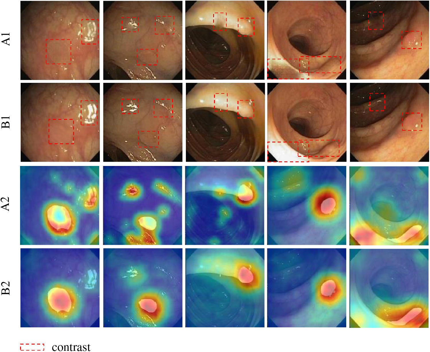
Figure 14: Visual experiment. A2 and B2 are the heat map displays of A1 and B1, respectively

3.7 Object Detection Performance Comparison

So as to be able to demonstrate more directly the superiority of our generated dataset on the target detection model, we compared it with the datasets generated by [10,18], and [9] under the same conditions. Where [18] represents a data set composed of original images. We will compare on Faster R-CNN ResNet101, Faster R-CNN Inception Resnet v2 and R-FCN ResNet101. The results are shown in Tables 2–4.

As can be seen from the data in these tables, in comparison with the original dataset and the dataset proposed by others, although our dataset is slightly inferior in some of the metrics, it improves and optimizes the three important performance metrics of Pre, Rec, and f1. This indicates that our dataset can help the object detection model learn more features, thereby improving the performance of the detection model. In the first experiment, the dataset we generated achieved 68.1%, 86.91%, and 76.36% on Rec, Pre, and f1 metrics, respectively. In the second experiment, the dataset we generated achieved 72.91%, 85.78%, and 78.82% on Rec, Pre, and f1 metrics, respectively. In the third experiment, the dataset we generated achieved 66.72%, 89.34%, and 76.39% on Rec, Pre, and f1 metrics. It follows that it can be seen that the performance of our improved generative model is superior to the generative models proposed by other scholars.

3.8 Segmentation Performance Comparison

In order to better demonstrate the superior performance of our generated datasets on the segmentation task, we compare them on a range of segmentation metrics under the same conditions. Table 5 demonstrates the performance comparison of the three types of segmentation models. The comparison is for the initial dataset, which is a dataset of 612 images without any generated images. In addition, the dataset proposed by other scholars and the dataset generated by us are also included. Where reference [9] is the original dataset plus 372 generated polyps, reference [10] is the original dataset plus 350 generated polyps, and our expanded dataset is the original dataset plus 350 generated polyps.

The results obtained are shown in Table 5. Upon training with our dataset, its performance is superior on all three segmentation models. TernausNet-16 improves by 8.72% and 11.06% on the Jaccard and Dice metrics respectively, reaching the best in its group. AlbuNet-34 improves by 4.49% and 7.91% on the Jaccard and Dice metrics respectively, reaching the best in its group. MDeNetplus is the best in its group with an improvement of 6.19% and 8.83% on the Jaccard and Dice metrics, respectively. The experimental results of the three segmentation methods show that our generated dataset exhibits the best segmentation performance. This finding further highlights the superiority of our generation algorithm.

3.9 Comparison of Polyp Datasets Generated Using Different Masks

In an effort to demonstrate the effectiveness of using different masks to generate diverse polyps and enhance the performance of various models on the dataset, we conducted a comparative analysis using the object detection model R-FCN ResNet101. This analysis provided us with the opportunity to assess the impact of our approach on model performance. As shown in Fig. 15, black represents the polyp dataset generated without adding the mixed mask, red represents the polyp dataset generated by mixing the old and new masks in a 1:1 ratio, and the y-axis represents the number of newly generated images added. As shown in the figure, the dataset without polyps of different shapes reached saturation performance after adding 350 images. The performance indicators of the dataset with mixed polyp images are still improving.

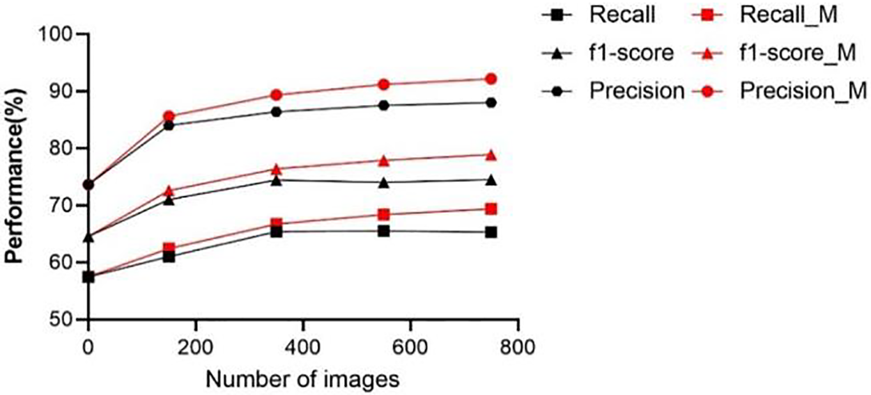
Figure 15: Performance comparison of data sets generated by different mask schemes

4  Conclusion

Polyp datasets are more challenging to collect and process compared to general datasets. To address these challenges, we designed a Pix2Pix-based polyp image generation scheme to address a series of difficulties. In this scheme, we utilized the same model to achieve polyp elimination and generation. For the interference and other factors in the image, we designed the attention mechanism module, which resulted in a notable improvement in the image production index. Simultaneously, we discovered during testing that utilizing the original polyp mask for polyp generation would stagnate the subsequent detection performance. Therefore, we randomly mixed different masks to generate polyp images with different feature information. In this regard, we have conducted a series of experiments to verify the feasibility of our proposed scheme. However, during the completion of the polyp generation task, we faced another major challenge, the low resolution of the generated polyp images. In the next step, we will conduct further research with the goal of improving the resolution of the generated images.

Acknowledgement: The authors would like to express our sincere gratitude and appreciation to each other for our combined efforts and contributions throughout the course of this research paper.

Funding Statement: This project was supported by the Natural Science Foundation Project of Fujian Province, China (Grant Nos. 2023J011439 and 2019J01859).

Author Contributions: The authors confirm contribution to the paper as follows: Study conception and design: Ziji Xiao, Kaibo Yang, Mingen Zhong; data collection: Ziji Xiao, Kaibo Yang; analysis and interpretation of results: Ziji Xiao, Kaibo Yang, Jiawei Tan, Kang Fan; draft manuscript preparation: Ziji Xiao, Zhiying Deng. All authors reviewed the results and approved the final version of the manuscript.

Availability of Data and Materials: The data used to support the findings of this study are available from the corresponding author upon request. Datasets are available at: https://polyp.grand-challenge.org/ (accessed on 10 May 2024). All datasets are publicly accessible.

Ethics Approval: Not applicable.

Conflicts of Interest: The authors declare no conflicts of interest to report regarding the present study.

References

1. G. Ciuti et al., “Frontiers of robotic endoscopic capsules: A review,” J. Micro-Bio Robot, vol. 11, no. 1–4, pp. 1–18, 2016. doi: 10.1007/s12213-016-0087-x. [Google Scholar] [PubMed] [CrossRef]

2. M. B. Wallace et al., “Impact of artificial intelligence on miss rate of colorectal neoplasia,” Gastroenterology, vol. 163, no. 1, pp. 295–304, 2022. doi: 10.1053/j.gastro.2022.03.007. [Google Scholar] [PubMed] [CrossRef]

3. S. M. A. Sharif, R. A. Naqvi, Z. Mehmood, J. Hussain, A. Ali and S. -W. Lee, “MedDeblur: Medical image deblurring with residual dense spatial-asymmetric attention,” Mathematics, vol. 11, no. 1, 2023, Art. no. 115. doi: 10.3390/math11010115. [Google Scholar] [CrossRef]

4. S. M. A. Sharif, R. A. Naqvi, F. Ali, and M. Biswas, “DarkDeblur: Learning single-shot image deblurring in low-light condition,” Expert. Syst. Appl., vol. 222, no. 1, 2023, Art. no. 119739. doi: 10.1016/j.eswa.2023.119739. [Google Scholar] [CrossRef]

5. I. Goodfellow et al., “Generative adversarial networks,” Commun. ACM, vol. 63, no. 11, pp. 139–144, 2020. doi: 10.1145/3422622. [Google Scholar] [CrossRef]

6. F. Calimeri, A. Marzullo, C. Stamile, and G. Terracina, “Biomedical data augmentation using generative adversarial neural networks,” in Artificial Neural Networks and Machine Learning–ICANN 2017. Cham: Springer, 2017. doi: 10.1007/978-3-319-68612-7_71. [Google Scholar] [CrossRef]

7. M. V. Golhar, T. L. Bobrow, S. Ngamruengphong, and N. J. Durr, “GAN inversion for data augmentation to improve colonoscopy lesion classification,” IEEE J. Biomed. Health Inform., 2024. doi: 10.1109/JBHI.2024.3397611. [Google Scholar] [PubMed] [CrossRef]

8. V. de Almeida Thomaz, C. A. Sierra-Franco, and A. B. Raposo, “Training data enhancements for improving colonic polyp detection using deep convolutional neural networks,” Artif. Intell. Med., vol. 111, no. 6, 2021, Art. no. 101988. doi: 10.1016/j.artmed.2020.101988. [Google Scholar] [PubMed] [CrossRef]

9. Y. Shin, H. A. Qadir, and I. Balasingham, “Abnormal colon polyp image synthesis using conditional adversarial networks for improved detection performance,” IEEE Access, vol. 6, pp. 56007–56017, 2018. doi: 10.1109/ACCESS.2018.2872717. [Google Scholar] [CrossRef]

10. H. A. Qadir, I. Balasingham, and Y. Shin, “Simple U-net based synthetic polyp image generation: Polyp to negative and negative to polyp,” Biomed. Signal Process. Control, vol. 74, no. 6, 2022, Art. no. 103491. doi: 10.1016/j.bspc.2022.103491. [Google Scholar] [CrossRef]

11. P. Isola, J. Y. Zhu, T. Zhou, and A. A. Efros, “Image-to-image translation with conditional adversarial networks,” in Proc. 30th IEEE Conf. Comput. Vis. Pattern Recognit., CVPR 2017, 2017. doi: 10.1109/CVPR.2017.632. [Google Scholar] [CrossRef]

12. I. Gulrajani, F. Ahmed, M. Arjovsky, V. Dumoulin, and A. Courville, “Improved training of wasserstein GANs,” in 31st Annu. Conf. Neural Inform. Process. Syst. (NIPS 2017), Long Beach, CA, USA, 2017. [Google Scholar]

13. M. Arjovsky, S. Chintala, and L. Bottou, “Wasserstein GAN martin,” 2017, arXiv:1701.07875. [Google Scholar]

14. S. Ren, K. He, R. Girshick, and J. Sun, “Faster R-CNN: Towards real-time object detection with region proposal networks,” IEEE Trans. Pattern Anal. Mach. Intell., vol. 39, no. 6, pp. 1137–1149, 2017. doi: 10.1109/TPAMI.2016.2577031. [Google Scholar] [PubMed] [CrossRef]

15. J. Dai, Y. Li, K. He, and J. Sun, “R-FCN: Object detection via region-based fully convolutional networks,” in 30th Annu. Conf. Neural Inform. Process. Syst. (NIPS 2016Barcelona, Spain, 2016. [Google Scholar]

16. V. Iglovikov and A. Shvets, “TernausNet: U-Net with VGG11 encoder pre-trained on imagenet for image segmentation,” 2018, arXiv:1801.05746. [Google Scholar]

17. H. A. Qadir, Y. Shin, J. Solhusvik, J. Bergsland, L. Aabakken and I. Balasingham, “Toward real-time polyp detection using fully CNNs for 2D Gaussian shapes prediction,” Med. Image Anal., vol. 68, no. 4, 2021, Art. no. 101897. doi: 10.1016/j.media.2020.101897. [Google Scholar] [PubMed] [CrossRef]

18. J. Bernal, F. J. Sánchez, G. Fernández-Esparrach, D. Gil, C. Rodríguez and F. Vilariño, “WM-DOVA maps for accurate polyp highlighting in colonoscopy: Validation vs. saliency maps from physicians,” Comput. Med. Imaging Graph, vol. 43, no. 1258, pp. 99–111, 2015. doi: 10.1016/j.compmedimag.2015.02.007. [Google Scholar] [PubMed] [CrossRef]

19. J. Silva, A. Histace, O. Romain, X. Dray, and B. Granado, “Toward embedded detection of polyps in WCE images for early diagnosis of colorectal cancer,” Int. J. Comput. Assist Radiol Surg., vol. 9, no. 2, pp. 283–293, 2014. doi: 10.1007/s11548-013-0926-3. [Google Scholar] [PubMed] [CrossRef]

20. Q. Angermann et al., “Towards real-time polyp detection in colonoscopy videos: Adapting still frame-based methodologies for video sequences analysis,” in Computer Assisted and Robotic Endoscopy and Clinical Image-Based Procedures. Cham: Springer, 2017. doi: 10.1007/978-3-319-67543-5_3. [Google Scholar] [CrossRef]

21. X. Mao, Q. Li, H. Xie, R. Y. K. Lau, Z. Wang and S. P. Smolley, “Least squares generative adversarial networks,” in Proc. IEEE Int. Conf. Comput. Vis., 2017. doi: 10.1109/ICCV.2017.304. [Google Scholar] [CrossRef]