
 Submit a Paper
 Propose a Special lssue
 Open Access
ARTICLE

kProtoClust: Towards Adaptive k-Prototype Clustering without Known k
1 School of Information Engineering, Xuchang University, Xuchang, 461000, China
2 Henan Province Engineering Technology Research Center of Big Data Security and Applications, Xuchang, 461000, China
3 College of Computer Science and Technology, Guizhou University, Guiyang, 550025, China
4 Here Data Technology, Shenzhen, 518000, China
* Corresponding Author: Yuan Ping. Email:
Computers, Materials & Continua 2025, 82(3), 4949-4976. https://doi.org/10.32604/cmc.2025.057693
Received 25 August 2024; Accepted 16 December 2024; Issue published 06 March 2025
 View Full Text
 Download PDF
Abstract
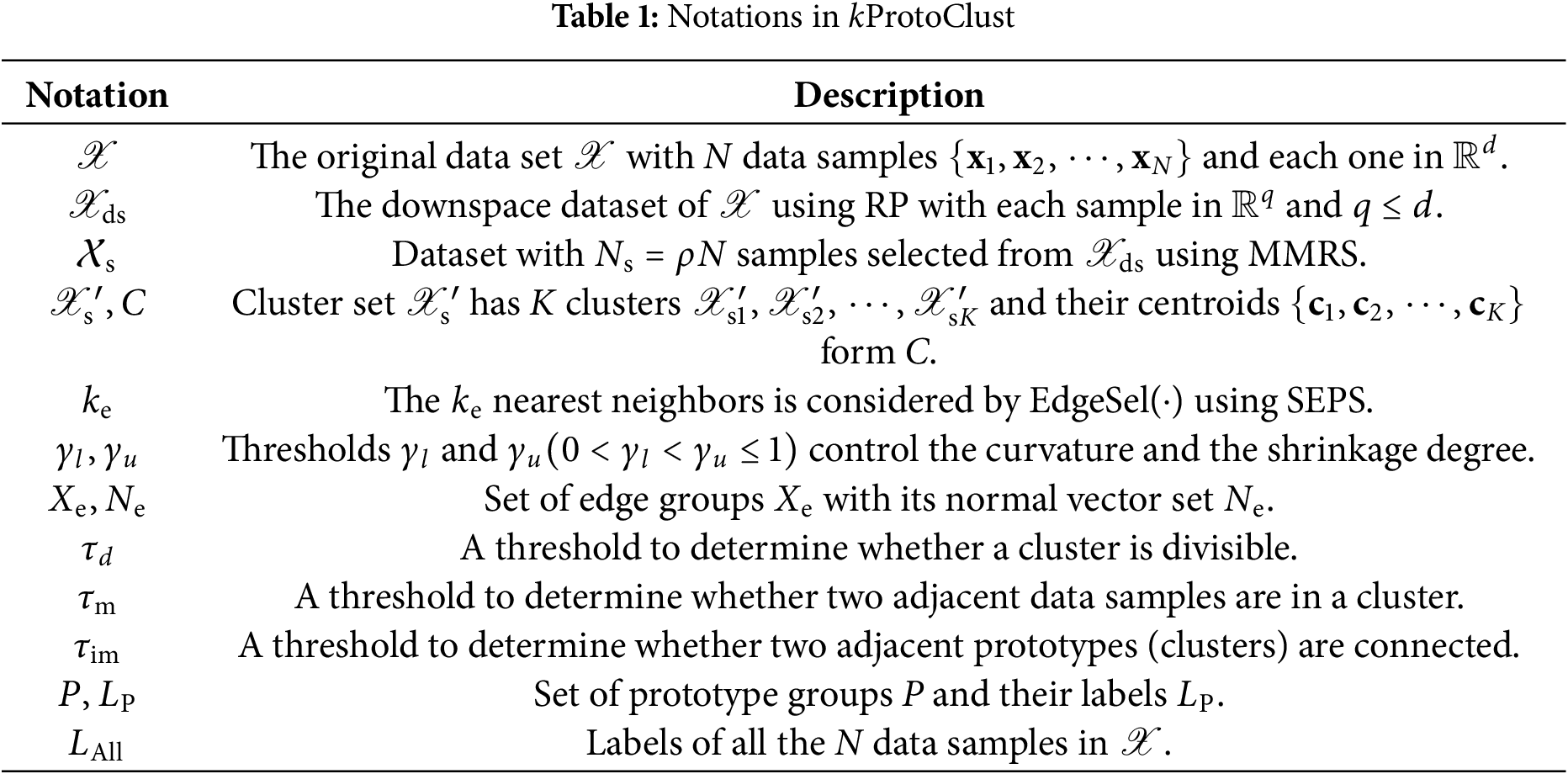
Towards optimal k-prototype discovery, k-means-like algorithms give us inspirations of central samples collection, yet the unstable seed samples selection, the hypothesis of a circle-like pattern, and the unknown K are still challenges, particularly for non-predetermined data patterns. We propose an adaptive k-prototype clustering method (kProtoClust) which launches cluster exploration with a sketchy division of K clusters and finds evidence for splitting and merging. On behalf of a group of data samples, support vectors and outliers from the perspective of support vector data description are not the appropriate candidates for prototypes, while inner samples become the first candidates for instability reduction of seeds. Different from the representation of samples in traditional, we extend sample selection by encouraging fictitious samples to emphasize the representativeness of patterns. To get out of the circle-like pattern limitation, we introduce a convex decomposition-based strategy of one-cluster-multiple-prototypes in which convex hulls of varying sizes are prototypes, and accurate connection analysis makes the support of arbitrary cluster shapes possible. Inspired by geometry, the three presented strategies make kProtoClust bypassing the K dependence well with the global and local position relationship analysis for data samples. Experimental results on twelve datasets of irregular cluster shape or high dimension suggest that kProtoClust handles arbitrary cluster shapes with prominent accuracy even without the prior knowledge K.Keywords
Clustering is to discover natural data groups with maximal intra-cluster similarity yet minimal inter-cluster similarity. As one of the most well known algorithms, k-means adopts an iterative strategy with conditional termination, in which labeling each data sample to the nearest cluster centroid and recalculating the centroids are alternately conducted. Due to insufficient prior knowledge, discovering data groups is an exploration procedure toward the target data. First, a predefined K is frequently impractical before we judge the exact distribution pattern, e.g., customer segmentation, and anomaly detection [1,2]. Second, k-means ultimately does input space partition insensitive to the data distribution boundary. Therefore, a data set can be partitioned differently, and the random selection of initial cluster centroids can aggravate ineradicable instability. Third, under the K constraint, partitioning input space in terms of circle-like patterns requires further exploration to deal with arbitrary cluster shapes.
Considering the challenges above, many insightful works can be found in the literature. Without the prior knowledge of K, two representative methods are distance-based and vote-based analysis after running k-means for a range of K values (e.g., 5–20). For the former, elbow curve and silhouette coefficient analysis [3] are two typical methods. For each K, elbow curve analysis calculates average distances to the centroid across all data samples and finds the point where the average distance from the centroid falls suddenly. Unlike elbow curve analysis, silhouette coefficient analysis measures how similar a data sample is within a cluster (cohesion) compared to other clusters (separation). An average score on each K will be obtained before making a judgment. Besides, authors in [4] introduce enhanced gap statistic (EGS) to measure the standardized difference between the log-transformed within-cluster sums of squares from a reference dataset of exponential distribution. A better K should reduce the variation. For the latter, Fred et al. [5] suggest evidence accumulation (EAC) to combine multiple results under a vote strategy. It works well in identifying arbitrarily shaped cluster, particularly on low-dimensional data with clear boundaries. Since the initialization phase strongly influences the obtained accuracy and computational load, a common sense of coping strategy is to restart k-means several times under one of seeding strategies and keep the final result with the lowest error. Besides the random seeding strategy employed by the classic k-means, the other popular strategies include Forgy’s approach [6], probabilistic-based strategy [7,8], and the most recent split-merge approach [9]. For k-means and its variants, the circle-like pattern hypothesis is preserved. Therefore, split-merge [5,9], multiprototype [10], and multiple kernels-based strategy [11] are mainly adopted for imbalanced clusters. In addition, the outlier removal matching k-means is getting more attention for accuracy. Despite the above representative methods making improvements on accuracy, efficiency or adaptability for k-means, the requirement of K approximating the ground truth is almost kept. Furthermore, even if K is given, the intrinsic input space division strategy and the circle-like pattern hypothesis also can not match irregular cluster shapes [9], since they should be considered along with the exploration of unknown K clusters.
Despite challenges, k-means inspires us for its simplicity, intuition, and efficiency. In this paper, an adaptive k-prototype clustering namely kProtoClust is designed to cast off the K dependence, optimize seeds extraction, and reduce the influence from circle-like pattern description. The discovered clusters can change in number and shape and become apparent along with the global and local position relationship analysis. The main contributions of this work lie in:
(1) Inspired by the concept of support vector data description (SVDD), convex hulls of variable sizes described by boundary patterns [12] are employed as prototypes. Discarding the circle-like pattern assumption, kProtoClust is never an input space division method but a boundary discovery-based clustering method with a convex decomposition strategy that prefers one-cluster-multiple-prototypes. Thus, arbitrary-shaped clusters can be well discovered and described.
(2) K is no longer an objective for input space division but a starting point for cluster exploration. Based on a union analysis of the global and local position relationship for data samples, we find solid evidence for split and mergence. Begin with an initial K for a sketchy division of input space, kProtoClust discovers optimal clusters in accord with data distribution. The prior knowledge K is bypassed due to giving no constraint on the final cluster number
(3) To reduce redundant computations, we propose a careful seeding strategy with position analysis (S2PA) in which a lightweight data grouping algorithm and logical inner analysis are carefully introduced. It gets two critical yet intuitive features: K seeds selection must evade outliers and boundaries and should not be limited to existing samples in the target data. As an assistant of kProtoClust in an early collection of cluster centers, k-means++ with S2PA contributes to accurate prototype analysis in stability and efficiency.
(4) By integrating the aforementioned designs, kProtoClust is proposed to achieve a better understanding of clusters from the basic component of convex hull. For efficiency, complete cluster exploration is conducted in input space. Furthermore, to reduce the impact of sparse data space on separability, a near maximin and random sampling (NMMRS) [13] is recommended for large and high dimensional dataset. More exploration spirits with the descriptive ability can be found in kProtoClust that motivates it to discover the accurate data distribution, not to divide the input data space under an inflexible rule. Compared with k-means-like algorithms [14], the cost of a slight efficiency drop is acceptable in practical data analysis.
The remainder of this paper proceeds as follows. Section 2 gives preliminaries of k-means++, SVDD, shrinkable edge pattern selection, and NMMRS. Section 3 describes the proposed kProtoClust with its critical components, e.g., S2PA, evidence of split and mergence, and convex decomposition based prototypes extraction. Section 4 evaluates the performance of kProtoClust. In Section 5, we discuss related work. In Section 6, we conclude this work.
Consider a data set
Generally, k-means++ selects the first center
Here,
2.2 Support Vector Data Description
Giving a nonlinear function
where
with
2.3 Shrinkable Edge Pattern Selection
As depicted by Fig. 1, in geometrical, a cluster’s boundary consists of an edge and a border [16]. An edge belongs to one cluster, while a border appears in an overlapping region and is shared by two adjacent clusters which are generally considered as two components with the same cluster label. However, in unsupervised learning, it is difficult to find the border. Therefore, similar to SVDD, the edge contains the most informative samples that accurately describe the distribution structure. From this perspective, it can be considered a superset of SVs. In line with [12], the critical steps of shrinkable edge pattern selection (SEPS) for a given
• Setting two thresholds
• Generating the normal vector
• Calculating
• Cluster boundary identification. If
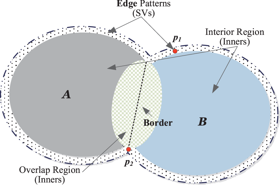
Figure 1: Edge patterns and border
2.4 Near Maximin & Random Sampling
Desired from the maximin sampling rule, NMMRS focuses on accurately portraying the distribution of
• Step 1: Collect
• Step 2: Group each data sample with its nearest maximin sample. By grouping each data sample in
• Step 3: Randomly select data near each maximin sample to obtain n samples. The final data
Towards discovering clusters without the ground truth, kProtoClust adopts edge-based cluster analysis since edges describe clusters and contribute to the connectivity analysis. Therefore, split analysis with S2PA given random seed K is designed to collect all the edge patterns forming convex hulls in local view. Mergence analysis tries to find the connectivity evidence of two neighboring convex hulls from a global view. In this section, we successively present the designs of edge collection, split and mergence analysis strategy, and finally give the algorithm description of kProtoClust.
3.1 Edges in Global and Local View
In kProtoClust, convex hulls with variable sizes are employed as the prototypes to support one-cluster-multiple-prototypes. From the perspective of SVDD following [12,17,18], the boundary is critical for convex hull extraction since the latter can be decomposed from the former. Even though a border is shared by two neighboring and connected convex hulls in the local view, it should be removed to accurately describe a cluster comprised of these two convex hulls in the global view. Therefore, although commonality exists, different perspectives frequently lead to very distinguished results. Without considering the border, the edge becomes the primary focus for kProtoClust.
Towards accurately and visually describing the difference between edges discovered in the global and local view, we consider one cluster with two prototypes (convex hulls) denoted by
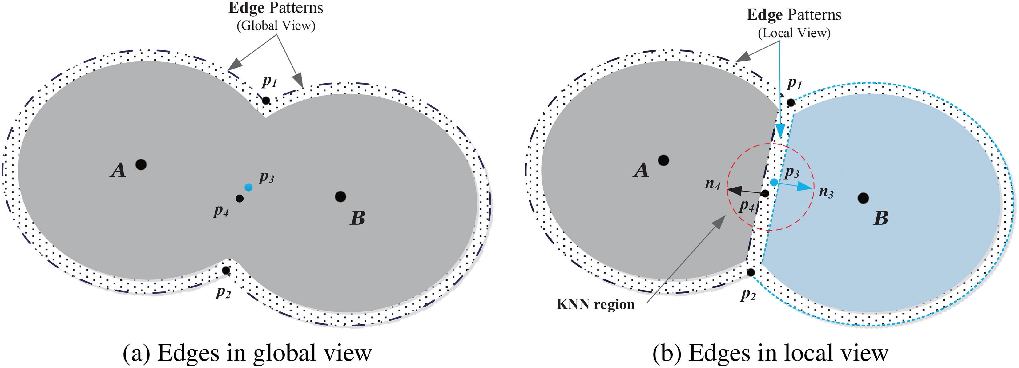
Figure 2: Edge analysis of two connected components in global and local view. In b), the two components are assigned with different labels after k-means++
Due to inaccurate data grouping or input space division, in the process of cluster exploration, inners like
Taking two irregularly shaped clusters Chameleon [19] as an example, edge patterns collected in a local view after k-means++ with
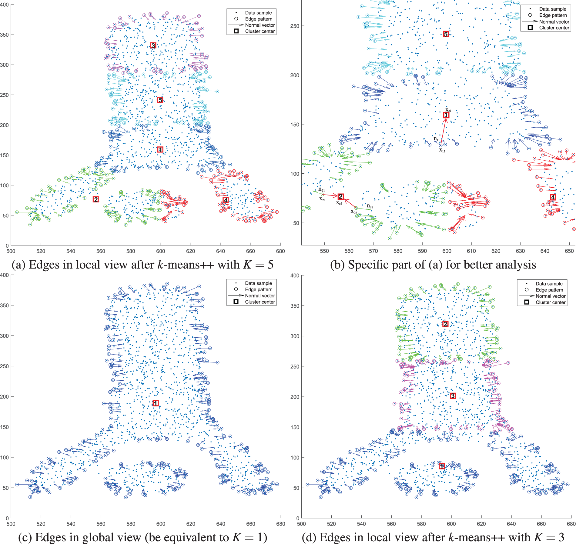
Figure 3: Edge analysis on two classes of Chameleon in global and local view with
The input space division strategy of k-means+ + allows us to efficiently observe data distribution patterns in a local view. Besides the separation of components of one cluster, components from different clusters can also be mistakenly grouped due to the circle-like hypothesis. As shown in Fig. 3a, cluster 2 covers two components that should be assigned with different labels. A similar result occurs in cluster 4. Before discovering the disconnection evidence, we first retrospect the convex hull definition following [17,20].
Definition 1 (convex hull). In Euclidean space, the convex hull of a data set
In
Proposition 1. For a convex hull
Proof. Based on Definition 1, there are
The numerator of Eq. (6) is
Meanwhile, due to
Based on the properties of convex hull and convex hull based decomposition [17], experimental result on Chameleon shown in Fig. 3b confirms the aforementioned two features.
• First, the center
• Second,
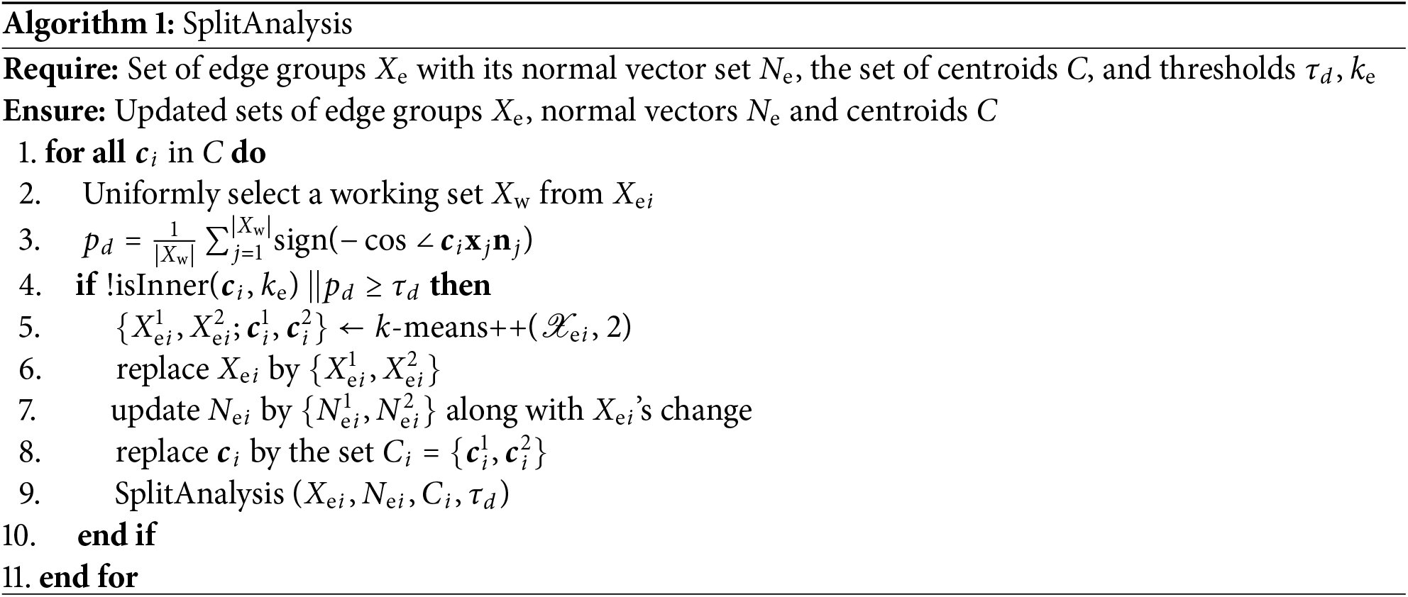
Based on the aforementioned S2PA strategy and violating sample analysis, an essential cluster split for mistake correction can be briefly illustrated in Algorithm 1. Given a set of edge pattern groups
where
According to the analysis in Section 3.1, violating samples exist in the overlapping region of two adjacent clusters or convex hulls. Therefore, as shown in Algorithm 2, the mergence analysis of convex hulls extracted by SplitAnalysis is quite intuitive: find out violating samples and merge the associated convex hulls to add prototypes for the corresponding cluster.
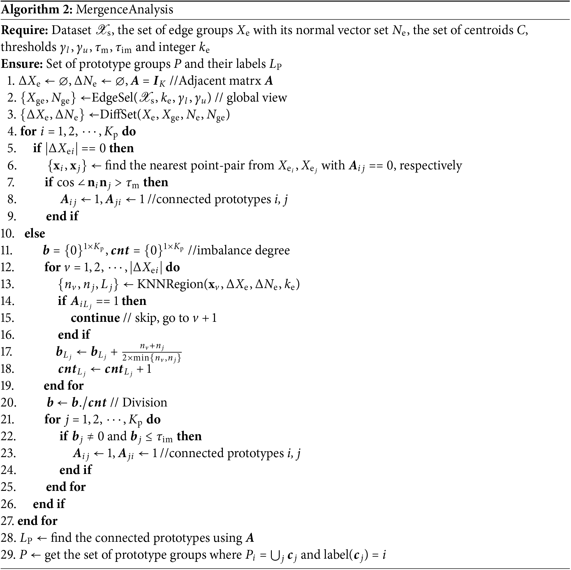
Algorithm 2 of MergenceAnalysis invokes EdgeSel(
If the current convex hull has no violating samples, lines 5–9 find two nearest edge patterns
Line 10 starts a series of distinguished works with violating samples in the current convex hull. Each KNN Region around the violating point will be carefully checked to obtain an accumulated imbalance for each adjacent prototype pair. When KNNRegion(
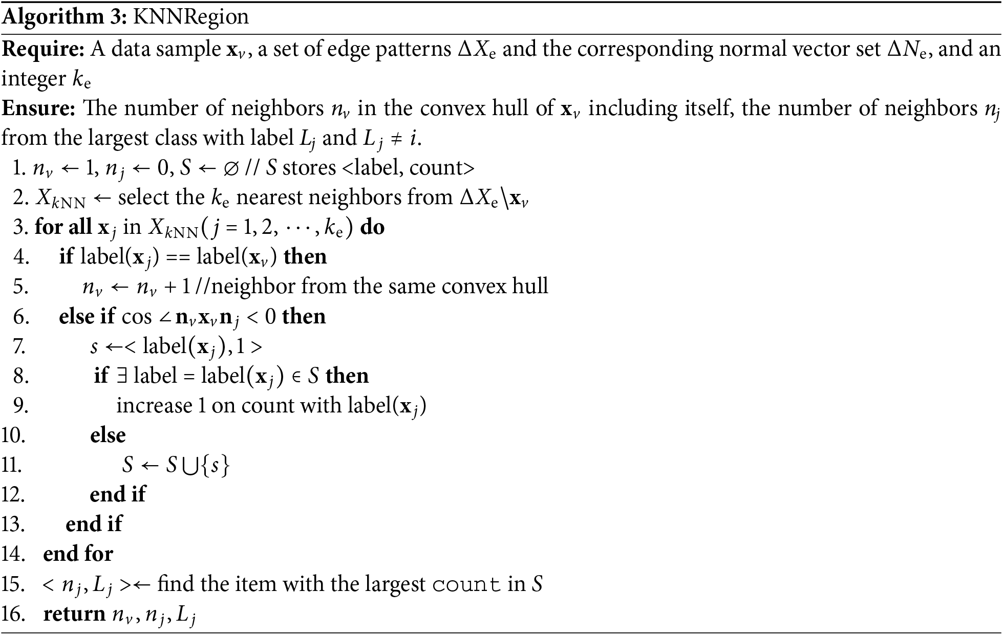
where only two different labels
3.4 Implementation of kProtoClust
Based on the split and mergence analysis, the proposed kProtoClust is detailed by Algorithm 4.
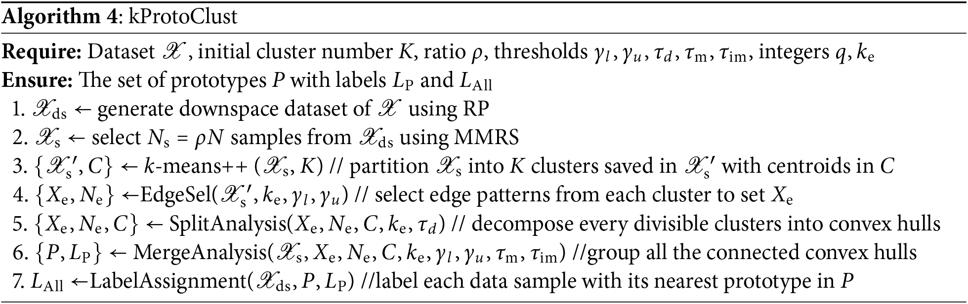
On the basis of keeping data distribution patterns, data sampling and dimension reduction are effective ways for efficiency. As data preparation works, however, they are frequently optional since only some of the data sets to be analyzed are large-scale with high dimensions. Therefore, Algorithm 4 prefers NMMRS [13] in lines 1–2 to make the following analysis done in the downspace if the target data is large-scale with high dimensions. Then, a standard k-means++ is employed to partition data into K clusters for further edge pattern selection in the local view. Since the difference of edge patterns collected in terms of local and global views mainly lies in the border patterns, which are also inners in the perspective of SVDD. K is not a decisive prior knowledge. How to init the K value in the first round of line 3 only depends on the efficiency requirement from EdgeSel(
As shown in Algorithm 4, kProtoClust comprises six critical tasks. NMMRS consists of the first two lines yet optional data preparation works, as discussed in [13], which are suggested to be invoked if
Leaving NMMRS, k-means++ [7] costs
The overall computational complexity of kProtoClust is
4.1 Datasets and Experimental Settings
Inspired by a union analysis in the local and global view, kProtoClust provides adaptive multiple prototypes support while guaranteeing the fundamental principle of k-means. We conduct the following four series of experiments on various datasets to achieve a complete performance analysis.
• Do parameter sensitivity analysis on clustering accuracy and the discovered cluster number with respect to parameters K,
• Perform descriptive ability analysis for kProtoClust, in terms of accuracy, on classic datasets (type I in Table 2) with known cluster numbers. Since the foremost design of kProtoClust is to collect and well utilize the difference captured by local and global analysis, for fairness, we consider a compact version of kProtoClust including only lines 3–7 of Algorithm 4. Eight state-of-the-art algorithms are baselines:
• Check the cluster discovery ability of the compact kProtoClust on datasets of type I in Table 2 without the prior knowledge of cluster number
• Explore some applicable suggestions by verifying the effectiveness of kProtoClust with NMMRS (lines 1–2 of Algorithm 4) denoted by kProtoClust (RS) on datasets of type II in Table 2 which have either large number of samples or high dimensionality.
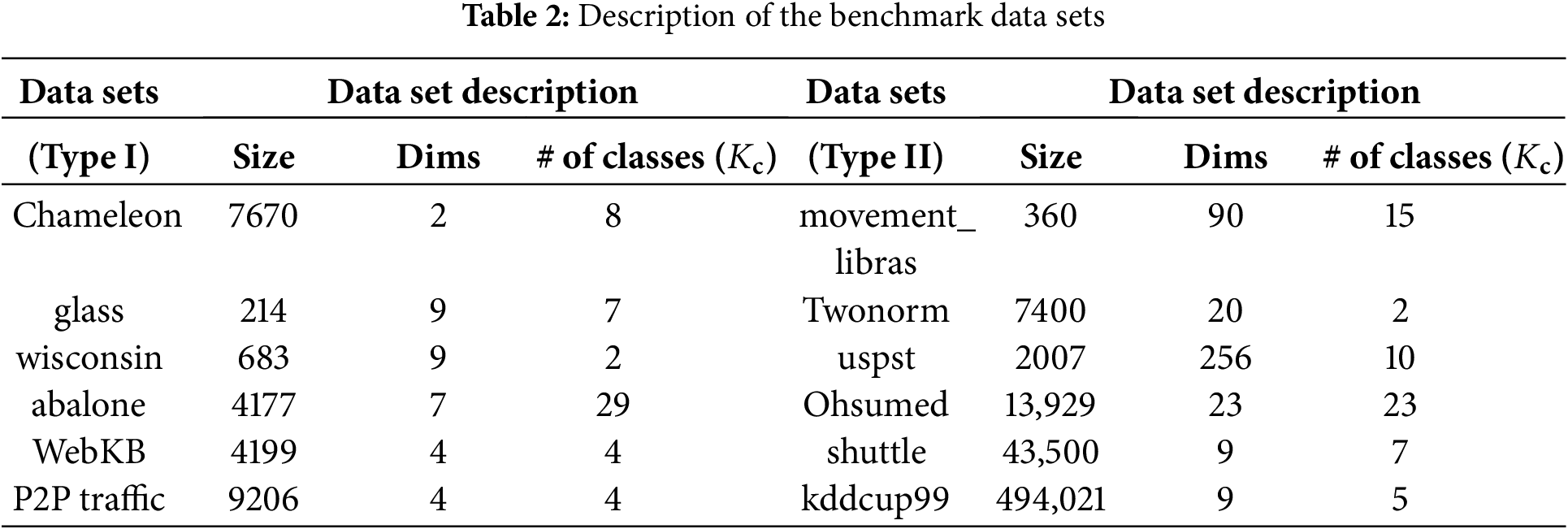
Table 2 lists the twelve employed datasets’ statistical information. Type I denotes small data with very irregular cluster shapes, while type II means more samples or higher dimensionality. They will be considered separately in different experiments to achieve a clear analysis. glass, wisconsin, abalone, movement_libras, Twonorm, uspst, and shuttle are from UCI repository [28]. WebKB [29] and Ohsumed [30] are pre-processed versions from [12]. Chameleon is provided by [19], and P2P traffic has 9206 flows’ features extracted by [31]. kddcup99 is a 9-dimensional data set extracted from KDD Cup 1999 Data [32] which is typical for intrusion detection. All the datasets are listed in the sequence of complexity
To evaluate the accuracy, adjusted rand index (ARI) [33], normalized mutual information (NMI) [34], and F-measure [35] are preferred. All the compared algorithms are implemented by MATLAB 2021b on a mobile workstation with Intel I9-9880H and 128 GB DRAM running Windows 10-X64. Since the main objectives are to verify the descriptive and cluster discovery abilities of the proposed kProtoClust, we do not pursue the maximal efficiency and the run-time is for limited reference.
4.2 Parameter Sensitivity Analysis
4.2.1 Initial Cluster Number K
Generally, unsupervised learning faces the critical challenge of lacking sufficient prior knowledge, such as the cluster number
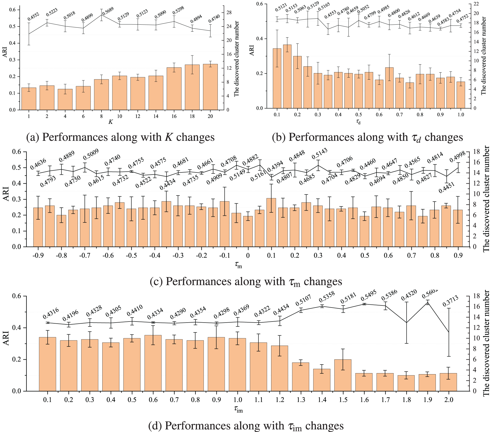
Figure 4: Sensitive analysis by means and standard variations of accuracy (ARI) and the cluster number (
4.2.2 Hyperparameters
Due to imbalanced distribution, non-accurate parameter settings in SEPS may miss some border patterns even though the nearest neighboring convex hulls are split from one cluster. To deal with this case,
In KNN region, the more balanced the edge patterns from different clusters are, the cumulative imbalance degree is close to
4.3 Performance Contrast with the Prior Knowledge Kc
The prior knowledge of cluster number is critical for k-means and its variants. Although kProtoClust is also derived from k-means, the design strategy of multiple prototypes support is to break through this constraint by emphasizing the descriptive ability. To verify the effectiveness, we compare it with twelve state-of-the-art methods on datasets of type I in terms of three accuracy metrics after thirty times of evaluations. The achieved mean and mean-square deviation (std) for each metric is illustrated in Table 3. Since descriptive ability is a common concern for all the methods considered from different perspectives, such as initialization strategy, data distribution description, or voting analysis, we omit efficiency comparisons for insignificant differences in low-complexity data despite having irregular clusters.
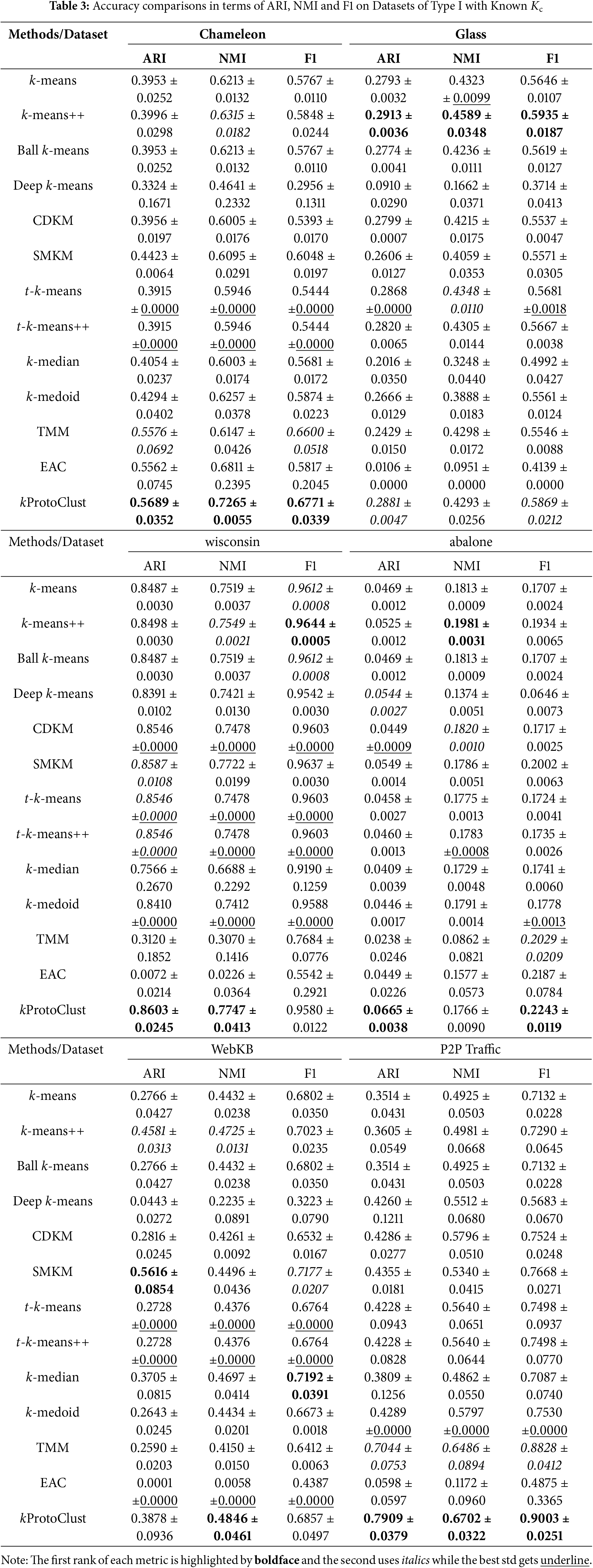
Consider data description in Table 2, we can get the following observations:
• Performances related to ARI, NMI, and F1 have similar trends for most cases. In terms of ARI, kProtoClust reaches the first rank on Chameleon, wisconsin, abalone, and P2P Traffic while performing the second on glass and the third on WebKB. Similarly, kProtoClust also reaches the best performance on four datasets in terms of NMI and on three data sets in terms of F1. Even though kProtoClust is not ranked first, it frequently gets into the first three ranks or obtains comparable accuracies. Relatively, kProtoClust has a significant advantage on datasets with small dimensions but more samples, e.g., Chameleon and P2P Traffic. Generally, in these cases, the more irregular the cluster shape is, the greater advantage it achieves.
• Besides kProtoClust, SMKM and k-means++ perform better than the others. They separately have the best ARI on glass and WebKB. Compared with k-means, coincidentally, they both achieve improvement by introducing the initialization strategy of centroid selection. k-means++ selects K centroids far away from each other, whereas SMKM introduces a cheap split-merge step to re-start k-means after reaching a fixed point. Compared with k-means++, SMKM has advantages on all the other five datasets. What follows is CDKM, which achieves comparable accuracies with SMKM and k-means++ yet performs more stable with much lower mean-square deviations.
• Unfortunately, there are no obvious advantages for Deep k-means, t-k-means, t-k-means++, and TMM, even though they tend to build distribution models for these datasets with extremely irregular cluster shapes. Similar performance can be found in k-means, Ball k-means, k-median, and k-medoid. Like CDKM, t-k-means and t-k-means++ have significant stability advantages due to pursuing the global optimization of Eq. (1). However, limited by the circle-like pattern hypothesis, global optimization usually does not mean the best cluster description for irregular shapes and imbalance distribution. Among these methods, EAC outperforms most of the others on low-dimensional datasets with clear shapes, e.g., Chameleon. However, noises and higher dimensions frequently make it fail, e.g., glass, wisconsin, WebKB, and P2P Traffic.
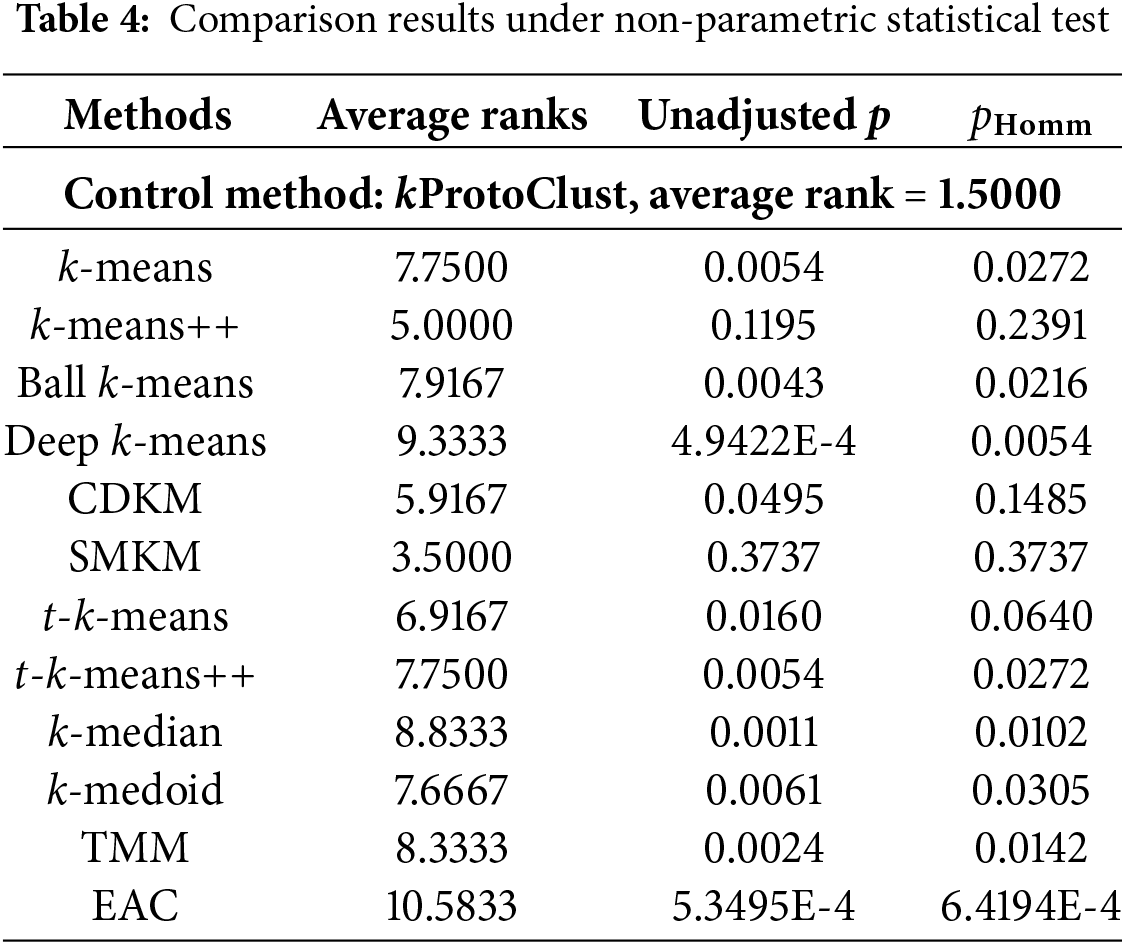
To further confirm the effectiveness of kProtoClust, we give results of pair comparisons in Table 4 following [37]. Taking kProtoClust as the control method, a typical nonparametric statistical test of Friedman test is adopted to get the average ranks and unadjusted p values. By introducing the Bergmann-Hommel procedure [38], the adjusted p-value denoted by
4.4 Exploration Contrast without the Prior Knowledge
For many real-world problems, e.g., intrusion behavior analysis, data owners can not have the prior knowledge
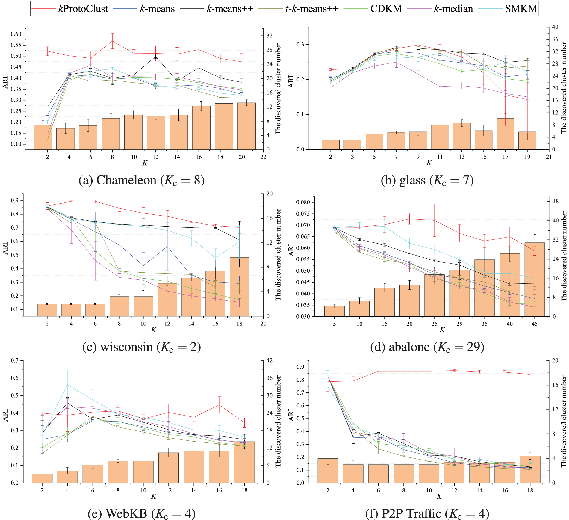
Figure 5: Accuracy (ARI) for all the compared methods and the cluster number found by kProtoClust without
Intuitively, without enough attention to the actual distribution, k-means, k-means++, and k-median try to do data division under different initialization strategies or distance measures. Although CDKM researches instability reduction by perusing the global optimization, t-k-means++ pays more attention to data distribution by introducing t-mixture distribution model, and SMKM adopts split-merge strategy to adjust clusters, they have to ensure the input space is divided into K clusters. Therefore, they can not avoid a severe deviation from the truth cluster number if we get an incorrect assumption of K. In contrast, the objective of split and merge analysis in kProtoClust is to dynamically generate an unfixed number of convex hulls of different sizes. Considering these convex hulls as prototypes, kProtoClust can better profile clusters with arbitrary shapes. Even though the discovered cluster number may not be equal to
Regarding ARI, the obtained accuracies show evidence of imbalanced distribution and irregular cluster shapes. For instance, accuracies obtained on Chameleon by the baseline methods are not falling off a cliff along with the increase of K, and the best accuracy on P2P Traffic is achieved when
Additionally, several other cues may be found from Fig. 5. First, for most cases, performances of baselines have specific decreases in accuracy when K is far from
4.5 Necessity Analysis of NMMRS for kProtoClust
Based on the analysis in Sections 3.5 and 4.4, when we fix the data size N, a greater dimensionality d not only increases its complexity but also reduces the separability. However, if d is fixed, the increase of N increases the complexity but will not permanently change (either increase or reduce) the separability. Therefore, we introduce NMMRS (lines 1–2 of Algorithm 4) into kProtoClust and denote it by kProtoClust(SR) in the following necessity analysis.
As discussed in Section 3.5, EdgeSel consumes
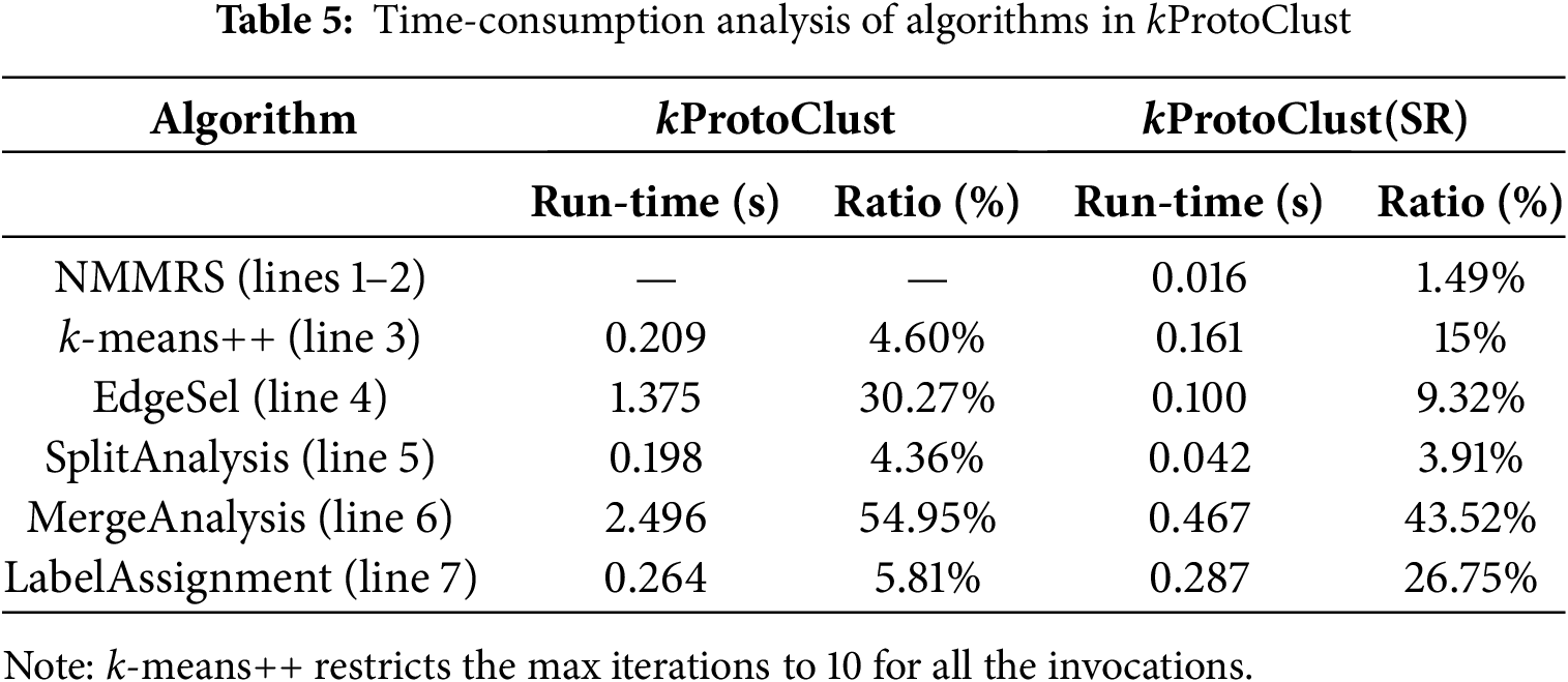
kProtoClust(SR) is a variant of k-means++ with split and mergence strategy. Meanwhile, SMKM also prefers a split-merge strategy and performs closely to kProtoClust(SR) in terms of accuracy on datasets of type I. In this section, we take k-means++ and SMKM as the baselines for further comparative analysis with kProtoClust and kProtoClust(SR). Results of accuracies in terms of ARI are depicted in Fig. 6 in which run-time costs required by kProtoClust and kProtoClust(SR) are also given. Due to
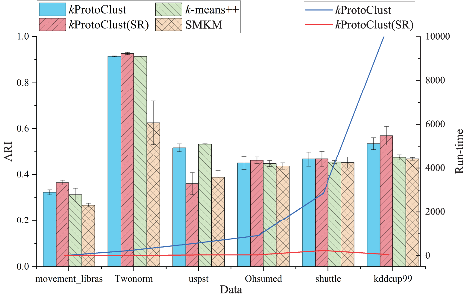
Figure 6: Performance analysis for kProtoClust with or without sampling and dimensionality reduction by taking k-means++ and SMKM as baselines.
In terms of efficiency, kProtoClust(SR) has a significant advantage over kProtoClust due to the introduction of NMMRS. On Twonorm, Ohsumed, shuttle and kddcup99, kProtoClust(SR) finish cluster analysis in 2.5, 40.7, 233.5 and 49.7 s, respectively. The run-time required by shuttle is greater than kddcup99 because the iterative analysis is more complex in SplitAnalysis (line 5 of Algorithm 4) due to extremely imbalanced distribution. Furthermore, results corresponding to all the datasets of type II confirm the contributions from NMMRS and suggest that the reduced dataset should have
k-means is the inspiration source of kProtoClust. Due to some intrinsic flaws inherited from the partition-based clustering strategy, the literature mainly focuses on further efficiency improvements, initialization strategy, stability optimization, and specific data types and patterns support.
The classical k-means selects K samples at random as the initial centroids and iteratively conducts the assignment and refinement until all the centroids do not change. For efficiency, besides hardware parallelization, fast convergence [7], result approximation [39], and distance computation reduction [14] are mainly focused. The last one receives the most attention for its generalization ability of computation optimization. Those representative works include avoiding unnecessary membership analysis by storing the different number of bounds for either centroids or data samples [40], and introducing group pruning and centroids regrouping strategy in the iteration [41]. For efficiency, Ryšavý et al. [42] makes a tighter centroid drift bound by employing the distance between the origin sample and the corresponding centroid, Bottesch et al. [43] adopts the Hölder’s inequality and norms, while Broder et al. [44] introduce a pre-assignment search around each centroid which greatly reduces distance computations. Recently, to optimize cluster assignment, Ball k-means [2] utilizes centroid distance. Besides, k-median [26] and k-medoid [27] can also be considered variants of k-means since the former introduces the Manhattan distance while the latter chooses existing data samples as centroids.
Many valuable solutions [45] corresponding to the initialization strategy, the main works are to estimate an appropriate K for centroids initialization. For the former, the mainstream way is parameter tweaking or evaluating models with different K settings [46] before finding out the usable K. Meanwhile, combining multiple clustering results with some voting strategies like EAC [5] or introducing some extensions of criterion such as Elbow index [47] are also considered. For the latter, besides pre-analysis of a set of potential centroids, Peña et al. [48] suggest that dividing a data set into K clusters and iteratively collecting K representative instances are practical. Furthermore, k-means++ [7] is a representative adopting the latter strategy since it chooses K centroids far away from each other.
Stability optimization is strongly related to the initialization strategy because the random initialization increases the instability. Recently, Capó et al. [9] present a split-merge strategy to restart k-means after reaching a fixed point. Therefore, their variant of k-means, namely SMKM, improves stability. However, multiple rounds of invocations to k-means and the split-merge strategy make it more suitable for dealing with clusters with irregular shapes. Another typical work in the most recently is CDKM [24], which designs a coordinate descent method for k-means to reach the global optimization of Eq. (1).
Different data types frequently relate to different application domains and distinct data patterns. In the literature, most works prefer doing special designs of k-means for a specific application. For instance, privacy-preserving k-means is presented for encrypted data analysis [49], global k-means based neural network performs well on sound source localization [50], while k-means with bagging neural network is suitable for short-term wind power forecasting [51]. Consider those mixed data types, the major attentions prefer fuzzy method [52], distance calculation mechanism [45], and hybrid framework [14]. Towards challenges from arbitrary cluster shapes, Li et al. [25] present t-k-means and t-k-means++ by assuming data sampled from the t-mixture distribution. Besides, Khan et al. [53] consider an exponential distribution to standardize data and propose EGS to estimate the optimal number of clusters. Fard et al. [23] present a joint solution namely deep k-means by integrating k-means and deep learning, while Peng et al. [54] adopt deep learning to re-describe k-means. Given the cluster number K, another exciting work [55] introduces k-means into SVDD such that it supports K groups of submodel of SVDD to describe different clusters in a data set. Lacking the prior knowledge of cluster number, EAC [5] clusters data with k-means based evidence accumulation. It conducts result combination with a specific vote strategy that well support low-dimensional data with clear and simple shape.
Despite many insightful works, they treat clusters fairly in size due to the limitation of the distance-based data partition. Few works change the initialized K in the clustering procedure. However, arbitrarily shaped clusters are very common in practice which motivates us to break the restriction of inaccurate prior-knowledge K and partition data into clusters with different sizes and connection relationships. Even though an optimal K is estimated by [53], utilizing K fixed clusters and K data samples as prototypes for label assignments can not match the human’s cognition of discovering clusters from their shapes, sizes, and connection relationships well. Therefore, kProtoClust takes convex hulls of varying sizes as prototypes following [17] and allows the change of K to support multiple prototypes in one cluster to improve cluster description ability.
With a specific distance measure, k-means find K data samples as prototypes to partition data space into clusters. However, not only the cluster number is unknown, but many practical datasets do not have a balanced and regular distribution as what k-means expected. To discover clusters following a general human cognition (corresponding to
Although kProtoClust achieves accuracy improvement with fair efficiency on datasets of imbalanced distribution and irregular cluster shapes, some shortcomings still exist, e.g., a certain instability inherited from k-means++. Meanwhile, the ways of handling high dimensional data with low separability and making the cluster number assessment more accurate are worthy of further investigation, as well as further improving the generalizability and adaptability across different scenarios, including semi-supervised clustering and clustering data streams.
Acknowledgment: We thank all the authors for their research contributions.
Funding Statement: This work is supported by the National Natural Science Foundation of China under Grant No. 62162009, the Key Technologies R&D Program of He’nan Province under Grant No. 242102211065, the Scientific Research Innovation Team of Xuchang University under Grant No. 2022CXTD003, and Postgraduate Education Reform and Quality Improvement Project of Henan Province under Grant No. YJS2024JD38.
Author Contributions: Conceptualization, methodology, and draft manuscript preparation: Yuan Ping; Huina Li; data collection, visualization, and analysis: Yuan Ping; Chun Guo; Bin Hao. All authors reviewed the results and approved the final version of the manuscript.
Availability of Data and Materials: Data available on request from the authors.
Ethics Approval: Not applicable.
Conflicts of Interest: The authors declare no conflicts of interest to report regarding the present study.
References
1. Kansal T, Bahuguna S, Singh V, Choudhury T. Customer segmentation using k-means clustering. In: 2018 International Conference on Computational Techniques, Electronics and Mechanical Systems (CTEMS); 2018; Belgaum, India. p. 135–9. [Google Scholar]
2. Xia S, Peng D, Meng D, Zhang C, Wang G, Giem E, et al. Ball k-means: fast adaptive clustering with no bounds. IEEE Trans Pattern Anal Mach Intell. 2022;44(1):87–99. doi:10.1109/TPAMI.2020.3008694. [Google Scholar] [PubMed] [CrossRef]
3. Banerji A. k-mean: getting the optimal number of clusters; 2022 [cited 2024 Oct 20]. Available from: https://www.analyticsvidhya.com/blog/2021/05/k-mean-getting-the-optimal-number-of-clusters/. [Google Scholar]
4. Khan IK, Daud HB, Zainuddin NB, Sokkalingam R, Abdussamad, Museeb A, et al. Addressing limitations of the k-means clustering algorithm: outliers, non-spherical data, and optimal cluster selection. AIMS Math. 2024;9(9):25070–97. doi:10.3934/math.20241222. [Google Scholar] [CrossRef]
5. Fred ALN, Jain AK. Data clustering using evidence accumulation. In: Proceedings of the 16th International Conference on Pattern Recognition (ICPR’02); 2002; Quebec City, QC, Canada. p. 276–80. [Google Scholar]
6. Celebi ME, Kingravi HA, Vela PA. A comparative study of efficient initialization methods for the k-means clustering algorithm. Expert Syst Appl. 2013;40(1):200–10. doi:10.1016/j.eswa.2012.07.021. [Google Scholar] [CrossRef]
7. Arthur D, Vassilvitskii S. k-means++: The advantages of careful seeding. In: Proceedings of The Eighteenth Annual ACM-SIAM Symposium on Discrete Algorithms (SODA ’07); 2007; New Orleans, LA, USA. p. 1027–35. [Google Scholar]
8. Fränti P, Sieranoja S. How much can k-means be improved by using better initialization and repeats? Pattern Recognit. 2019;93(9):95–112. doi:10.1016/j.patcog.2019.04.014. [Google Scholar] [CrossRef]
9. Capó M, Pérez A, Lozano JA. An efficient split-merge re-start for the k-means algorithm. IEEE Trans Knowl Data Eng. 2022;34(4):1618–27. doi:10.1109/TKDE.2020.3002926. [Google Scholar] [CrossRef]
10. Lu Y, Cheung Y-M, Tang YY. Self-adaptive multiprototype-based competitive learning approach: a k-means-type algorithm for imbalanced data clustering. IEEE Trans Cybern. 2021;51(3):1598–612. doi:10.1109/TCYB.2019.2916196. [Google Scholar] [PubMed] [CrossRef]
11. Yao Y, Li Y, Jiang B, Chen H. Multiple kernel k-means clustering by selecting representative kernels. IEEE Trans Neural Netw Learn Syst. 2021;32(11):4983–96. doi:10.48550/arXiv.1811.00264. [Google Scholar] [CrossRef]
12. Ping Y, Hao B, Li H, Lai Y, Guo C, Ma H, et al. Efficient training support vector clustering with appropriate boundary information. IEEE Access. 2019;7(10):146964–78. doi:10.1109/ACCESS.2019.2945926. [Google Scholar] [CrossRef]
13. Rathore P, Kumar D, Bezdek JC, Rajasegarar S, Palaniswami M. A rapid hybrid clustering algorithm for large volumes of high dimensional data. IEEE Trans Knowl Data Eng. 2019;31(4):641–54. doi:10.1109/TKDE.2018.2842191. [Google Scholar] [CrossRef]
14. Wang S, Sun Y, Bao Z. On the efficiency of k-means clustering: evaluation, optimization, and algorithm selection. Proceedings VLDB Endowment. 2020;14(2):163–75. doi:10.48550/arXiv.2010.06654. [Google Scholar] [CrossRef]
15. Tax DMJ, Duin RPW. Support vector domain description. Pattern Recognit Lett. 1999;20:1191–9. doi:10.1023/B:MACH.0000008084.60811.49. [Google Scholar] [CrossRef]
16. Li YH, Maguire L. Selecting critical patterns based on local geometrical and statistical information. IEEE Trans Pattern Anal Mach Intell. 2011;33(6):1189–201. doi:10.1109/TPAMI.2010.188. [Google Scholar] [PubMed] [CrossRef]
17. Ping Y, Tian Y, Zhou Y, Yang Y. Convex decomposition based cluster labeling method for support vector clustering. J Comput Sci Technol. 2012;27(2):428–42. doi:10.1007/s11390-012-1232-1. [Google Scholar] [CrossRef]
18. Li H, Ping Y, Hao B, Guo C, Liu Y. Improved boundary support vector clustering with self-adaption support. Electronics. 2022;11(12):1854. doi:10.3390/electronics11121854. [Google Scholar] [CrossRef]
19. Karypis G, Han E-H, Kumar V. CHAMELEON: a hierarchical clustering algorithm using dynamic modeling. Computer. 1999;32(8):68–75. doi:10.1109/2.781637. [Google Scholar] [CrossRef]
20. Liparulo L, Proietti A, Panella M. Fuzzy clustering using the convex hull as geometrical model. Adv Fuzzy Syst. 2015;2015(1):265135. doi:10.1155/2015/265135. [Google Scholar] [CrossRef]
21. Pan C, Rana JSSPV, Milenkovic O. Machine unlearning of federated clusters. arXiv:2210.16424. 2022. [Google Scholar]
22. Johnson WB, Lindenstrauss J. Extensions of lipschitz mappings into a hilbert space. Contemp Math. 1984;26(1):189–206. doi:10.1090/conm/026/737400. [Google Scholar] [CrossRef]
23. Fard MM, Thonet T, Gaussier E. Deep k-means: jointly clustering with k-means and learning representations. Pattern Recognit Lett. 2020;138(10):185–92. doi:10.1016/j.patrec.2020.07.028. [Google Scholar] [CrossRef]
24. Nie D, Xue J, Wu D, Wang R, Li H, Li X. Coordinate descent method for k-means. IEEE Trans Pattern Anal Mach Intell. 2022;44(5):2371–85. doi:10.1109/TPAMI.2021.3085739. [Google Scholar] [PubMed] [CrossRef]
25. Li Y, Zhang Y, Tang Q, Huang W, Jiang Y, Xia S-T. t-k-means: a robust and stable k-means variant. In: ICASSP 2021-2021 IEEE International Conference on Acoustics, Speech and Signal Processing (ICASSP); 2021; Toronto, ON, Canada. p. 3120–4. [Google Scholar]
26. Arora S, Raghavan P, Rao S. Approximation schemes for euclidean k-medians and related problems. In: Proceedings of the 30th Annual ACM Symposium on Theory of Computing (STOC’ 98); 1998; Dallas, TX, USA. p. 106–13. [Google Scholar]
27. Kaufman L, Rousseeuw P. Clustering by means of meoids. North-Holland: Faculty of Mathematics and Informatics; 1987. [Google Scholar]
28. Frank A, Asuncion A. UCI machine learning repository. Irvine: University of California, School of Information and Computer Sciences; 2010 [cited 2024 Oct 20]. Available from: http://archive.ics.uci.edu/ml. [Google Scholar]
29. Graven M, DiPasquo D, Freitag D, McCallum A, Mitchell T, Nigam K, et al. Learning to extract symbolic knowledge form the world wide web. In: Proceedings of 15th Nat’l Conference for Artificial Intelligence (AAAI’98); 1998; Madison, WI, USA. p. 509–16. [Google Scholar]
30. Hersh WR, Buckley C, Leone TJ, Hickam DH. Ohsumed: an interactive retrieval evaluation and new large test collection for research. In: Proceedings of 17th Annual ACM SIGIR Conference; 1994; Dublin, Ireland. p. 192–201. [Google Scholar]
31. Peng J, Zhou Y, Wang C, Yang Y, Ping Y. Early tcp traffic classification. J Appl Sci. 2011;29(1):73–7. doi:10.1016/j.dcan.2022.09.009. [Google Scholar] [CrossRef]
32. Department of Information and Computer Science, University of California. KDD cup 99 intrusion detection dataset. Irvine: Department of Information and Computer Science, University of California; 1999 [cited 2024 Oct 20]. Available from: http://kdd.ics.uci.edu/databases/kddcup99/kddcup99.html. [Google Scholar]
33. Xu R, Wunsch DC. Clustering. Hoboken, New Jersey: A John Wiley&Sons; 2008. [Google Scholar]
34. Strehl A, Ghosh J. Cluster ensembles—a knowledge reuse framework for combining multiple partitions. J Mach Learn Res. 2002;3(12):583–617. doi:10.1162/153244303321897735. [Google Scholar] [CrossRef]
35. Sasaki Y. The truth of the f-measure; 2007 [cited 2024 Oct 20]. Available from: https://www.toyota-ti.ac.jp/Lab/Denshi/COIN/people/yutaka.sasaki/F-measure-YS-26Oct07.pdf. [Google Scholar]
36. Ping Y, Zhou Y, Yang Y. A novel scheme for accelerating support vector clustering. Comput Inform. 2012;31(3):1001–26. [Google Scholar]
37. Garcia S, Herrera F. An extension on “statistical comparisons of classifiers over multiple data sets” for all pairwise comparisons. J Mach Learn Res. 2008;9(Dec):2677–94. [Google Scholar]
38. Bergmann G, Hommel G. Improvements of general multiple test procedures for redundant systems of hypotheses. Mult Hypotheses Test. 1988;70:100–15. [Google Scholar]
39. Newling J, Fleuret F. Nested mini-batch k-means. In: Proceedings of the 13th Annual Conference on Neural Information ProcessingSystems (NIPS’16); 2016; Barcelona, Spain. p. 1352–60. [Google Scholar]
40. Newling J, Fleuret F. Fast k-means with accurate bounds. In: Proceedings of the 33rd International Conference on Machine Learning (ICML ’16); 2016; New York City, NY, USA. p. 936–44. [Google Scholar]
41. Kwedlo W. Two modifications of yinyang k-means algorithm. In: Proceedings of 16th International Conference on Artificial Intelligence and Soft Computing (ICAISC ’17); 2017; Zakopane, Poland. p. 94–103. [Google Scholar]
42. Ryšavý P, Hamerly G. Geometric methods to accelerate k-means algorithms. In: Proceedings of the 2016 SIAM International Conference on Data Mining (SDM ’16); 2016; Miami, FL, USA. p. 324–32. [Google Scholar]
43. Bottesch T, Bühler T, Kächele M. Speeding up k-means by approximating euclidean distances via block vectors. In: Proceedings of the 33rd International Conference on Machine Learning (ICML ’16); 2016. p. 2578–86. [Google Scholar]
44. Broder A, Garcia-Pueyo L, Josifovski V, Vassilvitskii S, Venkatesan S. Scalable k-means by ranked retrieval. In: Proceedings of the 7th ACM International Conference on Web Search and Data Mining (WSDM ’14); 2014; New York City, NewYork, USA. p. 233–42. [Google Scholar]
45. Ahmed M, Seraj R, Islam SMS. The k-means algorithm: a comprehensive survey and performance evaluation. Electronics. 2020;9(8):1295:1–12. doi:10.3390/electronics9081295. [Google Scholar] [CrossRef]
46. Ikotun AM, Ezugwu AE, Abualigah L, Abuhaija B, Heming J. K-means clustering algorithms: a comprehensive review, variants analysis, and advances in the era of big data. Inf Sci. 2023;622:178–210. doi:10.1016/j.ins.2022.11.139. [Google Scholar] [CrossRef]
47. Rykov A, De Amorim RC, Makarenkov V, Mirkin B. Inertia-based indices to determine the number of clusters in k-means: an experimental evaluation. IEEE Access. 2024;12:11761–73. doi:10.1109/ACCESS.2024.3350791. [Google Scholar] [CrossRef]
48. Peña JM, Lozano JA, Larrañaga PL. An empirical comparison of four initialization methods for the k-means algorithm. Pattern Recognit Lett. 1999;20(10):1027–40. doi:10.1016/S0167-8655(99)00069-0. [Google Scholar] [CrossRef]
49. Yuan J, Tian Y. Practical privacy-preserving mapreduce based k-means clustering over large-scale dataset. IEEE Trans Cloud Comput. 2019;7(2):568–79. doi:10.1109/TCC.2017.2656895. [Google Scholar] [CrossRef]
50. Yang X, Li Y, Sun Y, Long T, Sarkar TK. Fast and robust RBF neural network based on global k-means clustering with adaptive selection radius for sound source angle estimation. IEEE Trans Antennas Propag. 2018;66(6):3097–107. doi:10.1109/TAP.2018.2823713. [Google Scholar] [CrossRef]
51. Wu W, Peng M. A data mining approach combining k-means clustering with bagging neural network for short-term wind power forecasting. IEEE Internet Things J. 2017;4(4):979–86. doi:10.1109/JIOT.2017.2677578. [Google Scholar] [CrossRef]
52. Nie F, Zhao X, Wang R, Li X, Li Z. Fuzzy k-means clustering with discriminative embedding. IEEE Trans Knowl Data Eng. 2022;34(3):1221–30. doi:10.1109/TKDE.2020.2995748. [Google Scholar] [CrossRef]
53. Khan IK, Daud HB, Zainuddin NB, Sokkalingam R, Farooq M, Baig ME, et al. Determining the optimal number of clusters by enhanced gap statistic in k-mean algorithm. Egypt Inform J. 2024;27(1):100504. doi:10.1016/j.eij.2024.100504. [Google Scholar] [CrossRef]
54. Peng X, Li Y, Tsang IW, Zhu H, Lv J, Zhou JT. Xai beyond classification: interpretable neural clustering. J Mach Learn Res. 2022;23(6):1–28. doi:10.48550/arXiv.1808.07292. [Google Scholar] [CrossRef]
55. Gornitz N, Lima LA, Muller K-R, Kloft M, Nakajima S. Supprt vector data descriptions and k-means clustering: one class? IEEE Trans Neural Netw Learn Syst. 2018;29(9):3994–4006. doi:10.1109/TNNLS.2017.2737941. [Google Scholar] [PubMed] [CrossRef]
Cite This Article
 Copyright © 2025 The Author(s). Published by Tech Science Press.
This work is licensed under a Creative Commons Attribution 4.0 International License , which permits unrestricted use, distribution, and reproduction in any medium, provided the original work is properly cited.
 Downloads
 Citation Tools