Heuristic Feature Engineering for Enhancing Neural Network Performance in Spatiotemporal Traffic Prediction

1  Introduction and Background

With the rapid development of science, technology and economy, people’s demand for travel is increasing. However, the substantial growth of traffic volume has brought traffic congestion and traffic accidents to the urban road traffic system, which has seriously affected people’s lives [1]. Therefore, the effective control of traffic congestion has become one of the most important social issues in the 21st century. With the accelerated integration of artificial intelligence in various fields [2], the adoption of intelligent transportation system (ITS) for integrated urban traffic management is being accepted by more and more large and medium-sized cities [3].

ITS is an intelligent traffic control system that integrates modern technologies such as communication and control [4]. The concept of ITS was first proposed in the United States in the 1970s, and it has taken more than 50 years from the initial proposal to the formation of a relatively complete technical framework [5]. Since the 2010s, the United States has used emerging technologies such as artificial intelligence and car networking to study autonomous driving systems [6]. China began to study intelligent transportation systems in the 1990s, mainly focusing on electronic toll system, traffic management system and road monitoring system [7]. By 2015, China has successfully established an intelligent transportation system technology system that meets its specific needs [8], and is now actively responding to challenges related to artificial intelligence and big data technology to further develop autonomous driving and vehicle-road collaborative services [9]. Driven by breakthroughs in emerging information technologies such as artificial intelligence, the Internet of Vehicles (IoV) and big data analytics, the integration of these technologies and transportation systems continues to evolve. The optimization and upgrading of intelligent automated transportation systems have recently gained significant momentum [10].

In recent years, there has been a significant upsurge in the development of intelligent vehicles [11]. To effectively tackle the issue of traffic congestion, transportation research has progressively evolved into a pivotal area of study for numerous scholars and scientists worldwide. As early as 2017, comprehensive analyses of K-nearest neighbours (kNN) strategies for short-term traffic prediction emphasised the significance of considering all parameter strategies simultaneously, particularly the window size in the flow-aware strategy [12]. Building on this, further advancements in 2019 introduced weighted parameter tuples (WPT) for kNN, which dynamically adjust parameters based on traffic flow, showcasing superior performance compared to traditional methods like extreme gradient boosting (XGB) and SARIMA [13]. At present, many researchers are using deep learning for traffic prediction. Compared with the traditional machine learning method, it can better capture the complex pattern between multi-factors and traffic flow, and has a wide application prospect in traffic flow prediction. The main deep learning models used include convolutional neural networks (CNNS) [14], long short-term memory (LSTM) [15,16], gate control loop units (GRUs) [17], graph convolutional networks (GCN) [18,19], and hybrid models [20]. The ability to learn temporal and spatial features has an important effect on the performance of traffic prediction models. By capturing the temporal and spatial correlation of traffic data, traffic speeds and congestion can be predicted more accurately. Hu et al. [21] proposed a hybrid deep learning method AB-ConLSTM for large-scale velocity prediction, which comprehensively considered the spatiotemporal and periodic characteristics of traffic velocity data to achieve high-precision prediction results. Su et al. introduced a spatiotemporal graph convolution network (MP-STGCN) that considered multiple flow parameters [22]. The model combines the graph convolutional network (GCN) of spatial features and the long short-term memory (LSTM) of temporal features to improve the accuracy of large-scale traffic prediction.

These technologies are increasingly being integrated into urban traffic management systems to optimize traffic flow, reduce congestion, and improve road safety. This paper proposes a novel approach that integrates heuristic feature extraction methods with deep learning models to further improve the accuracy and robustness of traffic flow predictions. The main contributions of this paper are as follows:

1. A feature heuristic method is proposed that combines non-neural network machine learning algorithms with neural network machine learning algorithms.

2. Using multiple non-neural network algorithms, three evaluation methods are utilized to assess the significance of various temporal features. These temporal data are combined with a weighting mechanism to generate heuristic features.

3. Combined the proposed heuristic features with neural network algorithms to improve the accuracy of prediction applications.

4. Four different types of real datasets were collected and created, and the prediction accuracy of the proposed method was verified on them.

2  Related Work

Transportation data, a type of time-series data within the realm of the Internet of Things (IoT), demonstrates significant volatility and intricate characteristics [23]. In recent years, machine learning algorithms have been widely used in traffic prediction, and their methods are generally divided into non-neural network-based and neural network-based methods.

Non-neural network algorithms are efficient and fast for predicting simple time series data [24]. However, they struggle to process complex spatio-temporal data because they cannot capture spatial dependencies between traffic patterns on different roads, limiting their effectiveness in urban traffic prediction tasks with interconnected road networks [25]. The neural network algorithm has shown high effectiveness in capturing the spatio-temporal dependence of traffic data. However, they also have obvious disadvantages. On the one hand, the structure of neural network algorithms is quite complex, including many neurons, and the layers are completely connected. Such complex structural characteristics directly lead to the problem of slow iteration speed in the calculation process, and also put forward high requirements on the computing performance of the computer.

Therefore, a hybrid method combining heuristic drive feature engineering and neural network is proposed in this paper. By using XGBoost to evaluate and weight critical time features, we reduce the input dimension and improve computational efficiency. This approach also improves interpretability, as it clearly identifies which features will affect predictions. The hybrid approach overcomes the limitations of traditional and deep learning approaches to provide a more scalable, interpretable, and efficient solution for real-time traffic prediction.

2.1 Non-Neural Network Machine Learning Algorithms

In recent years, research on non-neural network machine learning algorithms has been mainly represented by decision trees, which exhibit very good predictive performance for tabular data. However, single-learner learning algorithm models have significant limitations, so ensemble learning decision tree algorithms have been proposed [26]. The essence of traffic data is a type of tabular data, which can be divided into tabular data describing spatial features (such as adjacency matrices) and tabular data describing temporal features (such as feature matrices). Algorithms represented by XGBoost are often used by researchers for tabular data prediction and have been proven to have good predictive performance for tabular data. XGBoost is a typical representative of these algorithms and is often used by researchers to predict various data types. In this article, we will provide a detailed introduction using XGBoost as an example [27].

The XGBoost Algorithm

The XGBoost algorithm is a tree-based ensemble learning method, where its funda-mental tree structure follows the Classification and Regression Tree (CART) approach. CART represents a binary tree structure that continuously partitions the sample space of input features. By defining feature thresholds, each region is recursively divided into two subregions, with the output value determined for each subregion. The splitting criterion for these subregions depends on the specific type of tree. CART typically uses the minimum squared error criterion [28]. The objective function of CART regression tree generation is

∑xi∈Rm(yi−f(xi))2(1)

f(xi) represents the fitted data, yi represents the real data, and this function represents the accumulation of variance.

The XGBoost algorithm incrementally improves the model by adjusting the weight distribution of samples with each new tree added, effectively learning a new function to fit the residuals of previous predictions. The objective function for XGBoost to obtain the extreme points and extreme values is as follows:

L(ϕ)=∑il(yi,y^i)+∑kΩ(fk)(2)

2.2 The Neural Network Machine Learning Algorithms

The machine learning algorithms in neural networks primarily consist of Convolutional Neural Networks [29], Recurrent Neural Networks [30], Generative Adversarial Networks, and Graph Neural Networks [31]. Among these, graph neural network algorithms can be categorised into five groups: Graph Convolutional Networks [32], Graph Attention Networks [33], Graph Auto-encoders [34], Graph Generative Networks [35], and Graph Spatial-Temporal Networks [36]. In recent years, spatiotemporal network algorithms have gained increasing attention from researchers, leading to the emergence of several high-performance algorithms such as T-GCN, DySAT, LSTM-GL-ReMF, etc. These algorithms have demonstrated excellent performance in areas including IoT time series data imputation, prediction, and monitoring.

2.2.1 Long Short-Term Memory

The Recurrent Neural Network (RNN) is a recursive neural network well-suited for processing sequential data with memory [37]. The structure consists of three distinct layers: the input layer, the hidden layer, and the output layer. Its distinguishing feature lies in the fact that the value of the hidden layer at each time step not only depends on the input value at that time step but also on the value of the hidden layer from previous time steps, establishing correlations among output results. Consequently, it possesses short-term memory capabilities and proves suitable for addressing problems pertaining to sequential data [38].

To establish long-term dependencies, the LSTM algorithm incorporates a gating mechanism. Compared to RNN, LSTM introduces a transfer state that regulates feature flow and selection. The forget gate serves as the forgetting stage of the algorithm, selectively discarding previous node inputs to ensure the retention of essential information while reducing input length over time. It determines both the previous time unit’s state and its remaining quantity at the current time step. The input gate, acting as the memory component within the algorithm, regulates the extent to which the present input from the network is retained within the unit’s state. Lastly, the output gate acts as an output stage control for both United States and determines how much of the current output value should be emitted by LSTM.

2.2.2 Matrix Factorization

Fundamentally, the time series data of the Internet of Things (IoT) can be represented as a high-dimensional matrix due to its extensive temporal span and multitude of interrelated features, thereby resulting in computationally intricate operations. To effectively discern significant features for machine learning purposes, researchers have proposed employing matrix factorisation techniques to capture and extract salient characteristics from the matrix [39].

Matrix factorisation means that the matrix is decomposed into two low-rank matrices. The formula is as follows:

Y≈WX(3)

where Y∈RN×T is the original matrix, W∈RN×r represents the matrix capturing the low-rank spatial characteristics, and X∈Rr×T represents the low rank temporal characteristic matrix. Matrix factorisation effectively reduces matrix dimensionality, facilitates computation, and increases the algorithm’s iteration speed.

2.2.3 Graph Laplacian

When considering graph neural networks, the significance of the graph Laplacian transform cannot be overlooked. Even before the emergence of algorithms for graph neural networks, numerous researchers have utilised the graph Laplacian transform to aggregate information from neighbouring nodes within a given graph. The primary distinction between the Graph Laplacian Transform and the Laplace Transform lies in their respective operational domains. At the same time, the Laplace operator operates within Euclidean space and typically deals with objects situated in regular regions lacking topological structure. Conversely, the graph Laplacian operator handles objects located within non-Euclidean space, often exhibiting a certain degree of topological structure [40]. The formula for the graph Laplacian matrix is as follows:

L=D−A(4)

where D is the degree matrix, and A is the adjacency matrix. The following is a brief introduction to the degree matrix and the adjacency matrix. The degree matrix is diagonal, and the value of each row is the sum of the values of the current row in the Tulaplacian matrix, that is

Di=∑j∈Naij(5)

The adjacency matrix is a square matrix of N∗N, and aij = 1 if the tnode is connected to the j node. The normalized Tulaplacian matrix is

Lsym=I−D−12AD−12(6)

2.2.4 LSTM and Graph Laplacian Regularized Matrix Factorization

This paper proposes an algorithm named LSTM-GL-ReMF for sequence data prediction based on LSTM and Graph Laplacian (GL) models [41]. The algorithm utilises the time series matrix method to break down multi-dimensional spatiotemporal data into separate temporal and spatial matrices. Here, the spatial information is encapsulated within the W matrix, which is aggregated using Tulaplacian space regularisation to derive the spatial representation of the features. The time data is represented by the X matrix and is processed by utilising the LSTM module to capture the temporal patterns in the data. The matrices obtained are subsequently merged to create a spatiotemporal data matrix, which is then utilised for prediction purposes.

In this paper, we choose the XGBoost algorithm as the representative of non-neural network machine learning algorithms and the LSTM-GL-ReMF algorithm as the representative of neural network machine learning algorithms for conducting relevant experiments. In the following account of this paper, the LSTM-GL-ReMF algorithm will be abbreviated as LSTM-GR.

3  Methods

3.1 Outlining Experiment Procedure

The feature extraction of traditional spatiotemporal data often employs algorithms such as RNN and LSTM to capture the temporal characteristics of the data. Additionally, methods like GAT and GCN are utilised for spatial feature aggregation through convolution and attention mechanisms to capture the inherent characteristics of the data. This experiment emphasises the significance of capturing temporal features using non-neural network algorithms. To achieve this, relevant weight parameters are introduced to facilitate the aggregation of related data by weighting the time feature matrix. Data aggregation proves effective in reducing neuron count, decreasing computational complexity, and implementing a more efficient and faster prediction scheme with lower computational requirements. The specific method flow of the study is shown in Fig. 1. First, data is collected from the roadside sensors (D1 and D2) and the floating car data (D3 and D4). The data is then preprocessed, including cleaning and filling in missing values. Then the data processing is carried out to generate the adjacency matrix and the feature matrix. After that, the temporal significance of the data is captured, weighted and dimensionally reduced. Finally, the processed data is input into the neural network algorithm for prediction, and the prediction results are evaluated and analyzed.

Figure 1: The figure shows the experimental process of this paper

Relevant traffic data is collected from diverse channels. Subsequently, the collected data undergoes a thorough cleaning process (i.e., preprocessing). The processed data is then subjected to non-neural network algorithms to capture the significance of temporal features. Afterwards, various time correlation strategies are employed to predict the data using neural network algorithms. Finally, prediction results are obtained, and pertinent metrics are calculated for evaluation and analysis.

3.2 Acquisition and Collection of Data

The transportation data collected in this project includes four datasets from cities of different sizes and geographical locations, covering both eastern and western regions. These datasets represent two main types of traffic data: road sensor data and floating car data. Road sensor data, obtained from monitoring probes and toll stations (Seattle and Shenzhen), provides precise, location-specific traffic flow information. Floating car data, sourced from vehicle networking systems with real-time uploads (Chengdu and a third-tier city in China), captures dynamic vehicle trajectories, offering a more flexible view of traffic flow. The diversity in data types and city characteristics allows us to comprehensively evaluate the model’s adaptability to varying road network complexities, urban scales, and traffic patterns, ensuring robust performance across diverse.

Firstly, relevant data must be obtained. The data collected for this experiment mainly came from two channels: publicly available network data and relevant traffic department data. We collected two important cities from the public network channel: Seattle and Shenzhen, which are in China and the United States, respectively, and have publicly available traffic data.

3.2.1 Seattle Traffic Speed Dataset

This dataset is publicly available on Google Cloud, which captures Seattle traffic speed data gathered from 323 sensors placed throughout the city, spanning 17,568 distinct time intervals, with each period lasting 5 min. The data includes a 323 × 323 adjacency matrix representing the road network information and a 323 × 17,568 feature matrix representing the average vehicle speed recorded by the sensors in different periods. It will be referred to as Dataset 1 (D1).

3.2.2 Shenzhen Dataset

This data is publicly available in related academic papers and describes the traffic speed data of Shenzhen City. It documents the average vehicle speed across 156 roads within a specific region of Shenzhen City. The data spans 2976 time intervals, from 01 January 2015, to 31 January 2015, with each interval lasting 15 min. The data includes a 156 × 156 adjacency matrix representing the road network information of Shenzhen City and a 156 × 2976 feature matrix representing the average passing speed of vehicles on each road in different periods. It will be referred to as Dataset 2 (D2). Next, we obtained small-scale traffic datasets from Chengdu and some third- and fourth-tier cities in China through big data competitions and related transportation departments.

3.2.3 Chengdu Floating Car Dataset

This dataset, publicly available on a big data platform, describes the GPS data related to Chengdu’s taxis. The dataset includes over 300 million GPS records collected from 14,000 taxis operating in Chengdu. The data is collected through sensors embedded in the vehicles, recording the latitude, longitude, passenger status, and time for each taxi. The period covered is from 06:00 to 24:00 every day from 17 August to 23 August 2014. We refer to this dataset as Dataset 3 (D3).

3.2.4 Traffic Dataset from a Third- or Fourth-Tier City in China

In metropolitan areas, traffic data sources are typically abundant, while smaller and medium-sized cities primarily rely on their local transportation departments for data collection. These departments mainly gather information from traffic violation monitoring systems installed at city road intersections, which often lack a network structure, resulting in relatively simple data formats and structures. To enhance the diversity of datasets and comprehensively evaluate algorithmic predictive performance, we collected a dataset of crossroad violation monitoring data from a third- or fourth-tier city in China. The dataset includes monitoring data from three consecutive traffic sections situated upstream, mid-stream, and downstream along the main city roads. The collected information includes timestamps of vehicle passage through monitoring points, license plate numbers, travel directions, and speeds. The dataset covers a period spanning 31 days from 01 August to 31 August 2021. We refer to this dataset as Dataset 4 (D4).

3.3 Processing of Data

Transportation, as an outdoor human activity, relies heavily on vehicle sensors and fixed-point sensors installed on the road for data transmission. However, this method of data collection is prone to missing data in both the production and transmission phases, and when there is a certain degree of missing information, this can seriously affect data processing and analysis. Therefore, it is imperative to pre-process the collected data. The main tasks involved in the data preprocessing phase of this study include cleaning the data set by eliminating outliers such as duplicates or inaccuracies. After these procedures, the processed data can be used for further analysis.

To employ the graph neural network algorithm for forecasting the dataset, it is necessary to first create the adjacency matrix and feature matrix for datasets D3 and D4. Based on the characteristics of the data, a graph network (i.e., adjacency matrix reflecting the correlation of the data space) is constructed, with different methods employed for floating cars and road sensors.

3.3.1 D3 Floating Car Data

Floating vehicle data refers to the global positioning system of traffic vehicles through sensors and other terminal equipment to regularly record the longitude and latitude, speed, time, direction, and other information of the vehicle; the current taxi-based data is widely used floating car data.

Firstly, the floating car data is integrated with Chengdu’s urban area map to aim to ascertain the delineation of primary functional zones, the positioning of urban arterial roads, and the geographical interrelations among various regions. Subsequently, the GPS data is synchronized with the map of the city’s road network to determine critical locations for the distribution of floating car data. Once these distribution points are determined, vehicle density is assessed in various locations. Areas exhibiting high density, heavy traffic flow, and extensive functional area coverage prone to congestion are selected as focal points for this experiment based on their latitude and longitude range.

Next, the overall range is divided into a series of small areas in a grid-like manner. These areas can intuitively reflect the number of vehicles in the latitude and longitude range. Therefore, the size of the grid determines the characteristics of the described data. The size of each grid should be carefully chosen to avoid being excessively large or small. Insufficient representativeness may occur if the grid size is too small, hindering comprehensive analysis. Conversely, an overly large grid may result in overly general data, making it difficult to pinpoint specific issues like traffic congestion. In this experiment, we adopted a 10 × 10 grid, obtaining a total of 100 grids, with each grid covering about two blocks, as shown in Fig. 2.

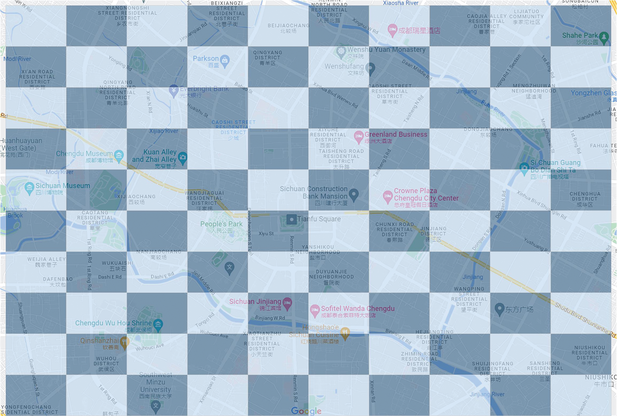
Figure 2: The figure shows the geographical location of the grids designed in this paper, with each grid covering approximately one to two blocks and having the same area

To ensure the spatial correlation of the data, we implemented grid division within a unified area, where each grid is positioned adjacent to its neighbouring grids. By considering each grid as a node and establishing connections between adjacent nodes, we derived an adjacency matrix that effectively captures the spatial characteristics of the data.

Subsequently, we geospatially matched the latitude and longitude coordinates of the floating car data with different grid regions. Initially, we determined the precise vehicle location based on the latitude and longitude data, followed by identifying the corresponding time range when the vehicle traversed through each region. Subsequently, we assigned a unique vehicle ID to each respective region. Notably, in cases where multiple instances of a vehicle’s data are recorded within the same region during an identical time period, redundant calculations are avoided.

By correlating the vehicle data with the urban area through the outlined steps, we conducted a statistical analysis of the vehicle IDs for all regions within a fixed time interval of 5 min. The statistical analysis was performed using Python, with pandas for data manipulation and aggregation, and scipy for statistical calculations. In this way, we obtained the traffic flow data for all regions every five minutes. Through the above processing, we finally received the Chengdu traffic flow dataset, which includes a 100 × 100 adjacency matrix representing the road network information and a 100 × 1296 feature matrix representing the traffic flow in different regions.

3.3.2 Road Monitoring Data for D4

To accurately depict the topological structure of the graph and derive the adjacency matrix for the dataset, this experiment established relevant nodes based on the geographical locations of road monitoring sensors. Given that these sensors are installed in bidirectional lanes at intersections, a total of eight nodes are designated per intersection to capture traffic data, with two nodes positioned on each side of the road. By employing this approach, a cumulative count of 24 nodes is established across three consecutive intersections. Subsequently, connections are made between corresponding nodes to account for vehicle movements involving left turns, straight-ahead directions, and right turns within each intersection. Finally, by linking the respective nodes in an upstream-to-downstream sequence for all three intersections involved, we obtained the resulting adjacency matrix for our dataset.

On the other hand, since the data recorded by the road monitoring sensors is traffic volume data, this experiment selected a fixed time interval of 5 min and processed the traffic data recorded by each node into traffic flow data. Through the aforementioned processing, a small-scale traffic flow dataset is finally obtained. The dataset includes a 24 × 24 adjacency matrix representing the positional correlation of nodes and a 24 × 8928 feature matrix representing traffic flow data for different nodes.

3.4 Capture of the Importance of Temporal Features

As a common and complex type of IoT time series data, traffic data has strong trends and patterns, including daily, weekly, and monthly trends. The regular fluctuation trends of traffic data are daily, weekly, and monthly. As shown below, we plot the processed flow and speed data as trends over time. Thus, capturing temporal correlations of traffic time series data essentially involves identifying the differences in the importance of different data features over a certain period for predicting future data. Since the collected data have different time dimensions, the daily trend is prioritised in this experiment. The trend plots of the dataset used in this paper are shown in Fig. 3.

Figure 3: (a) shows the traffic speed data from dataset D2 with a time interval of 15 min, and (b) shows the traffic flow data from dataset D4 with a time interval of 5 min. Both the flow and speed data have strong regularity, especially with similar daily trends. During peak hours in the morning and evening, the flow data increases significantly, and the average speed decreases noticeably

The data involved in traffic analysis typically exhibits a significant temporal dimension, necessitating the processing of extensive time-based information to capture the temporal correlations within traffic patterns. However, providing all this time-related data to the algorithm can lead to sluggish model iteration speed, demanding high computational resources such as computing power and memory, and even potential issues like overfitting, gradient vanishing, or explosion. Simultaneously, a specific type of IoT time series data primarily comprising traffic updates exhibits rapid fluctuations, necessitating the acceleration of prediction speed while ensuring accuracy. This entails enhancing algorithmic iteration speed and promptly delivering precise predictions to aid relevant authorities in guiding urban road traffic control and preemptively addressing potential issues concerning pertinent vehicles.

Due to the necessity of timely traffic data prediction, addressing the issue of reducing algorithm model iteration speed is crucial in traffic data processing and prediction. Numerous studies have demonstrated that the XGBoost algorithm effectively handles and predicts tabular data with rapid prediction speed and minimal computing power requirements. Additionally, its decision tree-based model ensures strong interpretability by numerically displaying feature importance. However, it lacks explicit spatial correlation representation. Hence, we establish three sets of lag time features to predict future conditions and determine which past time features yield optimal predictive performance.

In this study, we set up three different time capture strategies for four datasets to form a control experimental group, as shown in the following Fig. 4.

Figure 4: The figure illustrates the three-lag time feature construction schemes designed in this study. Scheme A represents the past ten-time units, Scheme B represents the ten-time units from the previous day, and Scheme C combines the two data sets

Fig. 4 shows the three temporal strategies adopted in this paper: Scheme A assembles the features of the past period, Scheme B assembles the time features of the previous day, and Scheme C combines Scheme A with Scheme B.

The three lagged time feature generation strategies designed in this paper are presented in Fig. 4. Each strategy is designed to capture different temporal aspects of traffic data to enhance predictive accuracy. Specifically, Scheme A incorporates the past 10-time units as lagged time features, which enables the model to consider recent trends in traffic data. Scheme B, on the other hand, uses the past 10-time units from the same time on the previous day, capturing daily periodicity and accounting for traffic patterns that may recur at similar times each day. Scheme C combines both Scheme A and Scheme B, allowing the model to leverage recent data trends alongside daily recurring patterns.

For each strategy, we employ the XGBoost algorithm to predict the current moment and assess feature importance, leveraging its decision tree-based approach for rapid calculation of feature relevance. By quantifying the importance of lagged features under each strategy, we aim to identify which temporal patterns whether recent trends, daily patterns, or a combination of both are most influential in predicting future traffic conditions. The feature importance results for these lagged features, evaluated across different datasets, are illustrated in Fig. 5.

Figure 5: The figure shows the importance of time features under three different lag strategies for the four datasets

Fig. 5 presents the importance scores for temporal features, obtained through the use of the XGBoost algorithm across four datasets. The results indicate that XGBoost is particularly adept at capturing data trends, as it assigns higher importance scores to features with a longer time span. This pattern is consistent across all datasets and is evident under three different lag strategies, highlighting the algorithm’s ability to recognize the significance of long-term temporal features in improving prediction accuracy.

3.5 Weighting and Dimensionality Reduction of Data and Neural Network Algorithm Prediction

We normalise each data group after obtaining the numerical values representing the importance of different lag time features. By normalising, we obtain the weight coefficients W corresponding to each lag feature. We then multiply the weight parameters by the corresponding feature values representing the time point. Finally, we sum all the data to obtain new time features, achieving the effect of dimensionality reduction.

For different strategies, we use different aggregation methods:

1. In Scheme A, we extract the features from the past two-time units separately and put the remaining values from 3 to 7-time units together for the aforementioned normalization and weighted sum operation.

2. In Scheme B, we extract the features from the past two-time units of the previous day separately and put the remaining values from 3 to 7-time units together for the aforementioned normalization and weighted sum operation.

3. In Scheme C, we extract the features from the past two time units and the current time unit of the previous day separately and put the remaining 17 time units’ values together for the aforementioned normalization and weighted sum operation.

After obtaining the corresponding parameters, we employ the LSTM-GR algorithm to construct our model. We decompose the intricate feature matrix into a spatial feature matrix and a time feature matrix through matrix factorisation. The spatial feature matrix is combined with the adjacency matrix for Laplacian transformation, while the time feature matrix is aggregated and reduced based on calculated parameters from the aforementioned schemes. Subsequently, we feed this reduced data into an LSTM algorithm to capture temporal correlations and ultimately output prediction results. Fig. 6 shows the full block diagram of the LSTM-GL_W experimental model, which illustrates the model structure and data flow.

Figure 6: The diagram is the full block diagram of LSTM-GL_W experimental model

Additionally, missing values may occur due to various collection issues in real-life traffic data, such as equipment malfunctions or signal interference. To validate the predictive performance of this approach in the presence of missing values in the dataset, the experiment sets 10% of random missing values. Subsequently, the dataset is partitioned into a training set and a testing set proportionally, and the three strategies mentioned above are employed for model training and prediction.

In this paper, the data without aggregation operation and the data with the aforementioned aggregation operation are put together to form a control group to investigate whether aggregating data will affect the prediction results.

3.6 Evaluation Metrics

Finally, through a comparative analysis of the predicted results against the actual observations, we derive experimental performance indicators and analyze their trends by plotting the data. Given that traffic data entails time series regression prediction, in this study, a selection of indicators commonly employed by researchers in regression prediction was adopted, including (1) Mean Absolute Error (MAE); (2) Mean Squared Error (MSE); (3) Root Mean Squared Error (RMSE); (4) R-squared (R2).

4  Results and Analysis

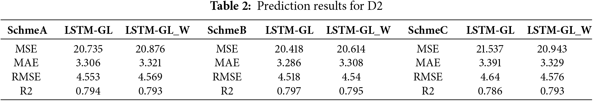
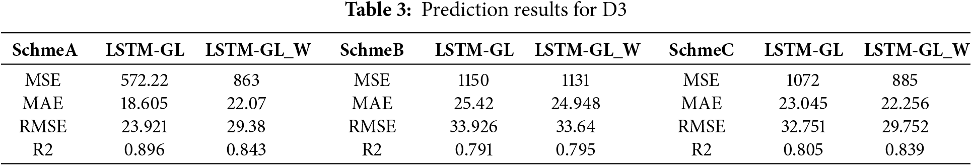
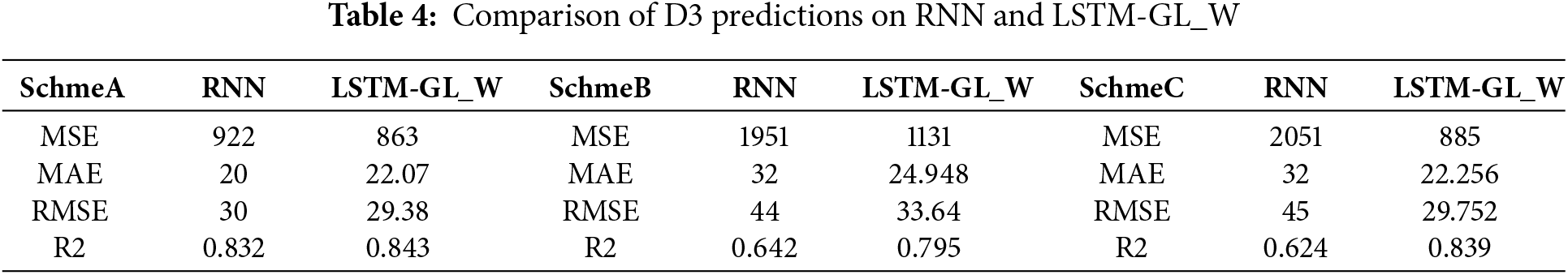
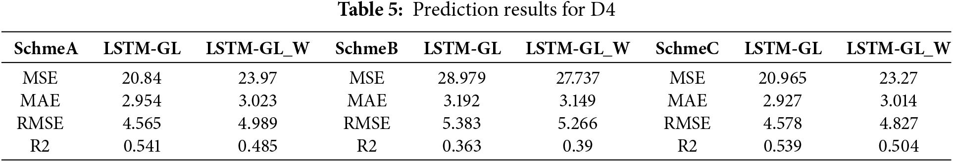
The relevant experimental results are shown in the table, where LSTM-GR represents the original neural network algorithm, and LSTM-GR_W represents the neural network algorithm with weight aggregation performed. The experimental results of D1 are shown in Table 1, the experimental results of D2 are shown in Table 2, the experimental results of D3 are shown in Table 3, the experimental results compared with RNN are shown in Table 4, and the experimental results of D4 are shown in Table 5.

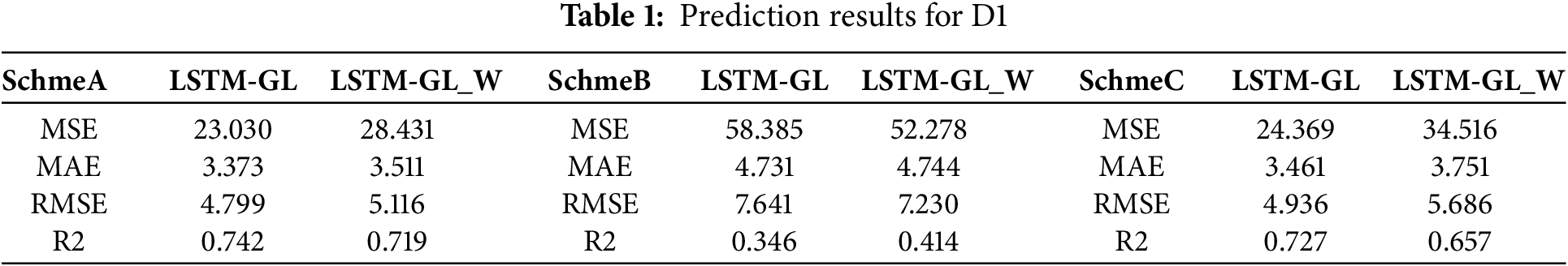
Regarding dataset D1, there is not much difference in the overall performance of the two algorithms. Under Scheme A, both algorithms perform well in prediction, with LSTM-GR showing better results with an R2 value of 0.742. However, under Scheme B, neither algorithm can predict future conditions well, with LSTM-GR_W showing slightly better results with an R2 value of 0.414. Under Scheme C, the LSTM-GR algorithm performs better than LSTM-GR_W with an R2 value of 0.727. Overall, the LSTM-GR algorithm shows better experimental results on dataset D1.

For dataset D2, both algorithms perform well under all three strategies. Under Scheme A, both algorithms show good performance in prediction, with the LSTM-GR algorithm performing slightly better with an R2 value of 0.794. Under Scheme B, LSTM-GR’s prediction results are still better than LSTM-GR_W, with an R2 value of 0.797. Under Scheme C, the LSTM-GR_W algorithm performs better than LSTM-GR with an R2 value of 0.793. Overall, both algorithms show good performance on dataset D2, and the performance difference between the two algorithms is not significant.

For dataset D3, the two algorithms have a certain performance gap. Under Scheme A, LSTM-GR’s prediction results are significantly better than LSTM-GR_W, with LSTM-GR having an R2 value of 0.896, which is 0.05 higher than LSTM-GR_W’s value. Under Scheme B, both algorithms show good performance, with LSTM-GR_W having an R2 value of 0.795, which is only 0.04 higher than LSTM-GR’s R2 value. Under Scheme C, LSTM-GR_W performs better than LSTM-GR, with an R2 value of 0.839. Although the two algorithms have different performances under different strategies, overall, LSTM-GR_W shows better experimental results on dataset D3.

For dataset D3, we compare the predictive performance of RNN and LSTM-GR_W across the three temporal feature schemes. The experimental results consistently demonstrate that LSTM-GR_W outperforms RNN in terms of prediction accuracy. Specifically, at shorter time lag intervals (fewer time units), RNN performs slightly worse than LSTM-GR_W, likely due to the inherent limitations of RNNs in capturing long-term dependencies within the data. As the time lag unit increases, the prediction results of RNN will be significantly worse than LSTM-GR_W. Overall, LSTM-GR_W performs better than RNN on this dataset.

Regarding dataset D4, there is not much difference in the overall performance of the two algorithms. Under Scheme A, both algorithms show average performance in prediction, with LSTM-GR showing better results with an R2 value of 0.541. Under Scheme B, neither algorithm can predict future conditions well, with LSTM-GR and LSTM-GR_W having R2 values of 0.363 and 0.39, respectively. Under Scheme C, the LSTM-GR algorithm performs better than LSTM-GR_W, with an R2 value of 0.539. Overall, both algorithms show average performance on dataset D4. The above experimental results indicate that both the LSTM-GR and LSTM-GR_W methods can provide reasonable predictions for the vast majority of datasets. Specifically, in Scheme A, the performance of LSTM-GR is better than that of LSTM-GR_W. However, in Scheme B, LSTM-GR_W tends to have better predictive performance than LSTM-GR. When facing Scheme C, LSTM-GR_W achieves better predictive results on datasets D2 and D3, while LSTM-GR performs better on datasets D1 and D4. At the same time, we compare with RNN. Both LSTM-GR and LSTM-GR_W show better ion prediction results than RNN. Overall, the performance of the two methods varies depending on the characteristics of the dataset. Scheme A performs better than Scheme C, and Scheme B performs worse. This indicates that the closer the input neural network algorithm is to the predicted time, the better the prediction effect.

Furthermore, we analysed that the D4 dataset covers the smallest range of the four datasets and has the fewest road nodes. This results in the neural network algorithm being unable to capture more node information during modeling, leading to poorer prediction results. However, as the range of the data expands and the number of nodes in the data increases, the neural network algorithm can effectively aggregate information from adjacent nodes to make more accurate predictions for future data.

Overall, the proposed LSTM-GR_W method shows good predictive performance when facing datasets with different characteristics, especially for data with longer time spans. The reason is that the proposed method effectively improves the capture of features for data with long time spans. At the same time, by reducing the number of neurons in the input layer, the method effectively reduces the complexity of the model and reduces the requirements of the model for hardware, such as computer memory and computing power.

5  Conclusion and Future Work

This study introduces a heuristic feature engineering method that extracts significant features from time series data using non-neural network algorithms. These features are aggregated to reduce model complexity and computational overhead, enabling the development of a more efficient approach for traffic prediction. By integrating these heuristic features with neural networks, the method offers flexibility for addressing diverse spatiotemporal data patterns. The effectiveness of the proposed method was evaluated through controlled experiments on four real-world datasets, including road sensor data and floating car data. The results demonstrate that the method not only improves prediction accuracy but also reduces computational demands, making it suitable for practical traffic applications. This approach provides a complementary perspective to existing neural network methods, emphasizing the importance of feature engineering in traffic data analysis.

Future work will focus on extending the method’s capabilities by comparing it with advanced models, such as Transformer and Informer, when larger datasets become available. Additionally, further exploration will aim to enhance the method’s adaptability to complex traffic conditions and investigate its integration with large-scale models.

Acknowledgement: The authors would like to express their gratitude for the valuable feedback and suggestions provided by all the anonymous reviewers and the editorial team.

Funding Statement: This work is supported by the Shandong Province Higher Education Young Innovative Talents Cultivation Programme Project: TJY2114, Jinan City-School Integration Development Strategy Project: JNSX2023015, and the Natural Science Foundation of Shandong Province: ZR2021M F074.

Author Contributions: The authors confirm contribution to the paper as follows: study conception and design: Bin Sun, Tao Shen, Yinuo Wang; data collection: Yinuo Wang; analysis and interpretation of results: Yinuo Wang, Lu Zhang, Renkang Geng; draft manuscript preparation: Yinuo Wang, Lu Zhang. All authors reviewed the results and approved the final version of the manuscript.

Availability of Data and Materials: The data that support the findings of this study are available from the corresponding author upon reasonable request.

Ethics Approval: Not applicable.

Conflicts of Interest: The authors declare no conflicts of interest to report regarding the present study.

References

1. Qin JY, Mei G, Lei X. Building the traffic flow network with taxi GPS trajectories and its application to identify urban congestion areas for traffic planning. Sustainability. 2021;13(1):266. [Google Scholar]

2. Sun B, Cheng W, Bai GH, Goswami P. Correcting and complementing freeway traffic accident data using mahalanobis distance based outlier detection. Technical Gazette. 2021;24:1597–607. [Google Scholar]

3. Sun B, Geng RK, Zhang L, Li S, Shen T, Ma LY. Securing 6G-enabled IoT/IoV networks by machine learning and data fusion. Eurasip J Wirel Comm. 2022;2022(1):113. doi:10.1186/s13638-022-02193-5. [Google Scholar] [CrossRef]

4. González D, Pérez J, Milanés V, Nashashibi F. A review of motion planning techniques for automated vehicles. IEEE Trans Intell Transp Syst. 2016;17(4):1135–45. doi:10.1109/TITS.2015.2498841. [Google Scholar] [CrossRef]

5. Fukuda S, Uchida H, Fujii H, Yamada T. Short-term prediction of traffic flow under incident conditions using graph convolutional recurrent neural network and traffic simulation. IEEE Trans Intell Transp Syst. 2020;14(8):936–46. doi:10.1049/iet-its.2019.0778. [Google Scholar] [CrossRef]

6. Badue C, Guidolini R, Carneiro RV, Azevedo P, Cardoso VB, Forechi A, et al. Self-driving cars: a survey. Expert Syst Appl. 2021;2021(165):113816. [Google Scholar]

7. Zhu FH, Lv LS, Chen YY, Wang X, Xiong G, Wang FY. Parallel transportation systems: toward IoT-enabled smart urban traffic control and management. IEEE Trans Intell Transp Syst. 2020 Oct;21(10):4063–71. doi:10.1109/TITS.6979. [Google Scholar] [CrossRef]

8. Hou ZX, Zhou YC, Du RH. Special issue on intelligent transportation systems, big data and intelligent technology. Transp Plan. 2016;39(8):747–50. doi:10.1080/03081060.2016.1231893. [Google Scholar] [CrossRef]

9. Cheng X, Duan DL, Yang LQ, Zheng NN. Societal intelligence for safer and smarter transportation. IEEE Internet Things J. 2021;8(11):9109–21. doi:10.1109/JIOT.2021.3057131. [Google Scholar] [CrossRef]

10. Cao DP, Li L, Marina C, Chen L, Xing Y, Zhuang WH. Special issue on internet of things for connected automated driving. IEEE Internet Things J. 2020;7(5):3678–80. doi:10.1109/JIoT.6488907. [Google Scholar] [CrossRef]

11. Wang XM, Zheng XH, Chen W, Wang FY. Visual human-computer interactions for intelligent vehicles and intelligent transportation systems: the state of the art and future directions. IEEE Trans Syst Man Cybern: Syst. 2020;51(1):253–65. [Google Scholar]

12. B Sun, W Cheng, P Goswami, and GH Bai, An overview of parameter and data strategies for k-nearest neighbours based short-term traffic prediction. In: Proceedings of the 2017 International Conference on E-Society, E-Education and E-Technology (ICSET 2017): 2017; New York, USA; ACM. pp. 68–74. [Google Scholar]

13. B Sun, C Wei, P Goswami, GH Bai, B Sun, W Cheng, et al. “Flow-aware WPT k-nearest neighbours regression for short-term traffic prediction. In: Proceedings of the 2017 IEEE Symposium on Computers and Communications (ISCC); 2017; Crete, Greece, Heraklion: IEEE. pp. 48–53. [Google Scholar]

14. Nguyen T, Nguyen G, Nguyen BM. EO-CNN: an enhanced CNN model trained by equilibrium optimization for traffic transportation prediction. Procedia Comput Sci. 2020;2020(176):800–9. [Google Scholar]

15. Zhao JD, Gao Y, Bai ZM, Wang H, Lu SH. Traffic speed prediction under non-recurrent congestion: based on LSTM method and BeiDou navigation satellite system data. IEEE Intell Transp Syst Mag. 2019;11(2):70–81. doi:10.1109/MITS.5117645. [Google Scholar] [CrossRef]

16. Meng XW, Fu H, Peng LQ, Liu GQ, Yu Y, Wang Z, et al. Short-term road traffic speed prediction model based on GPS positioning data. IEEE Trans Intell Transp Syst. 2020;23(3):2021–30. [Google Scholar]

17. Hu N, Zhang DF, Xie K, Liang W, Diao CY, Li K-C. Multi-range bidirectional mask graph convo-lution based GRU networks for traffic prediction. J Syst Archit. 2022;2022(133):102775. [Google Scholar]

18. Chen ZJ, Lu Z, Chen QS, Zhong HL, Zhang YS, Xue J, et al. Spatial-temporal short-term traffic flow prediction model based on dynamical-learning graph convolution mechanism. Inform Sci. 2022;2022(611):522–39. doi:10.1016/j.ins.2022.08.080. [Google Scholar] [CrossRef]

19. Xu XR, Zhang T, Xu CY, Cui Z, Yang J. Spatial-temporal tensor graph convolutional network for traffic speed prediction. IEEE Trans Intell Transp Syst. 2022;2022(1):92–3. doi:10.1109/TITS.2022.3215613. [Google Scholar] [CrossRef]

20. Zhang ZK, Li YD, Song HF, Dong HR. Multiple dynamic graph based traffic speed prediction method. Neurocomputing. 2021;2021(461):109–17. doi:10.1016/j.neucom.2021.07.052. [Google Scholar] [CrossRef]

21. Hu XJ, Liu T, Hao XT, Lin CX. Attention-based Conv-LSTM and Bi-LSTM networks for large-scale traffic speed prediction. J Supercomput. 2022;78(10):12686–709. doi:10.1007/s11227-022-04386-7. [Google Scholar] [CrossRef]

22. Su ZY, Liu T, Hao XT, Hu XJ. Spatial-temporal graph convolutional networks for traffic flow prediction considering multiple traffic parameters. J Supercomput. 2023;79(16):18293–312. doi:10.1007/s11227-023-05383-0. [Google Scholar] [CrossRef]

23. Fanhui K, Li J, Jiang B, Song HB. Short-term traffic flow prediction in smart multimedia system for Internet of Vehicles based on deep belief network. Future Gener Comput. 2019;93(8):460–72. doi:10.1016/j.future.2018.10.052. [Google Scholar] [CrossRef]

24. Abadi A, Rajabioun T, Ioannou PA. Traffic flow prediction for road transportation networks with limited traffic data. IEEE Trans Intell Transp Syst. 2015;16(2):653–62. [Google Scholar]

25. Hengl T, Nussbaum M, Wright MN, Heuvelink GBM, Gräler B. Random forest as a generic framework for predictive modeling of spatial and spatio-temporal variables. PeerJ. 2018;6(8):5518. doi:10.7717/peerj.5518. [Google Scholar] [PubMed] [CrossRef]

26. Niu WN, Li T, Zhang XS, Hu T, Jiang TY, Wu H. Using XGBoost to discover infected hosts based on HTTP traffic. Secur Commun Networks. 2019;2019(1):2–16. doi:10.1155/2019/2182615. [Google Scholar] [CrossRef]

27. Zhang XJ, Zhang QR. Short-term traffic flow prediction based on LSTM-XGBoost combination mode. Comp Model Eng Sci. 2020;125(1):95–109. doi:10.32604/cmes.2020.011013. [Google Scholar] [CrossRef]

28. Reiter JP. Using CART to generate partially synthetic public use microdata. J Off Stat. 2005;21:441–62. [Google Scholar]

29. Gu JX, Wang ZH, Kuen J, Ma LY, Shahroudy A, Shuai B, et al. Recent advances in convolutional neural networks. Pattern Recognit. 2018;77:354–77. doi:10.1016/j.patcog.2017.10.013. [Google Scholar] [CrossRef]

30. Medsker LR, Jain LC. Recurrent neural networks. Des Appl. 2001;5:64–7. [Google Scholar]

31. Zhou J, Cui GQ, Hu SD, Zhang ZY, Yang C, Liu Z, et al. Graph neural networks: a review of methods and applications. AI Open. 2020;1:57–81. doi:10.1016/j.aiopen.2021.01.001. [Google Scholar] [CrossRef]

32. Shen YF, Wu YJ, Zhang Y, Shan CH, Zhang J, Letaief KB, et al. How powerful is graph convolution for recommendation? In: CIKM ’21: Proceedings of the 30th ACM International Conference on Information & Knowledge Management; 2021. p. 1619–29. doi:10.1145/3459637.3482264. [Google Scholar] [CrossRef]

33. Veličković P, Cucurull G, Casanova A, Romero A, Liòet P, Bengio Y. Graph attention networks. arXiv:1710.10903. 2017. [Google Scholar]

34. Kipf TN, Welling M. Variational graph auto-encoders. arXiv:1611.07308. 2016. [Google Scholar]

35. Jin WG, Yang K, Barzilay R, Jaakkola T. Learning multimodal graph-to-graph translation for molecular optimization. arXiv:1812.01070. 2018. [Google Scholar]

36. Sahili ZA, Awad M. Spatio-temporal graph neural networks: a survey. arXiv:2301.10569. 2023. [Google Scholar]

37. Jiang HW, Qin FW, Cao J, Peng Y, Shao YL. Recurrent neural network from adder’s perspective: carry-lookahead RNN. Neural Netw. 2021;144:297–306. doi:10.1016/j.neunet.2021.08.032. [Google Scholar] [PubMed] [CrossRef]

38. Ma CX, Dai GW, Zhou JB. Short-term traffic flow prediction for urban road sections based on time series analysis and LSTM_BILSTM method. IEEE Trans Intell Transp Syst. Jun 2022;23(6):5615–24. doi:10.1109/TITS.2021.3055258. [Google Scholar] [CrossRef]

39. Wang Y, Zhang Y, Piao XL, Liu H, Zhang K. Traffic data reconstruction via adaptive spatial-temporal correlations. IEEE Trans Intell Transp Syst. 2019;20(4):1531–43. doi:10.1109/TITS.6979. [Google Scholar] [CrossRef]

40. Maretic HP, Frossard P. Graph laplacian mixture model. IEEE Trans Signal Inf Process Over Netw. 2020;6:261–70. doi:10.1109/TSIPN.6884276. [Google Scholar] [CrossRef]

41. Yang JM, Peng ZR, Lin L. Real-time spatiotemporal prediction and imputation of traffic status based on LSTM and Graph Laplacian regularized matrix factorization. Transp Res Part C: Emerg Technol. 2021;129:103–228. [Google Scholar]