Delocalized Nonlinear Vibrational Modes in Bcc Lattice for Testing and Improving Interatomic Potentials

1  Introduction

Molecular dynamics (MD) method is a powerful tool for the analysis of crystal lattice defects, phase transitions, and mechanical properties of solids. The success of the method is related to advances in the development of accurate interatomic potentials, as reflected in the following reviews [1–4], including reactive potentials [5] and those for modeling ceramics, glass, and electrolytes [6]. Recently, machine learning techniques have been used to improve the accuracy of interatomic potentials, typically by training on first-principles results for random atomic configurations [7,8].

Since in this work the bcc lattice is analyzed, it is important to describe the works devoted to metals with this lattice symmetry. MD method has been successfully used for modeling bcc metals, in particular, the dislocations and Peierls barrier [9–13], diffusion properties [14–17], cleavage [13,18], properties of bcc iron [19], vanadium [20], tungsten [21–23], tantalum [24], zirconium and uranium [25], phase transitions in iron [26], scandium [27], lithium [28] and magnesium [29], crack propagation [30], mechanical behavior of nanowires [31], vacancy clusters [32], structure of twin boundary [33], radiation damage [34,35], surface energy [36], atomistic fracture [37], grain boundary structure and mobility [38,39], melting [40], and magnetic properties [41–43]. The accuracy of interatomic potentials has been analyzed for carbon polymorphs and metal-graphene composites [44–47].

Work on the further improvement of interatomic potentials for metals continues [48–51], with one of the main problems being the finding of the data set for potential training. In this paper, the properties of the exact solutions of the equations of atomic motion in the bcc lattice are analyzed and offered for testing and improving the interatomic potentials, as described in the works [52,53].

Crystal lattices admit exact dynamical solutions in the form of delocalized nonlinear vibrational modes (DNVMs). Such solutions can be derived considering only the space symmetry group of the lattice [54–57] and thus exist for any type of interatomic interactions even at large amplitudes.

Let us describe some important literature where DNVMs have been constructed and analyzed for different lattices. An n-component DNVM represents a vibrational mode with n degrees of freedom; one-component DNVMs are actually the Rosenberg modes [58]. DNVMs are the short wavelength vibrational modes, they can have wave vectors at the boundary of the first Brillouin zone or inside it. In this study, only the former are analyzed. One- and two-component DNVMs of triangular lattice have been studied in [59] and one-component DNVMs of square lattice in [60]. More recently, DNVMs in three-dimensional lattices have been studied, including the simple cubic [61], fcc [62], and bcc [63] lattices. In most cases, DNVMs are studied in lattices with nearest neighbor interactions, or considering the first and second neighbors, e.g., for the square lattice, since this lattice is unstable if the second neighbor bonds are not involved. There is a close relationship between DNVMs in two-dimensional [64–66] and three-dimensional [67–70] lattices and spatially localized nonlinear vibrational modes called discrete breathers or intrinsic localized modes.

DNVMs can be used efficiently to check the quality of interatomic potentials [52,71], and to solve this problem for metals, long-range interactions should be taken into account. This follows from the nature of the metallic bonds, since the outermost electron shell of the metal atoms overlaps with a large number of neighboring atoms.

An important feature of this work is that the interactions are considered up to the fourth neighbor, and it is relevant to describe some works where the effect of long-range interactions has been studied. The long-range interactions have been included in many papers analyzing nonlinear lattice dynamics. In particular, long-range interactions have been taken into account in the study of discrete breathers in DNA [72–76], in chains with Coulomb forces [77,78] and dispersive interactions [79]. The effect of long-range interactions on heat transport in chains has been addressed in the works [80,81]. The mobility of discrete breathers increases in the lattices with long-range interactions [82,83].

Phonon dispersion curves are very informative in characterizing crystal lattice dynamics and many studies have been done for bcc metals, let us mention some of them. The dispersion curves are often used to test and fit interatomic potentials, see for example the work [84,85] dealing with the bcc alkali metals Li, Na, K, Rb, and Cs as well as the work [86] devoted to the bcc transition metals Cr, Fe, Mo, Nb, Ta, V, and W. Elastic anisotropy and temperature-dependent phonon dispersion for bcc Fe and W have been studied by molecular dynamics simulations [87]. The first-principles study of the phonon spectra for highly compressed Sb has shown that the stability of the bcc structure increases with pressure [88]. The choice of interatomic potentials to model the metastable bcc polymorph of Mg, taking into account the phonon dispersion curves and other properties, has been discussed in [89]. Molecular dynamics simulations with machine learning potential have been performed for the high-temperature bcc phase of zirconium [90]. The ab initio study of the dispersion curves of bcc transition metals (vanadium and niobium) has demonstrated the importance of considering the supercell of sufficiently large size [91].

In view of the aforementioned interest in the phonon dispersion of the bcc lattice in metals, here we derive analytically the phonon dispersion relation for the bcc lattice taking into account the interactions up to the fourth neighbor. Then the 34 DNVMs are introduced, their wavevectors are given, and the frequency in the small amplitude limit is calculated analytically. The frequency response of the DNVMs is calculated numerically, assuming that the atoms interact via the β-Fermi-Past-Ulam-Tsingu (FPUT) potential.

The main goal of this work is to describe the properties of the DNVMs, which are the family of exact large-amplitude vibrational solutions for the bcc lattice. These solutions can be used to test the accuracy of the interatomic potentials of crystals with this lattice. The accuracy of the potentials can be checked by comparing the frequency response of DNVMs calculated with this or that interatomic potential with that calculated using the more accurate ab initio approach. The choice of the β-FPUT potential is not essential in our work, since the DNVMs exist as exact solutions for any kind of interatomic interactions, since they are found considering only the symmetry of the lattice. Importantly for the problem of testing and fitting interatomic potentials, the fraction of potential energy stored by bonds of different lengths is calculated for each DNVM in the small-amplitude and large-amplitude regimes. Some examples of the derivation of the frequency response of DNVMs using the cubic approximation are presented.

The bcc lattice and the computational model are described in Section 2, then the DNVMs with the wavevectors at the boundary of the first Brillouin zone are presented in Section 3, the phonon dispersion relation for the lattice is derived and analyzed in Section 4, the distribution of the potential energy over the bonds of different length is discussed in Section 5, the frequency response of some DNVMs in cubic approximation is derived in Section 6. The results are discussed and summarized in Section 7.

2  Body-Centered Cubic Lattice

A three-dimensional body-centered cubic (bcc) lattice with up to the fourth nearest neighbor interactions is analyzed, see Fig. 1. The lattice parameter is h; the vectors specifying the primitive translational cell of the lattice are e1=(h,0,0), e2=(0,h,0), and e3=(h/2,h/2,h/2). Then the radius vectors of the lattice points are

ξi,j,k=ie1+je2+ke3,(1)

where i, j, and k are integers.

Figure 1: Body-centered cubic lattice with lattice parameter h. The primitive translational cell of the lattice is specified by the vectors e1, e2 and e3 (shown in magenta). The radius vectors of the first, second, third and fourth neighbors of the particle at the origin are depicted in red

The displacement of the particle i,j,k from its equilibrium position is defined by the vector δi,j,k=(ui,j,k,vi,j,k,wi,j,k). The position of this particle at time t is defined by the radius vector ri,j,k(t)=ξi,j,k+δi,j,k(t).

Each particle interacts with four nearest neighbors via the β-Fermi-Past-Ulam-Tsingou (β-FPUT) potential

φl(r)=cl2(r−al)2+βl4(r−al)4,l=1,…,4,(2)

where r is the distance between two particles; the distances between the first four neighbors are a1=3h/2, a2=h, a3=2h, and a4=11h/2; cl and βl define the linear and nonlinear stiffness of the l-th nearest bond, respectively. Using the lattice parameter as the length unit, h=1 is set. By choosing the unit of energy, c1=1 is set. In crystals the bond stiffness decreases with its length; therefore, it is assumed:

c1=1>c2>c3>c4>0.(3)

In the simulations, the following values of the linear stiffness parameters are assumed to satisfy Eq. (3):

c1=1,c2=0.9,c3=0.8,c4=0.7.(4)

In crystals, anharmonicity plays a prominent role when the displacements of the atoms are about 10% of the interparticle distance. With this in mind, the following values are used for the nonlinear stiffness coefficients:

β1=10.0,β2=9.0,β3=8.0,β4=7.0.(5)

The particle mass is m=1, which can always be obtained by choosing a time unit.

There are I×J×K particles in the computational cell. To mitigate the impact of free surfaces, periodic boundary conditions are implemented ri,j,k=ri+I,j,k=ri,j+J,k=ri,j,k+K.

The Hamiltonian of the considered lattice is the sum of the kinetic energy of the particles and the potential energies of the bonds up to the fourth neighbors:

H=K+P1+P2+P3+P4=∑i=1I∑j=1J∑k=1Km2|r˙i,j,k|2+12∑i=1I∑j=1J∑k=1K[∑s=18φ1(|Ri,j,k,s|)+∑s=914φ2(|Ri,j,k,s|)+∑s=1526φ3(|Ri,j,k,s|)+∑s=2750φ4(|Ri,j,k,s|)],(6)

where derivative with respect to time is denoted by the overdot and the vectors Ri,j,k,s connecting the atom i,j,k with its neighbors are given by Eqs. (A1)–(A4) in Appendix A.

The following equations of motion can be derived from the Hamiltonian Eq. (6):

mu¨i,j,k=∑s=18D1Ri,j,k,s,x+∑s=914D2Ri,j,k,s,x+∑s=1526D3Ri,j,k,s,x+∑s=2750D4Ri,j,k,s,x,mv¨i,j,k=∑s=18D1Ri,j,k,s,y+∑s=914D2Ri,j,k,s,y+∑s=1526D3Ri,j,k,s,y+∑s=2750D4Ri,j,k,s,y,mw¨i,j,k=∑s=18D1Ri,j,k,s,z+∑s=914D2Ri,j,k,s,z+∑s=1526D3Ri,j,k,s,z+∑s=2750D4Ri,j,k,s,z,(7)

where

Dl=φl′(|Ri,j,k,s|)|Ri,j,k,s|,l=1,…,4.(8)

The size of the computational cell to study the zone-boundary DNVMs is equal to 2h×2h×2h. The coordinates of 16 atoms in the cell are given in Fig. 2.

Figure 2: The coordinates of the atoms within the cubic translational cell, which has dimensions of 2h×2h×2h. The cell includes 16 atoms

The symplectic Störmer method of sixth order [92] is employed in this study to solve numerically the equations of motion Eq. (7). It is sufficient to take the integration step of 0.001 time units, as found in the test numerical runs.

3  Zone-Boundary DNVMs of bcc Lattice

A class of lattice symmetry dictated exact solutions to the nonlinear equations of motion of the bcc lattice is presented here. In the pioneering works such solutions were called bushes of nonlinear normal modes (BNNMs) [93], but in the context of crystal lattices the term DNVMs is often used.

The zone-boundary DNVMs are excited by giving the particles initial displacements according to certain patterns shown in Figs. 3 through 9. The initial velocities of the particles are zero. Trajectories of vibrating particles are shown in black. For particles represented by empty circles, the w-component of the initial displacement is zero, and it is positive (negative) if the particle is marked with a dot (cross).

Figure 3: Three DNVMs of group G1. The coordinates of the lattice positions of the atoms are presented in Fig. 2

All DNVMs are single degree of freedom vibrational modes. This means that the length of the initial displacement vector is either zero or A, the latter being the DNVM amplitude. The particles with zero initial displacement remain at rest while other particles oscillate.

All DNVMs are divided into seven groups, designated G1 through G7. Numerically determined frequency responses for the DNVMs are shown in Fig. 10 (groups G1, G2, and G3), Fig. 11 (groups G4 and G5), and Fig. 12 (groups G6 and G7) for the model parameters given by Eqs. (4) and (5). As can be seen in Figs. 10–12, DNVMs belonging to the same group have the same vibration frequency in the small amplitude limit. For large amplitudes, the frequency of modes in the same group is different. Different DNVMs of the same group have the same small amplitude vibration frequencies because more complex DNVMs are superpositions of a simple DNVM. For example, DNVM G1b in Fig. 3 is a superposition of DNVM G1a and its rotation by π/2 around the z axis; DNVM G1c is the sum of G1b and G1a rotated by π/2 around the y axis. All of the DNVMs demonstrate a hard-type anharmonicity, meaning that their vibration frequency increases with amplitude.

4  Phonon Dispersion Relation

To obtain the analytical expressions for the DNVM frequencies in the small amplitude limit, the phonon dispersion relation is derived from the linearized equations of motion. Such equations of motion can be derived from Eq. (7) under the assumption |δi,j,k|≪h and are listed in Appendix A, Eqs. (A6)–(A8). The solution of these equations is given in the standard form

ui,j,k=Uexp⁡[i(qi+sj+pk−ωt)],vi,j,k=Vexp⁡[i(qi+sj+pk−ωt)],wi,j,k=Wexp⁡[i(qi+sj+pk−ωt)],(9)

where (U,V,W) is the eigenvector, (q,s,p) is the wavevector, and i denotes the imaginary unit. By substituting Eq. (9) into Eqs. (A6)–(A8), one obtains the following set of linear algebraic equations:

(mω2+P1)U+ZV+SW=0,ZU+(mω2+P2)V+QW=0,SU+QV+(mω2+P3)W=0,(10)

P1=−γ1−γ2−γ3−γ4−ξ1−ϕ1−ϕ2−ϕ5−ϕ6−9δ1−9δ2−9δ3−9δ4−δ5−δ6−δ7−δ8−δ9−δ10−δ11−δ12,P2=−γ1−γ2−γ3−γ4−ξ2−ϕ1−ϕ2−ϕ3−ϕ4−δ1−δ2−δ3−δ4−δ5−δ6−δ7−δ8−9δ9−9δ10−9δ11−9δ12,P3=−γ1−γ2−γ3−γ4−ξ3−ϕ3−ϕ4−ϕ5−ϕ6−δ1−δ2−δ3−δ4−9δ5−9δ6−9δ7−9δ8−δ9−δ10−δ11−δ12,Z=−γ1+γ2−γ3+γ4−ϕ1+ϕ2−3δ1+3δ2+3δ3−3δ4−δ5+δ6+δ7−δ8−3δ9+3δ10−3δ11+3δ12,S=−γ1+γ2+γ3−γ4−ϕ5+ϕ6−3δ1−3δ2+3δ3+3δ4−3δ5+3δ6−3δ7+3δ8−δ9+δ10+δ11−δ12,Q=−γ1−γ2+γ3+γ4−ϕ3+ϕ4−δ1+δ2−δ3+δ4−3δ5−3δ6+3δ7+3δ8−3δ9−3δ10+3δ11+3δ12,(11)

γ1=4c13sin2⁡p2,γ2=4c13sin2⁡q−p2,γ3=4c13sin2⁡q+s−p2,γ4=4c13sin2⁡s−p2,ξ1=4c2sin2⁡q2,ξ2=4c2sin2⁡s2,ξ3=4c2sin2⁡q+s−2p2,ϕ1=4c32sin2⁡q+s2,ϕ2=4c32sin2⁡q−s2,ϕ3=4c32sin2⁡q−2p2,ϕ4=4c32sin2⁡q+2s−2p2,ϕ5=4c32sin2⁡s−2p2,ϕ6=4c32sin2⁡2q+s−2p2,δ1=4c411sin2⁡q+p2,δ2=4c411sin2⁡q−s+p2,δ3=4c411sin2⁡2q−p2,δ4=4c411sin2⁡2q+s−p2,δ5=4c411sin2⁡q+s−3p2,δ6=4c411sin2⁡2q+s−3p2,δ7=4c411sin2⁡q+2s−3p2,δ8=4c411sin2⁡2q+2s−3p2,δ9=4c411sin2⁡s+p2,δ10=4c411sin2⁡−q+s+p2,δ11=4c411sin2⁡q+2s−p2,δ12=4c411sin2⁡2s−p2.(12)

From the condition of zero determinant, one finds the following cubic in ω2 equation:

m3ω6+(P1+P2+P3)m2ω4+(P1P2+P2P3+P1P3−Q2−S2−Z2)mω2+P1P2P3−Q2P1−S2P2−Z2P3+2QSZ=0.(13)

The cubic in ω2 equation, Eq. (13), has three roots, corresponding to the dispersion relations for the three types of phonon modes of the bcc lattice.

The dispersion relations along the high symmetry lines of the first Brillouin zone are plotted in Fig. 13. The linear stiffness coefficients here and in the following are given by Eq. (4). Frequencies of different groups of DNVMs in the small-amplitude limit are indicated in blue. The frequencies and the wavevectors of DNVMs are listed in Table 1.

Substituting the wavevectors (q,s,p) given in Table 1 into Eq. (12), one finds the relations Eq. (11), which specify the set of equations Eq. (10) for finding the analytical expressions for the phonon frequencies. The results are as follows:

The group G1 DNVMs in the small-amplitude limit have frequency

mω2=83c1+4c2+8c3+8c4.(14)

Similar result for the group G2 DNVMs is

mω2=163c1+16c4.(15)

For the group G3 DNVMs, one has

mω2=163c1+4c2+4c3+4811c4.(16)

For the group G4 DNVMs, the frequency of small-amplitude vibrations is

mω2=4c2+4c3+12811c4.(17)

The group G5 DNVMs in the small-amplitude limit have frequency

mω2=83c1+8c3+8c4,(18)

For the group G6 DNVMs, the result is

mω2=83c1+4c2+8c4.(19)

Finally, the group G7 DNVMs in the small-amplitude limit have frequency

mω2=83c1+4c3+8c4.(20)

It is important to note that only DNVMs from groups G1 and G3 exhibit frequencies that are contingent on all four stiffnesses, cl, l=1,…,4. The frequencies of group G2 DNVMs depend only on c1 and c4; the frequencies of group G4 DNVMs do not depend on c1, the frequencies of groups G5 and G7 DNVMs do not depend on c2, and the frequencies of group G6 DNVMs do not depend on c3.

5  Energy of Different Bonds

As outlined in Section 4, the small-amplitude vibration frequencies of certain groups of DNVMs depend not on all stiffness coefficients. To further investigate the different contributions of different bonds to the DNVM dynamics, the fraction of the total potential energy stored by the bonds of different lengths is calculated for all DNVMs. This is done for the two values of the displacement of the atoms from the lattice positions, A=10−4 and A=0.3; the results are presented in Tables 2 and 3, respectively.

As can be seen from Table 2, different bonds contribute differently to the small-amplitude vibrations of DNVMs of different groups, and this contribution correlates with the coefficients in the analytical expressions for DNVM frequencies, Eq. (14) through Eq. (20). The result for the DNVMs belonging to the same group is identical, if the vibration amplitude is small. For the large amplitude vibrations, as can be seen from Table 3, the result is different for different DNVMs of the same group; this is the effect of anharmonicity. Nevertheless, the second- and third-neighbor bonds are not deformed when the G2 group DNVMs are excited even at large amplitudes. The same can be said about the third-neighbor bonds when G6 group DNVMs are excited.

6  Analytical Results for DNVMs

DNVM is an oscillatory mode with one degree of freedom. The displacement of any moving particle from its equilibrium position, a(t), is taken as the time-dependent variable. Below, for some DNVMs, a Hamiltonian H(a˙,a) is derived, keeping the quartic terms in a, then the cubic equation of motion is obtained and an approximate relationship between frequency and amplitude is derived and compared with the numerical results. The DNVMs chosen for the analysis will help to illustrate some important features of this class of exact dynamical solutions.

6.1 DNVM G1a

Considering a translational cell of the considered DNVM, the kinetic and potential energies per atom are calculated taking into account the displacement pattern of the particles, see Fig. 3, when the distance of the moving particles from the lattice positions is equal to a. The potential energy is then expanded in Taylor series up to the fourth order terms. The result is the following Hamiltonian:

H=ma˙24+(2c13+c2+2c3+2c4)a2+(−8c127h2−3c32h2+104c41331h2+β19+2β2+2β3+83β4121)a4.(21)

Note that in DNVM G1a only half of the atoms are vibrating and the other half are at rest, so the effective mass is equal to m/2. From the Hamiltonian Eq. (21) the following cubic equation of motion is derived:

ma¨=−4(2c13+c2+2c3+2c4)a−8(−8c127h2−3c32h2+104c41331h2+β19+2β2+2β3+83β4121)a3.(22)

An approximate solution to Eq. (22) includes the third harmonic correction to the main harmonic, a(t)=Asin⁡(ωt)+A1sin⁡(3ωt), where A1≪A. Substitution of this solution into Eq. (22) yields the following frequency response for DNVM G1a:

ω2≈4m(2c13+c2+2c3+2c4)+6m(−8c127h2−3c32h2+104c41331h2+β19+2β2+2β3+83β4121)A2.(23)

6.2 DNVM G2b

Similarly, the Hamiltonian for DNVM G2b is

H=ma˙22+8(c13+c4)a2+16(−8c127h2+104c41331h2+β19+83β4121)a4.(24)

Therefore, the cubic equation of motion is

ma¨=−16(c13+c4)a−64(−8c127h2+104c41331h2+β19+83β4121)a3,(25)

and the frequency response for DNVM G2b is

ω2≈16m(c13+c4)+48m(−8c127h2+104c41331h2+β19+83β4121)A2.(26)

6.3 DNVM G2c

Analogously, the Hamiltonian for DNVM G2c has the form

H=ma˙22+8(c13+c4)a2+8(2c127h2−73c41331h2+4β19+140β4121)a4.(27)

The cubic equation of motion is

ma¨=−16(c13+c4)a−32(2c127h2−73c41331h2+4β19+140β4121)a3.(28)

The frequency response for DNVM G2c is

ω2≈16m(c13+c4)+24m(2c127h2−73c41331h2+4β19+140β4121)A2.(29)

6.4 DNVM G6b

Finally, the Hamiltonian for DNVM G6b is

H=ma˙24+(2c13+c2+2c4)a2+(−8c127h2+2c2h2+104c41331h2+β19+2β2+83β4121)a4.(30)

The equation of motion for DNVM G6b is

ma¨=−4(2c13+c2+2c4)a−8(−8c127h2+2c2h2+104c41331h2+β19+2β2+83β4121)a3.(31)

The frequency response for DNVM G6b is

ω2≈4m(2c13+c2+2c4)+6m(−8c127h2+2c2h2+104c41331h2+β19+2β2+83β4121)A2.(32)

6.5 Discussion of the Analytical Results

A comparison of the analytical expressions for the frequency response with the numerical results is given for the four DNVMs analyzed in Fig. 14. The result is quite good, as the difference between the cubic approximation and the numerical result is only noticeable for A>0.1.

As can be seen from Fig. 14, the vibrational frequency of DNVMs depends on the amplitude, and there are two reasons for this. The first is the effect of the anharmonicity of the interparticle interactions, βl≠0, in Eq. (2). The second is the so-called geometric nonlinearity. The contributions of these two sources of frequency variation can be seen from the analytical expressions Eqs. (23), (26), (29), and (32). It can be seen that in the limit A→0 the DNVM frequency is a constant depending on the particle mass m and the linear stiffness coefficients cl. With increasing A different scenarios are possible and we discuss them for the frequency of the DNVM G1a by analyzing Eq. (23). If the term before A2 is positive (negative), the frequency will increase (decrease) with increasing A. In the case of soft-type anharmonicity, when βl<0, and for not very large c4, the frequency ω will decrease with increasing amplitude A. Interestingly, even for βl=0, l=1,…,4, i.e., for linear elastic bonds, the frequency can either increase or decrease with amplitude due to geometric nonlinearity. The frequency increases when (104/1331)c4>(8/27)c1+(3/2)c3 and decreases in the opposite case.

The deviation of the analytical results from the numerically found frequency response observed in Fig. 14 is due to the fact that in the Hamiltonians Eqs. (21), (24), (27), and (30) the terms higher than quartic are omitted and therefore the analytical results are approximate and their accuracy is high only for not very large vibration amplitudes.

Note that for each DNVM, the harmonic part of the frequency response matches the result of the linear analysis. This can be seen by comparing the harmonic part of Eq. (23) with Eq. (14), the harmonic parts of Eqs. (26) and (29) with Eq. (15), as well as the harmonic part of Eq. (32) with Eq. (19). It can also be noticed that the frequency responses of DNVMs belonging to the same group coincide in the small amplitude limit, but deviate as the vibration amplitude increases, compare Eqs. (26) and (29) obtained for the two DNVMs of group G2.

Notably, the frequency responses of the G2 group DNVMs do not depend on the parameters of the second and third neighbor bonds even for large vibration amplitudes. Similarly, the frequency responses of the G6 group DNVMs do not depend on c3 and β3 even for large vibration amplitudes. This is consistent with the numerical data presented in Table 3.

7  Conclusions

In short, for the first time, the linear and nonlinear dynamics of the bcc lattice have been analyzed considering long-range interactions, which is important for metals. The phonon dispersion relation was derived analytically. The properties of the exact nonlinear vibrational solutions, called DNVMs, have been analyzed analytically and numerically and offered as a dataset for training the machine learning interatomic potentials for bcc metals.

In more detail, the exact solutions of the equations of motion of the β-FPUT lattice in the form of DNVMs have been analyzed considering long-range interactions. The patterns of initial displacements of the atoms for the 34 DNVMs studied are shown in Figs. 3 to 9. Atoms with such initial displacements and zero initial velocities will oscillate, maintaining the pattern regardless of the interatomic potential used and for any amplitude A (for a large A, the DNVMs are modulationally unstable). However, the frequency response of a DNVM depends on the interatomic potential, and thus it can be used to test and develop interatomic potentials.

Figure 4: Three DNVMs of group G2

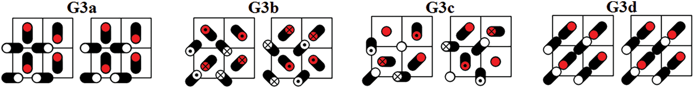
Figure 5: Four DNVMs of group G3

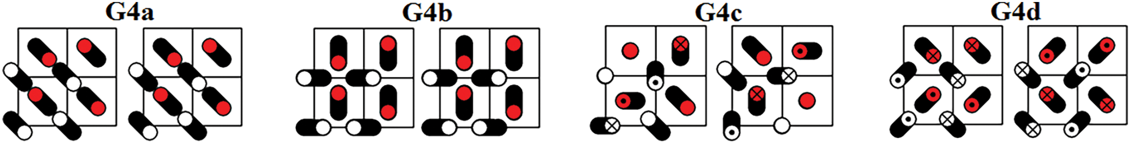
Figure 6: Four DNVMs of group G4

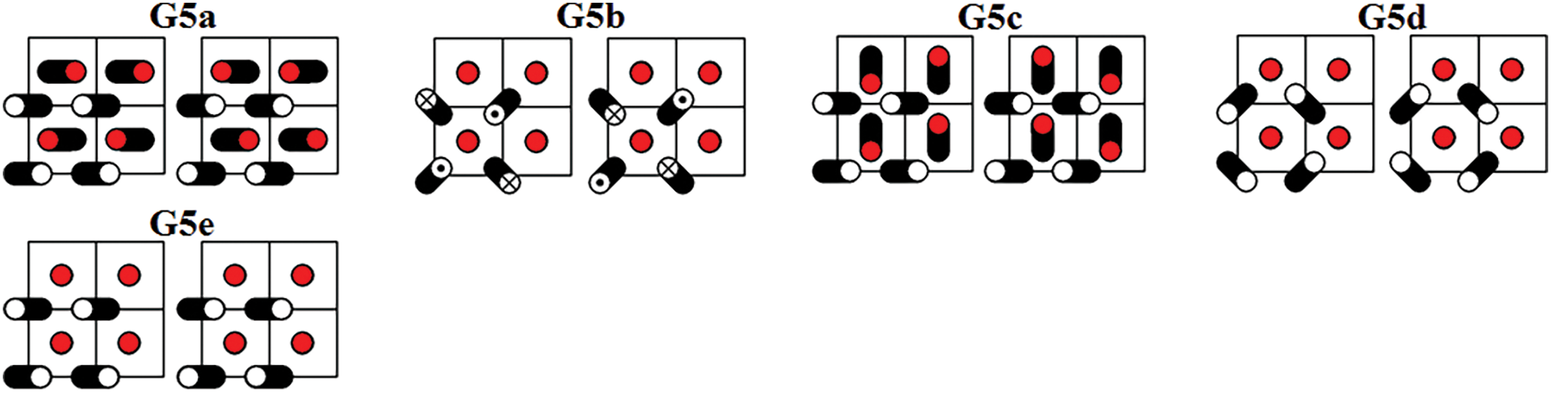
Figure 7: Five DNVMs of group G5

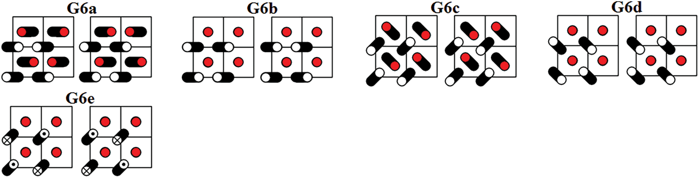
Figure 8: Five DNVMs of group G6

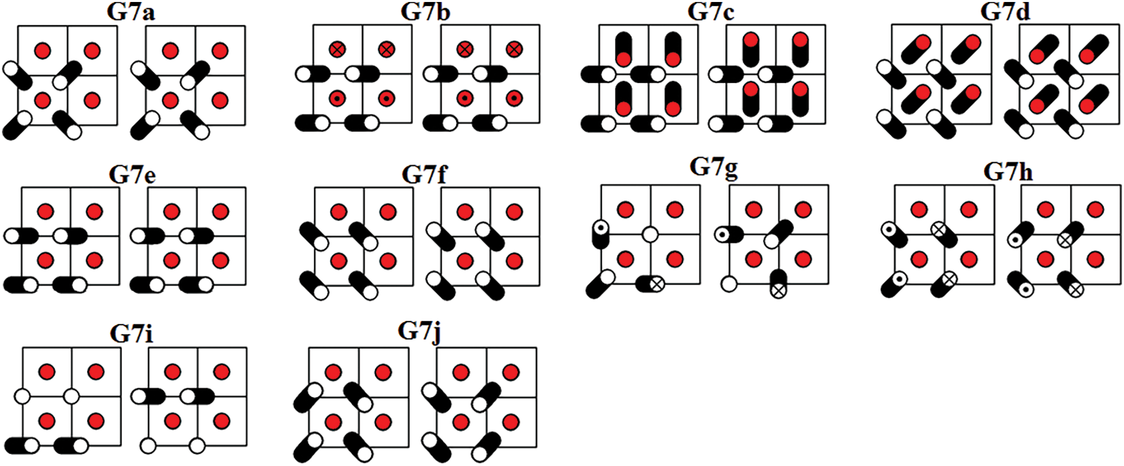
Figure 9: Ten DNVMs of group G7

The linear equations of motion of the bcc lattice have been obtained taking into account up to the fourth-neighbor interactions, see Eqs. (A6) to (A8). The phonon dispersion relation for the bcc lattice with long-range interactions has been derived, see Eq. (13) with the coefficients defined by Eqs. (11) and (12). The wavevectors of the DNVMs in the first Brillouin zone have been specified, see Table 1. The frequency response of the DNVMs in a wide range of vibration amplitude has been calculated numerically and plotted in Figs. 10 to 12.

Figure 10: Frequency response of DNVMs of groups G1, G2, and G3

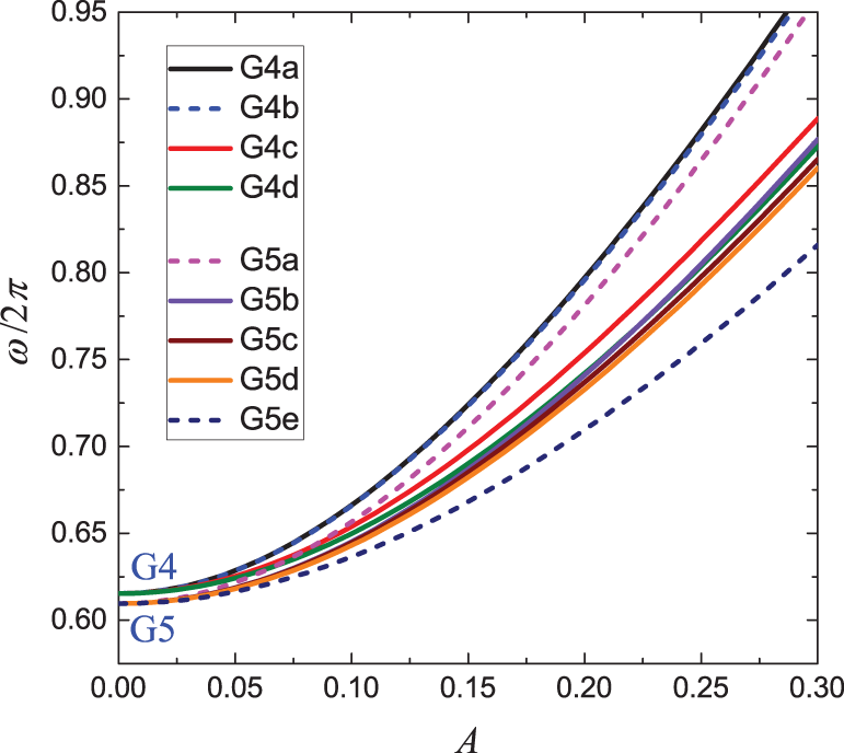
Figure 11: Frequency response of DNVMs of groups G4 and G5

Figure 12: Frequency response of DNVMs of groups G6 and G7

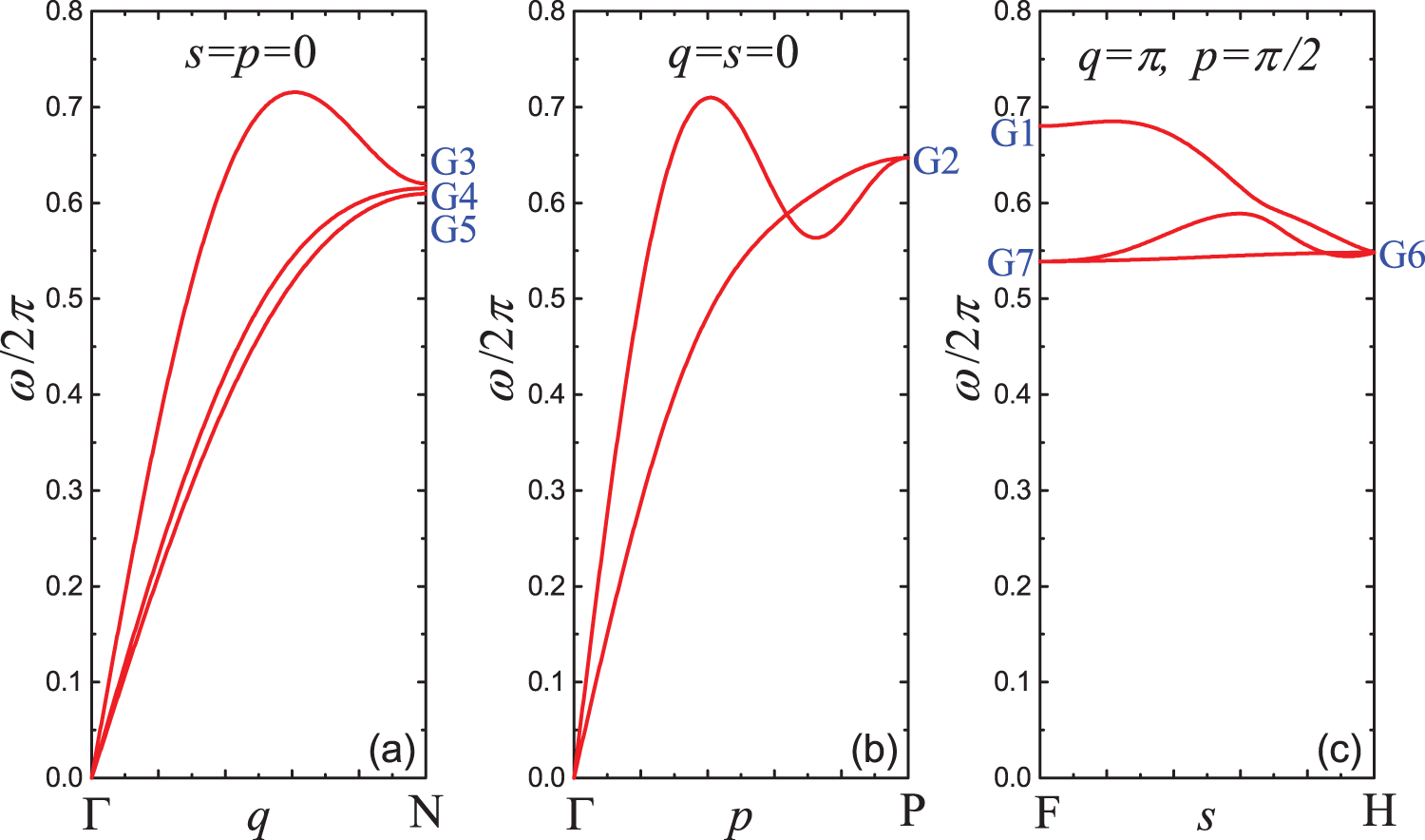
Figure 13: Dispersion curves along the high-symmetry lines of the first Brillouin zone: (a) s=p=0, (b) q=s=0, and (c) q=π, p=π/2

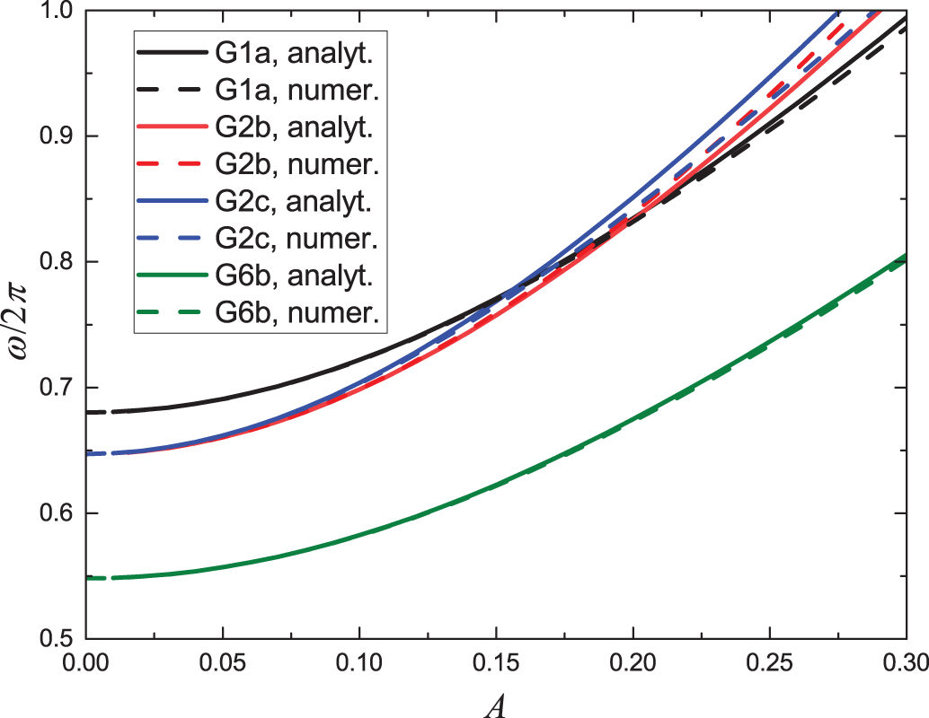
Figure 14: Frequency response for some DNVMs found numerically (solid lines) and analytically within the cubic approximation (dashed lines)

The frequencies of DNVMs in the small amplitude limit have been derived analytically, see Eq. (14) through Eq. (20). DNVMs are classified into seven groups according to their frequency in the small-amplitude limit. DNVMs belonging to one group deform interatomic bonds of different lengths equally in the harmonic approximation, see Table 2, but when anharmonicity comes into play, the potential energies stored by bonds of different lengths become different for DNVMs of the same group, see Table 3. Very important for testing and fitting the interatomic potentials is that different DNVMs test different types of bonds, as other types of bonds are not deformed or weakly deformed during the oscillation, see Tables 2 and 3. Several examples of analytical analysis of DNVMs are presented in Section 6. The frequency response of DNVMs obtained in the framework of the cubic approximation agrees well with the numerical results, see Fig. 14.

Let us describe the advantages and disadvantages of using DNVMs for testing and training interatomic potentials. The advantages are as follows:

1.   Small-amplitude DNVMs are the phonon modes. The high symmetry of DNVMs ensures that they do not interact with other phonon modes even at high vibration amplitudes so that the accuracy of the interatomic potentials can be assessed taking into account the effect of anharmonicity.

2.   DNVMs, as natural vibrational modes of the lattice, are recommended for testing and training interatomic potentials, as opposed to the use of random atomic configurations. Some of the random configurations may have a small probability of being realized, and therefore their contribution should be considered with a small weight, which is difficult to set because these probabilities are hard to estimate.

3.   DNVMs have a small translational cell, and their first-principles analysis using periodic boundary conditions is a routine task.

The disadvantages of DNVMs in testing and training of potentials include the following:

1.   DNVMs have a short wavelength and they do not test the potentials with respect to the long waves. To overcome this problem, homogeneous deformation of the crystal can be considered in addition to DNVMs.

2.   DNVMs do not provide information on crystal lattice defects. The defect configurations should be added to the training data set based on DNVMs.

The results obtained are important because they can be used to test the existing interatomic potentials and to develop new potentials for bcc crystals. The frequency response of the DNVMs calculated by first-principles modeling provides a rigorous test of the interatomic potentials. The DNVMs studied are the natural nonlinear vibrational modes of the bcc lattice and therefore any reliable interatomic potential must reproduce the frequency response of the DNVMs. The frequency response of the DNVMs can also be used to train the machine learning interatomic potentials. In the forthcoming work, DNVMs of fcc and hcp lattices will be studied, as there are many metals with these lattices.

Acknowledgement: Computational resources were provided by the Interdepartmental Supercomputer Center of the Russian Academy of Sciences.

Funding Statement: Igor V. Kosarev and Sergey V. Dmitriev acknowledge the support of the RSF Grant No. 24-11-00139 (analytics, numerical results, manuscript writing). Daxing Xiong acknowledges the support of the NNSF Grant No. 12275116, the NSF Grant No. 2021J02051, and the startup fund Grant No. MJY21035. For Aleksey A. Kudreyko, this work was supported by the Bashkir State Medical University Strategic Academic Leadership Program (PRIORITY-2030) (analytics).

Author Contributions: The authors contributed to the study as follows: conceptualization: Sergey V. Dmitriev; search for DNVMs: Denis S. Ryabov; simulations: Igor V. Kosarev; analysis and interpretation of results: Daxing Xiong, Sergey V. Dmitriev, Igor V. Kosarev, Aleksey A. Kudreyko; draft manuscript preparation: Sergey V. Dmitriev, Daxing Xiong. All authors reviewed the results and approved the final version of the manuscript.

Availability of Data and Materials: Data available on request from the authors.

Ethics Approval: Not applicable.

Conflicts of Interest: The authors declare no conflicts of interest to report regarding the present study.

Appendix A

Auxiliary Equations: The Hamiltonian Eq. (6) is the function of the following vectors connecting the atom i,j,k with its neighbors. The eight vectors connecting the particle i,j,k with its nearest neighbors are

Ri,j,k,1=ri,j,k−1−ri,j,k,Ri,j,k,2=ri,j,k+1−ri,j,k,Ri,j,k,3=ri+1,j,k−1−ri,j,k,Ri,j,k,4=ri−1,j,k+1−ri,j,k,Ri,j,k,5=ri+1,j+1,k−1−ri,j,k,Ri,j,k,6=ri−1,j−1,k+1−ri,j,k,Ri,j,k,7=ri,j+1,k−1−ri,j,k,Ri,j,k,8=ri,j−1,k+1−ri,j,k.(A1)

The six vectors connecting the particle i,j,k with its second neighbors are

Ri,j,k,9=ri−1,j,k−ri,j,k,Ri,j,k,10=ri+1,j,k−ri,j,k,Ri,j,k,11=ri,j−1,k−ri,j,k,Ri,j,k,12=ri,j+1,k−ri,j,k,Ri,j,k,13=ri+1,j+1,k−2−ri,j,k,Ri,j,k,14=ri−1,j−1,k+2−ri,j,k.(A2)

The twelve vectors connecting the particle i,j,k with its third neighbors are

Ri,j,k,15=ri−1,j−1,k−ri,j,k,Ri,j,k,16=ri+1,j+1,k−ri,j,k,Ri,j,k,17=ri+1,j−1,k−ri,j,k,Ri,j,k,18=ri−1,j+1,k−ri,j,k,Ri,j,k,19=ri+1,j,k−2−ri,j,k,Ri,j,k,20=ri−1,j,k+2−ri,j,k,Ri,j,k,21=ri+1,j+2,k−2−ri,j,k,Ri,j,k,22=ri−1,j−2,k+2−ri,j,k,Ri,j,k,23=ri,j+1,k−2−ri,j,k,Ri,j,k,24=ri,j−1,k+2−ri,j,k,Ri,j,k,25=ri+2,j+1,k−2−ri,j,k,Ri,j,k,26=ri−2,j−1,k+2−ri,j,k.(A3)

The twenty four vectors connecting the particle i,j,k with its fourth neighbors are

Ri,j,k,27=ri+1,j,k+1−ri,j,k,Ri,j,k,28=ri−1,j,k−1−ri,j,k,Ri,j,k,29=ri+1,j−1,k+1−ri,j,k,Ri,j,k,30=ri−1,j+1,k−1−ri,j,k,Ri,j,k,31=ri+2,j,k−1−ri,j,k,Ri,j,k,32=ri−2,j,k+1−ri,j,k,Ri,j,k,33=ri+2,j+1,k−1−ri,j,k,Ri,j,k,34=ri−2,j−1,k+1−ri,j,k,Ri,j,k,35=ri−1,j−1,k+3−ri,j,k,Ri,j,k,36=ri+1,j+1,k−3−ri,j,k,Ri,j,k,37=ri−2,j−1,k+3−ri,j,k,Ri,j,k,38=ri+2,j+1,k−3−ri,j,k,Ri,j,k,39=ri−1,j−2,k+3−ri,j,k,Ri,j,k,40=ri+1,j+2,k−3−ri,j,k,Ri,j,k,41=ri−2,j−2,k+3−ri,j,k,Ri,j,k,42=ri+2,j+2,k−3−ri,j,k,Ri,j,k,43=ri,j+1,k+1−ri,j,k,Ri,j,k,44=ri,j−1,k−1−ri,j,k,Ri,j,k,45=ri−1,j+1,k+1−ri,j,k,Ri,j,k,46=ri+1,j−1,k−1−ri,j,k,Ri,j,k,47=ri+1,j+2,k−1−ri,j,k,Ri,j,k,48=ri−1,j−2,k+1−ri,j,k,Ri,j,k,49=ri,j+2,k−1−ri,j,k,Ri,j,k,50=ri,j−2,k+1−ri,j,k.(A4)

Linearized equations of motion can be derived from Eq. (7) assuming that |uij|,|vij|,|wij|≪h. The following second-order finite difference operators are introduced to shorten the equations:

Δ2ui+a,j+b,k+c=ui+a,j+b,k+c−2ui,j,k+ui−a,j−b,k−c,Δ2vi+a,j+b,k+c=vi+a,j+b,k+c−2vi,j,k+vi−a,j−b,k−c,Δ2wi+a,j+b,k+c=wi+a,j+b,k+c−2wi,j,k+wi−a,j−b,k−c.(A5)

The linear equations of motion are

mu¨i,j,k=c13Δ2ui,j,k−1+c13Δ2vi,j,k−1+c13Δ2wi,j,k−1+c13Δ2ui+1,j,k−1−c13Δ2vi+1,j,k−1−c13Δ2wi+1,j,k−1+c13Δ2ui+1,j+1,k−1+c13Δ2vi+1,j+1,k−1−c13Δ2wi+1,j+1,k−1+c13Δ2ui,j+1,k−1−c13Δ2vi,j+1,k−1+c13Δ2wi,j+1,k−1+c2Δ2ui−1,j,k+c32Δ2ui−1,j−1,k+c32Δ2vi−1,j−1,k+c32Δ2ui+1,j−1,k−c32Δ2vi+1,j−1,k+c32Δ2ui,j+1,k−2+c32Δ2wi,j+1,k−2+c32Δ2ui+2,j+1,k−2−c32Δ2wi+2,j+1,k−2+9c411Δ2ui+1,j,k+1+3c411Δ2vi+1,j,k+1+3c411Δ2wi+1,j,k+1+9c411Δ2ui+1,j−1,k+1−3c411Δ2vi+1,j−1,k+1+3c411Δ2wi+1,j−1,k+1+9c411Δ2ui+2,j,k−1−3c411Δ2vi+2,j,k−1−3c411Δ2wi+2,j,k−1+9c411Δ2ui+2,j+1,k−1+3c411Δ2vi+2,j+1,k−1−3c411Δ2wi+2,j+1,k−1+c411Δ2ui−1,j−1,k+3+c411Δ2vi−1,j−1,k+3+3c411Δ2wi−1,j−1,k+3+c411Δ2ui−2,j−1,k+3−c411Δ2vi−2,j−1,k+3−3c411Δ2wi−2,j−1,k+3+c411Δ2ui−1,j−2,k+3−c411Δ2vi−1,j−2,k+3+3c411Δ2wi−1,j−2,k+3+c411Δ2ui−2,j−2,k+3+c411Δ2vi−2,j−2,k+3−3c411Δ2wi−2,j−2,k+3+c411Δ2ui,j+1,k+1+3c411Δ2vi,j+1,k+1+c411Δ2wi,j+1,k+1+c411Δ2ui−1,j+1,k+1−3c411Δ2vi−1,j+1,k+1−c411Δ2wi−1,j+1,k+1+c411Δ2ui+1,j+2,k−1+3c411Δ2vi+1,j+2,k−1−c411Δ2wi+1,j+2,k−1+c411Δ2ui,j+2,k−1−3c411Δ2vi,j+2,k−1+c411Δ2wi,j+2,k−1,(A6)

References

1. Wen T, Zhang L, Wang H, Weinan E, Srolovitz DJ. Deep potentials for materials science. Mater Futures. 2022;1(2):022601. doi:10.1088/2752-5724/ac681d. [Google Scholar] [CrossRef]
2. Wang F, Wu HH, Dong L, Pan G, Zhou X, Wang S, et al. Atomic-scale simulations in multi-component alloys and compounds: a review on advances in interatomic potential. J Mater Sci Technol. 2023;165:49–65. doi:10.1016/j.jmst.2023.05.010. [Google Scholar] [CrossRef]
3. Martin-Barrios R, Navas-Conyedo E, Zhang X, Chen Y, Gulin-Gonzalez J. An overview about neural networks potentials in molecular dynamics simulation. Int J Quantum Chem. 2024;124(11):e27389. doi:10.1002/qua.27389. [Google Scholar] [CrossRef]
4. Kocer E, Ko TW, Behler J. Neural network potentials: a concise overview of methods. Annu Rev Phys Chem. 2022;73(1):163–86. doi:10.1146/annurev-physchem-082720-034254. [Google Scholar] [PubMed] [CrossRef]
5. Yang Y, Zhang S, Ranasinghe KD, Isayev O, Roitberg AE. Machine learning of reactive potentials. Annu Rev Phys Chem. 2024;75(1):371–95. doi:10.1146/annurev-physchem-062123-024417. [Google Scholar] [CrossRef]
6. Urata S, Bertani M, Pedone A. Applications of machine-learning interatomic potentials for modeling ceramics, glass, and electrolytes: a review. J Am Ceram Soc. 2024;107(12):7665–91. doi:10.1111/jace.19934. [Google Scholar] [CrossRef]
7. Smith JS, Isayev O, Roitberg AE. ANI-1: an extensible neural network potential with DFT accuracy at force field computational cost. Chem Sci. 2017;8(4):3192–203. doi:10.1039/C6SC05720A. [Google Scholar] [PubMed] [CrossRef]
8. Naghdi AD, Pellegrini F, Kucukbenli E, Massa D, Dominguez-Gutierrez FJ, Kaxiras E, et al. Neural network interatomic potentials for open surface nano-mechanics applications. Acta Mater. 2024;277(17):120200. doi:10.1016/j.actamat.2024.120200. [Google Scholar] [CrossRef]
9. Zotov N, Gubaev K, Worner J, Grabowski B. Moment tensor potential for static and dynamic investigations of screw dislocations in bcc Nb. Model Simul Mater Sci Eng. 2024;32(3):035032. doi:10.1088/1361-651X/ad2d68. [Google Scholar] [CrossRef]
10. Aitken ZH, Sorkin V, Gen Yu Z, Chen S, Leong Tan T, Wu Z, et al. Controlling screw dislocation core structure and Peierls barrier in BCC interatomic potentials. Int J Solids Struct. 2024;303:113004. doi:10.1016/j.ijsolstr.2024.113004. [Google Scholar] [CrossRef]
11. Romaner L, Pradhan T, Kholtobina A, Drautz R, Mrovec M. Theoretical investigation of the 70.5° mixed dislocations in body-centered cubic transition metals. Acta Mater. 2021;217:117154. doi:10.1016/j.actamat.2021.117154. [Google Scholar] [CrossRef]
12. Bertin N, Cai W, Aubry S, Bulatov VV. Core energies of dislocations in bcc metals. Phys Rev Mater. 2021;5(2):025002. doi:10.1103/PhysRevMaterials.5.025002. [Google Scholar] [CrossRef]
13. Suzudo T, Ki Ebihara, Tsuru T, Mori H. Cleavages along {110} in bcc iron emit dislocations from the curved crack fronts. Sci Rep. 2022;12(1):19701. doi:10.1038/s41598-022-24357-5. [Google Scholar] [CrossRef]
14. Maksimenko VN, Lipnitskii AG, Saveliev VN, Nelasov IV, Kartamyshev AI. Prediction of the diffusion characteristics of the V-Cr system by molecular dynamics based on N-body interatomic potentials. Comput Mater Sci. 2021;198:110648. doi:10.1016/j.commatsci.2021.110648. [Google Scholar] [CrossRef]
15. Konov DA, Sidnov KP, Sinyakov RI, Belov MP. Effect of deformation on the diffusion properties of β-Zr at high temperatures. Phys Met Metallography. 2024;125(8):843–50. doi:10.1134/S0031918X24601173. [Google Scholar] [CrossRef]
16. Magomedov MN. Parameters of the vacancy formation and self-diffusion in the iron. J Phys Chem Solids. 2023;172(1):111084. doi:10.1016/j.jpcs.2022.111084. [Google Scholar] [CrossRef]
17. Yuan XJ, Chen NX, Shen J. Construction of embedded-atom-method interatomic potentials for alkaline metals (Li, Na, and K) by lattice inversion. Chin Phys B. 2012;21(5):053401. doi:10.1088/1674-1056/21/5/053401. [Google Scholar] [CrossRef]
18. Suzudo T, Ebihara KI, Tsuru T, Mori H. Large-scale atomislic simulations of cleavage in BCC Fe using machine-learning potential. Zairyo/J Soc Mat Sci. 2024;73(2):129–35. doi:10.2472/jsms.73.129. [Google Scholar] [CrossRef]
19. Zhang M, Hibi K, Inoue J. Highly accurate and efficient potential for bcc iron assisted by artificial neural networks. Phys Rev B. 2024;110(5):054110. doi:10.1103/PhysRevB.110.054110. [Google Scholar] [CrossRef]
20. Wang R, Ma X, Zhang L, Wang H, Srolovitz DJ, Wen T, et al. Classical and machine learning interatomic potentials for BCC vanadium. Phys Rev Mater. 2022;6(11):113603. doi:10.1103/PhysRevMaterials.6.113603. [Google Scholar] [CrossRef]
21. Goryaeva AM, Deres J, Lapointe C, Grigorev P, Swinburne TD, Kermode JR, et al. Efficient and transferable machine learning potentials for the simulation of crystal defects in bcc Fe and W. Phys Rev Mater. 2021;5(10):103803. doi:10.1103/PhysRevMaterials.5.103803. [Google Scholar] [CrossRef]
22. Kazakov A, Babicheva RI, Zinovev A, Terentyev D, Zhou K, Korznikova EA, et al. Interaction of edge dislocations with voids in tungsten. Tungsten. 2024;6(3):633–46. doi:10.1007/s42864-023-00250-0. [Google Scholar] [CrossRef]
23. Kramynin SP. Theoretical study of the size dependencies of the thermodynamic properties of tungsten at various pressures and temperatures. J Phys Chem Solids. 2021;152(3):109964. doi:10.1016/j.jpcs.2021.109964. [Google Scholar] [CrossRef]
24. Lin YS, Pun GPP, Mishin Y. Development of a physically-informed neural network interatomic potential for tantalum. Comput Mater Sci. 2022;205(148):111180. doi:10.1016/j.commatsci.2021.111180. [Google Scholar] [CrossRef]
25. Yin WQ, Bo T, Zhao YB, Zhang L, Chai ZF, Shi WQ. Deep learning of accurate interatomic potentials for uranium, zirconium and uranium-zirconium alloy. He-Huaxue Yu Fangshe Huaxue/J Nucl Radiochem. 2024;46(5):450–61. [Google Scholar]
26. Slooter RJ, Sluiter MHF, Kranendonk WGT, Bos C. A reference-free MEAM potential for α-Fe and γ-Fe. J Phys Condens Matter. 2022;34(50):505901. doi:10.1088/1361-648X/ac9d14. [Google Scholar] [PubMed] [CrossRef]
27. Xue HT, Li J, Chang Z, Yang YH, Tang FL, Zhang Y, et al. Deep-learning potential molecular dynamics simulations of the structural and physical properties of rare-earth metal scandium. Comput Mater Sci. 2024;242:113072. doi:10.1016/j.commatsci.2024.113072. [Google Scholar] [CrossRef]
28. Qin Z, Wang R, Li S, Wen T, Yin B, Wu Z. MEAM interatomic potential for thermodynamic and mechanical properties of lithium allotropes. Comput Mater Sci. 2022;214:111706. doi:10.1016/j.commatsci.2022.111706. [Google Scholar] [CrossRef]
29. Jian Z, Chen Y, Xiao S, Wang L, Li X, Wang K, et al. Shock-induced plasticity and phase transformation in single crystal magnesium: an interatomic potential and non-equilibrium molecular dynamics simulations. J Phys Condens Matter. 2022;34(11):115401. doi:10.1088/1361-648X/ac443e. [Google Scholar] [PubMed] [CrossRef]
30. Ji H, Wang Y, Yin J, Hou H, Lai W, Mei J, et al. Comparison of interatomic potentials on crack propagation properties in bcc iron. Int J Press Vessel Piping. 2021;194:104524. doi:10.1016/j.ijpvp.2021.104524. [Google Scholar] [CrossRef]
31. Sajad Mousavi Nejad Souq S, Ashenai Ghasemi F, Masoud Seyyed Fakhrabadi M. Performance of different traditional and machine learning-based atomistic potential functions in the simulation of mechanical behavior of Fe nanowires. Comput Mater Sci. 2022;215(7):111807. doi:10.1016/j.commatsci.2022.111807. [Google Scholar] [CrossRef]
32. Hou J, You YW, Kong XS, Song J, Liu CS. Accurate prediction of vacancy cluster structures and energetics in bcc transition metals. Acta Mater. 2021;211:116860. doi:10.1016/j.actamat.2021.116860. [Google Scholar] [CrossRef]
33. Faisal AHM, Weinberger CR. Modeling twin boundary structures in body centered cubic transition metals. Comput Mater Sci. 2021;197:110649. doi:10.1016/j.commatsci.2021.110649. [Google Scholar] [CrossRef]
34. Manna M, Pal S. Investigation of primary radiation damage in nanocrystalline tantalum using machine-learning interatomic potential: an atomistic simulation study. In: Advances in risk and reliability modelling and assessment. Singapore: Springer; 2024;167–82. doi:10.1007/978-981-97-3087-2. [Google Scholar] [CrossRef]
35. Wang Y, Liu J, Li J, Mei J, Li Z, Lai W, et al. Machine-learning interatomic potential for radiation damage effects in bcc-iron. Comput Mater Sci. 2022;202:110960. doi:10.1016/j.commatsci.2021.110960. [Google Scholar] [CrossRef]
36. Magomedov MN. Calculation of the surface energy of a crystal and its temperature and pressure dependence. J Surf Investig. 2020;14(6):1208–20. doi:10.1134/s1027451020060105. [Google Scholar] [CrossRef]
37. Zhang L, Csanyi G, van der Giessen E, Maresca F. Atomistic fracture in bcc iron revealed by active learning of Gaussian approximation potential. npj Comp Mater. 2023;9(1):217. doi:10.1038/s41524-023-01174-6. [Google Scholar] [CrossRef]
38. Sun H, Samanta A. Exploring structural transitions at grain boundaries in Nb using a generalized embedded atom interatomic potential. Comput Mater Sci. 2023;230:112497. doi:10.1016/j.commatsci.2023.112497. [Google Scholar] [CrossRef]
39. French J, Bai XM. Molecular dynamics studies of grain boundary mobility and anisotropy in BCC γ-uranium. J Nucl Mater. 2022;565:153744. doi:10.1016/j.jnucmat.2022.153744. [Google Scholar] [CrossRef]
40. Oren E, Kartoon D, Makov G. Machine learning-based modeling of high-pressure phase diagrams: anomalous melting of Rb. J Chem Phys. 2022;157(1):014502. doi:10.1063/5.0088089. [Google Scholar] [CrossRef]
41. Kotykhov AS, Gubaev K, Hodapp M, Tantardini C, Shapeev AV, Novikov IS. Constrained DFT-based magnetic machine-learning potentials for magnetic alloys: a case study of Fe-Al. Sci Rep. 2023;13(1):19728. doi:10.1038/s41598-023-46951-x. [Google Scholar] [CrossRef]
42. Novikov I, Grabowski B, Kormann F, Shapeev A. Magnetic moment tensor potentials for collinear spin-polarized materials reproduce different magnetic states of bcc Fe. npj Comp Mater. 2022;8(1):13. doi:10.1038/s41524-022-00696-9. [Google Scholar] [CrossRef]
43. Chapman JBJ, Ma PW. A machine-learned spin-lattice potential for dynamic simulations of defective magnetic iron. Sci Rep. 2022;12(1):22451. doi:10.1038/s41598-022-25682-5. [Google Scholar] [PubMed] [CrossRef]
44. Akhunova AK, Murzaev RT, Baimova JA. Graphene with dislocation dipoles: wrinkling and defect nucleation during tension. Comput Mater Sci. 2024;244(5887):113230. doi:10.1016/j.commatsci.2024.113230. [Google Scholar] [CrossRef]
45. Safina LR, Krylova KA, Murzaev RT, Shcherbinin SA, Baimova JA. Graphene/Ni composite coating for enhanced strength of Ni surface. Surf Interfaces. 2024;53(18):105011. doi:10.1016/j.surfin.2024.105011. [Google Scholar] [CrossRef]
46. Polyakova PV, Murzaev RT, Lisovenko DS, Baimova JA. Elastic constants of graphane, graphyne, and graphdiyne. Comput Mater Sci. 2024;244:113171. doi:10.1016/j.commatsci.2024.113171. [Google Scholar] [CrossRef]
47. Safina LR, Rozhnova EA, Krylova KA, Murzaev RT, Baimova JA. Interatomic potentials for graphene reinforced metal composites: optimal choice. Comput Phys Commun. 2024;301:109235. doi:10.1016/j.cpc.2024.109235. [Google Scholar] [CrossRef]
48. Chen X, Wang LF, Gao XY, Zhao YF, Lin DY, Chu WD, et al. Machine learning enhanced empirical potentials for metals and alloys. Comput Phys Commun. 2021;269:108132. doi:10.1016/j.cpc.2021.108132. [Google Scholar] [CrossRef]
49. Shapeev AV, Podryabinkin EV, Gubaev K, Tasnadi F, Abrikosov IA. Elinvar effect in β-Ti simulated by on-the-fly trained moment tensor potential. New J Phys. 2020;22(11):113005. doi:10.1088/1367-2630/abc392. [Google Scholar] [CrossRef]
50. Dickel D, Nitol M, Barrett CD. LAMMPS implementation of rapid artificial neural network derived interatomic potentials. Comput Mater Sci. 2021;196:110481. doi:10.1016/j.commatsci.2021.110481. [Google Scholar] [CrossRef]
51. Poul M, Huber L, Bitzek E, Neugebauer J. Systematic atomic structure datasets for machine learning potentials: application to defects in magnesium. Phys Rev B. 2023;107(10):104103. doi:10.1103/PhysRevB.107.104103. [Google Scholar] [CrossRef]
52. Dmitriev SV, Kistanov AA, Kosarev IV, Scherbinin SA, Shapeev AV. Construction of machine learning interatomic potentials for metals. Russ Phys J. 2024;67(9):1408–13. doi:10.1007/s11182-024-03261-7. [Google Scholar] [CrossRef]
53. Ryabov DS, Bezuglova GS, Korznikova EA, Dmitriev SV. Testing interatomic potentials for binary alloys using exact solutions to the equations of atomic motion. Procedia Struct Integr. 2024;65(11):209–14. doi:10.1016/j.prostr.2024.11.032. [Google Scholar] [CrossRef]
54. Chechin GM, Dzhelauhova GS. Discrete breathers and nonlinear normal modes in monoatomic chains. J Sound Vib. 2009 May;322(3):490–512. doi:10.1016/j.jsv.2008.04.002. [Google Scholar] [CrossRef]
55. Chechin G, Bezuglova G. Resonant excitation of the bushes of nonlinear vibrational modes in monoatomic chains. Commun Nonlinear Sci. 2023;126(6):107509. doi:10.1016/j.cnsns.2023.107509. [Google Scholar] [CrossRef]
56. Chechin GM, Sizintsev DA, Usoltsev OA. Nonlinear atomic vibrations and structural phase transitions in strained carbon chains. Comp Mater Sci. 2017;138(19):353–67. doi:10.1016/j.commatsci.2017.07.004. [Google Scholar] [CrossRef]
57. Chechin GM, Shcherbinin SA. Delocalized periodic vibrations in nonlinear LC and LCR electrical chains. Commun Nonlinear Sci. 2015;22(1–3):244–62. doi:10.1016/j.cnsns.2014.09.028. [Google Scholar] [CrossRef]
58. Rosenberg RM. The normal modes of nonlinear n-degree-of-freedom systems. J Appl Mech T ASME. 1960;29(1):7–14. doi:10.1115/1.3636501. [Google Scholar] [CrossRef]
59. Ryabov DS, Chechin GM, Upadhyaya A, Korznikova EA, Dubinko VI, Dmitriev SV. Delocalized nonlinear vibrational modes of triangular lattices. Nonlinear Dyn. 2020;102(4):2793–810. doi:10.1007/s11071-020-06015-5. [Google Scholar] [CrossRef]
60. Ryabov DS, Chechin GM, Naumov EK, Bebikhov YV, Korznikova EA, Dmitriev SV. One-component delocalized nonlinear vibrational modes of square lattices. Nonlinear Dyn. 2023;111(9):8135–53. doi:10.1007/s11071-023-08264-6. [Google Scholar] [CrossRef]
61. Shcherbinin SA, Kazakov AM, Bebikhov YV, Kudreyko AA, Dmitriev SV. Delocalized nonlinear vibrational modes and discrete breathers in β-FPUT simple cubic lattice. Phys Rev E. 2024;109(1):014215. doi:10.1103/PhysRevE.109.014215. [Google Scholar] [PubMed] [CrossRef]
62. Shcherbinin SA, Krylova KA, Chechin GM, Soboleva EG, Dmitriev SV. Delocalized nonlinear vibrational modes in fcc metals. Commun Nonlinear Sci. 2022;104:106039. doi:10.1016/j.cnsns.2021.106039. [Google Scholar] [CrossRef]
63. Shcherbinin SA, Bebikhov YV, Abdullina DU, Kudreyko AA, Dmitriev SV. Delocalized nonlinear vibrational modes and discrete breathers in a body centered cubic lattice. Commun Nonlinear Sci. 2024;135:108033. doi:10.1016/j.cnsns.2024.108033. [Google Scholar] [CrossRef]
64. Bezuglova GS, Chechin GM, Goncharov PP. Discrete breathers on symmetry-determined invariant manifolds for scalar models on the plane square lattice. Phys Rev E. 2011;84(3):036606. doi:10.1103/PhysRevE.84.036606. [Google Scholar] [PubMed] [CrossRef]
65. Ilgamov MA, Aitbaeva AA, Pavlov IS, Dmitriev SV. Carbon nanotube under pulsed pressure. Facta Univ, Ser: Mech Eng. 2024;22(2):275–92. doi:10.22190/FUME230820049I. [Google Scholar] [CrossRef]
66. Bachurina OV, Murzaev RT, Shcherbinin SA, Kudreyko AA, Dmitriev SV, Bachurin DV. Delocalized nonlinear vibrational modes in Ni3Al. Commun Nonlinear Sci. 2024;132:107890. doi:10.1016/j.cnsns.2024.107890. [Google Scholar] [CrossRef]
67. Bachurina OV, Kudreyko AA. Two-dimensional discrete breathers in fcc metals. Comp Mater Sci. 2020;182:109737. doi:10.1016/j.commatsci.2020.109737. [Google Scholar] [CrossRef]
68. Bachurina OV. Linear discrete breather in fcc metals. Comp Mater Sci. 2019;160:217–21. doi:10.1016/j.commatsci.2019.01.014. [Google Scholar] [CrossRef]
69. Bachurina OV, Murzaev RT, Bachurin DV. Molecular dynamics study of two-dimensional discrete breather in nickel. J Micromech Mol Phys. 2019;4(2):1950001. doi:10.1142/S2424913019500012. [Google Scholar] [CrossRef]
70. Bachurina OV. Plane and plane-radial discrete breathers in fcc metals. Model Simul Mater Sc. 2019;27(5):055001. doi:10.1088/1361-651X/ab17b7. [Google Scholar] [CrossRef]
71. Kosarev IV, Shcherbinin SA, Kistanov AA, Babicheva RI, Korznikova EA, Dmitriev SV. An approach to evaluate the accuracy of interatomic potentials as applied to tungsten. Comp Mater Sci. 2024;231(1):112597. doi:10.1016/j.commatsci.2023.112597. [Google Scholar] [CrossRef]
72. Cuevas J, Archilla JFR, Gaididei YB, Romero FR. Moving breathers in a DNA model with competing short-and long-range dispersive interactions. Physica D. 2002;163(1–2):106–26. doi:10.1016/S0167-2789(02)00351-2. [Google Scholar] [CrossRef]
73. Gorbach AV, Flach S. Compactlike discrete breathers in systems with nonlinear and nonlocal dispersive terms. Phys Rev E. 2005;72(5):056607. doi:10.1103/PhysRevE.72.056607. [Google Scholar] [PubMed] [CrossRef]
74. Koukouloyannis V, Kevrekidis PG, Cuevas J, Rothos V. Multibreathers in Klein-gordon chains with interactions beyond nearest neighbors. Physica D. 2013;242(1):16–29. doi:10.1016/j.physd.2012.08.011. [Google Scholar] [CrossRef]
75. Gninzanlong CL, Ndjomatchoua FT, Tchawoua C. Forward and backward propagating breathers in a DNA model with dipole-dipole long-range interactions. Phys Rev E. 2020;102(5):052212. doi:10.1103/PhysRevE.102.052212. [Google Scholar] [PubMed] [CrossRef]
76. Christodoulidi H, Bountis A, Drossos L. The effect of long-range interactions on the dynamics and statistics of 1D Hamiltonian lattices with on-site potential. Eur Phys J Spec Top. 2018;227(5–6):563–73. doi:10.1140/epjst/e2018-00003-9. [Google Scholar] [CrossRef]
77. Bonart D. Intrinsic localized modes in linear chains with Coulomb interaction. Phys Lett A. 1997;231(3–4):201–7. doi:10.1016/S0375-9601(97)00298-3. [Google Scholar] [CrossRef]
78. Bonart D, Rossler T, Page JB. Intrinsic localized modes in complex lattice dynamical systems. Physica D. 1998;113(2–4):123–8. doi:10.1016/S0167-2789(97)00259-5. [Google Scholar] [CrossRef]
79. Kevrekidis PG, Gaididei YB, Bishop AR, Saxena A. Effects of competing short- and long-range dispersive interactions on discrete breathers. Phys Rev E. 2001;64:66606/1–8. doi:10.1103/PhysRevE.64.066606. [Google Scholar] [PubMed] [CrossRef]
80. Bagchi D. Energy transport in the presence of long-range interactions. Phys Rev E. 2017;96(4):042121. doi:10.1103/PhysRevE.96.042121. [Google Scholar] [PubMed] [CrossRef]
81. Iubini S, Di Cintio P, Lepri S, Livi R, Casetti L. Heat transport in oscillator chains with long-range interactions coupled to thermal reservoirs. Phys Rev E. 2018;97(3):032102. doi:10.1103/PhysRevE.97.032102. [Google Scholar] [PubMed] [CrossRef]
82. Doi Y, Yoshimura K. Construction of nonlinear lattice with potential symmetry for smooth propagation of discrete breather. Nonlinearity. 2020;33(10):5142–75. doi:10.1088/1361-6544/ab9498. [Google Scholar] [CrossRef]
83. Yamaguchi YY, Doi Y. Low-frequency discrete breathers in long-range systems without on-site potential. Phys Rev E. 2018;97(6):062218. doi:10.1103/PhysRevE.97.062218. [Google Scholar] [CrossRef]
84. Xie Y, Zhang JM. Atomistic simulation of phonon dispersion for body-centred cubic alkali metals. Can J Phys. 2008;86(6):801–5. doi:10.1139/p07-200. [Google Scholar] [CrossRef]
85. Wilson RB, Riffe DM. An embedded-atom-method model for alkali-metal vibrations. J Phys Condens Mat. 2012;24(33):335401. doi:10.1088/0953-8984/24/33/335401. [Google Scholar] [PubMed] [CrossRef]
86. Jong GB, Song P, Jin HS. Phonon and thermodynamic properties of bcc transition metals using MEAM potentials. Indian J Phys. 2020;94(6):753–66. doi:10.1007/s12648-019-01497-5. [Google Scholar] [CrossRef]
87. Mei H, Wang F, Li J, Kong L. Elastic anisotropy and its temperature dependence for cubic crystals revealed by molecular dynamics simulations. Model Simul Mater Sc. 2023;31(6):065013. doi:10.1088/1361-651X/ace541. [Google Scholar] [CrossRef]
88. Geshi M, Funashima H, Hettiarachchi GP. First-principles study of highly-compressed Sb: a stubborn body-centered cubic structure. Jpn J Appl Phys. 2022;61(8):012011. doi:10.35848/1347-4065/ac8035. [Google Scholar] [CrossRef]
89. Troncoso JF, Turlo V. Evaluating the applicability of classical and neural network interatomic potentials for modeling body centered cubic polymorph of magnesium. Model Simul Mater Sc. 2022;30(4):045009. doi:10.1088/1361-651X/ac5ebc. [Google Scholar] [CrossRef]
90. Qian X, Yang R. Temperature effect on the phonon dispersion stability of zirconium by machine learning driven atomistic simulations. Phys Rev B. 2018;98(22):224108. doi:10.1103/PhysRevB.98.224108. [Google Scholar] [CrossRef]
91. Pandey P, Pandey SK. Ab initio investigation of the lattice dynamics and thermophysical properties of bcc vanadium and niobium. J Phys Condens Mat. 2024;36(16):165602. doi:10.1088/1361-648X/ad1bf4. [Google Scholar] [PubMed] [CrossRef]
92. Bakhvalov NS. Numerical methods: analysis, algebra, ordinary differential equations. Moscow: MIR Publishers; 1977. [Google Scholar]
93. Chechin GM, Sakhnenko VP. Interactions between normal modes in nonlinear dynamical systems with discrete symmetry. Exact results. Physica D. 1998;117(1–4):43–76. doi:10.1016/S0167-2789(98)80012-2. [Google Scholar] [CrossRef]
Cite This Article
Copyright © 2025 The Author(s). Published by Tech Science Press.
This work is licensed under a Creative Commons Attribution 4.0 International License , which permits unrestricted use, distribution, and reproduction in any medium, provided the original work is properly cited.
Downloads
Citation Tools