
 Submit a Paper
 Propose a Special lssue
 Open Access
ARTICLE
Utilizing Machine Learning and SHAP Values for Improved and Transparent Energy Usage Predictions
1 School of Electrical and Electronic Engineering, Universiti Sains Malaysia, Seberang Perai, 14300, Malaysia
2 Electrical Engineering Department, Tikrit University, Tikrit, 34001, Iraq
3 Department of Electrical and Computer Engineering, College of Engineering and Information Technology, Ajman University, Ajman, P.O. Box 346, United Arab Emirates
* Corresponding Author: Abdul Sattar Din. Email:
Computers, Materials & Continua 2025, 83(2), 3553-3583. https://doi.org/10.32604/cmc.2025.061400
Received 23 November 2024; Accepted 03 March 2025; Issue published 16 April 2025
 View Full Text
 Download PDF
Abstract
The significance of precise energy usage forecasts has been highlighted by the increasing need for sustainability and energy efficiency across a range of industries. In order to improve the precision and openness of energy consumption projections, this study investigates the combination of machine learning (ML) methods with Shapley additive explanations (SHAP) values. The study evaluates three distinct models: the first is a Linear Regressor, the second is a Support Vector Regressor, and the third is a Decision Tree Regressor, which was scaled up to a Random Forest Regressor/Additions made were the third one which was Regressor which was extended to a Random Forest Regressor. These models were deployed with the use of Shareable, Plot-interpretable Explainable Artificial Intelligence techniques, to improve trust in the AI. The findings suggest that our developed models are superior to the conventional models discussed in prior studies; with high Mean Absolute Error (MAE) and Root Mean Squared Error (RMSE) values being close to perfection. In detail, the Random Forest Regressor shows the MAE of 0.001 for predicting the house prices whereas the SVR gives 0.21 of MAE and 0.24 RMSE. Such outcomes reflect the possibility of optimizing the use of the promoted advanced AI models with the use of Explainable AI for more accurate prediction of energy consumption and at the same time for the models’ decision-making procedures’ explanation. In addition to increasing prediction accuracy, this strategy gives stakeholders comprehensible insights, which facilitates improved decision-making and fosters confidence in AI-powered energy solutions. The outcomes show how well ML and SHAP work together to enhance prediction performance and guarantee transparency in energy usage projections.Keywords
Abbreviations
| MAE | Mean Absolute Error |
| RMSE | Root Mean Squared Error |
| IEA | International Energy Agency |
| ML | Machine Learning |
| DL | Deep Learning |
| MLR | Multiple Linear Regression |
| GBM | Gradient Boosting Machines |
| RF | Random Forest |
| CNN | Convolutional Neural Networks |
| LSTM | Long Short-Term Memory |
| ESAT | Experimental Self-Attention Transformer |
| SVM | Support Vector Machine |
| SVR | Support Vector Regression |
| SHAP | SHapley Additive exPlanations |
Over the last couple of decades, energy consumption has sharply increased along with the growth of industrial and commercial segments. The industrialization process has recorded impressive growth in sectors such as economy and population across the globe. Therefore, energy is commonly deemed as one of the key determinants of national progress and can affect the decisions in many states [1]. However, there are challenges that the energy sector is facing, which include the need to promote economic development, energy security, and greenhouse emissions. According to the International Energy Agency (IEA), different measures can be implemented to solve the aforementioned challenges like advanced energy usage forecasting models [2]. These models help in predicting future energy demand, the effects of any policy changes, and the viability of different energy technologies to facilitate the shift to a sustainable energy system [3].
Manufacturing consumes electricity in the commercial sector. In 2021, the United States consumed about a third of all energy in industrial activities [4]. In 1988, a total of 1.753 million metric tons of carbon was released into the atmosphere as a byproduct of energy production [5]. Power needs to be lowered by major consumers in a direct attempt to decrease emissions from their generation. This sector domestically uses nearly one-third of all energy in the US, while industrial emissions account for over 25% of total U.S. energy-related emissions. By 2050, emissions from space cooling are expected to increase at a faster rate than any other end-use [6]. Thus, it is essential to decrease energy usage and the emissions stemming from this sector at large. On a global scale, the commercial and residential sectors were responsible for around 34.7% of the total energy use. A reliable prediction of energy demand in these categories can help governments manage their allocations and formulate plans for clean and sustainable energy. This includes a combination of non-renewable and renewable energy sources to produce an unbreakable, environmentally friendly, and intelligent energy system [7,8]. The hierarchical structure of this paper is well laid down to ensure that the reader comprehensively understands the utilization of machine learning to forecast renewable energy consumption as well as the creative use of SHAP values for explainability. The paper is organized into several main sections that are intended to provide a comprehensive analysis and discussion of the findings.
The first section, after this preface, includes the literature review in which we present and discuss the state of the art in the use of machine learning techniques in energy forecasting. Besides, this review also outlines what has been done and not been done with the existing methodologies, which serves as the foundation to introduce SHAP values as a new explainability method. This section compares existing techniques with the recent developments to emphasize on increasing the interpretability of machine learning algorithms applied in energy estimations.
After that, we proceed to describe the data collection process and the changes made to them before applying them to this study, as well as the choice of machine learning methods and the techniques used in their implementation. These are essential to present the technical background for our predictive models and, for the first time, use SHAP values for the analysis of renewable energy forecasting. The explanation of how SHAP values are incorporated into the process of model assessment will be useful for understanding how they facilitate the enhancement of model objectivity and accountability.
The results section focuses on the predictive models, with regards to their precision along with the findings from the SHAP value of the discovered knowledge. This section not only explains the significance of the p-value results but also a way of implementing the SHAP values in determining vital variables with significant impacts towards energy utilization prediction. In this section, a detailed analysis of these factors is conducted and the importance of explainable AI in decision-making processes in the energy sector is illustrated.
The discussion section then follows to explain the meaning of these findings to energy management and policy making. It links the obtained technical results to energy consumption and sustainability objectives and elaborates on how insights into SHAP values can be applied to identify opportunities for focused initiatives and potential changes to operational practices. This section will try to build a specification bridge from this chapter to practice to enumerate how the theoretical research done in this work can be practised.
This paper concludes by discussing the current research contributions and the limitations and subsequently provides suggestions for further research. It not only emphasises the relevance of the study but also promotes further investigation of machine learning and explainable AI together with the improvement of prediction and energy policies for the energy industry.
In the past few decades, there has been a steady increase in energy consumption with the rise of industrial and commercial sectors. Thus, this work aims to solve these issues by providing a new approach to the ML model with SHAP value to make the prediction process more interpretable and user-friendly, particularly for energy consumption predictions. Such integration has been a leap forward in energy consumption analytics, from the typical forecasting models to a comprehensive description of the driving factors behind energy consumption with clear interpretable features.
The use of Machine Learning (ML) and Deep Learning (DL), which are the subsets of Artificial Intelligence, has become a strong weapon which can help enhance diagnosis as well as predictions. ML approaches are broadly applied in all kinds of forecasting areas such as environmental science [9], disease prevention [10], healthcare, demand forecasting, fraud detection, traffic management, and the energy sector itself [11–15]. Research regarding ML-based models for power demand forecasting has expanded in volume and complexity.
Kandananond [16] has proposed many techniques like Multiple Linear Regression (MLR), and autoregressive integrated moving average (ARIMA) to forecast power consumption. Another simulated approach [17] used a different modelling framework that was based on physical principles to estimate energy consumption. Linear statistical methods have shortcomings because of their difficulty in dealing with nonlinearity since the demand response may exhibit some irregular behaviours [18]. For example, Khlaif et al. [19] explored a range of optimization approaches for Combined Economic Emission Dispatch (CEED), coveringconventional, non-conventional, and hybrid techniques.
These ML-based strategies have outperformed the physical and statistical methods, mainly because of their efficacy in inferring distinctive features from historical data [20]. Business parameters for estimation of power consumption are manually laboured using ML algorithms such as Artificial Neural Networks (ANNs), Gradient Boosting Machines (GBM), and Random Forest (RF) [21]. The introduction of ML in the industrial sector is immense and mainly used for early fault detection and condition monitoring of industrial assets [22–25]. Approaches are based on DL methods, such as Long Short-Term Memory (LSTM) networks, Convolutional Neural Networks (CNN), and dynamic identification models. These studies provide an important demonstration of how companies can apply this kind of AI and advanced analytics in their industrial use cases, reducing the risk for unproven technology as well as operational downtime while focusing on lower-cost maintenance strategies and other core goals. Based on the previous method, Zhou et al. [26] proposed a hybrid deep learning (DL) model that integrates an attention mechanism, Convolutional Neural Networks (CNN), Long Short-Term Memory networks and clustering together with wireless sensor networks to solve photovoltaic power generation prediction. Adopting this methodology was supposed to be a clear improvement over how we approached the problem previously. The proposed methodology consists of three stages, namely, the clustering phase, training phase and forecasting stage. Experimental results show that the Experimental Self-Attention Transformer (ESAT) improves prediction performance by a much larger margin than the classical methods like Artificial Neural Networks (ANN), vanilla ANN, Long Short-Term Memory (LSTM) and attention mechanisms in all time ranges.
Another study by Zekić-Sušac et al. [27] presented a different approach to predicting energy use in public buildings using Rpart regression tree, Random Forest (RF), and Deep Neural Networks (DNN), accompanied by variable reduction techniques. Results also showed that RF was the best-performing method for the Artificial intelligence (AI) Tuning model. The study also compared significant predictors determined by the three applications. DL-based models have also been studied in forecasting power consumption and produced promising results compared to other techniques. In recent studies, energy prediction models employ DL and DNNs [28]. Deep learning methods can improve ANNs by adding more hidden layers, which are particularly useful when dealing with data that has large nonlinear characteristics. For instance, a more recent work by Wang et al. [29] developed a method for weather classification using Generative Adversarial Network (GAN) and CNN-based model that outperformed earlier models based on standard ANNs. Moreover, Wang et al. [30] used CNN-based models to forecast solar electricity generation and daily electricity prices in their work. Table 1 compares several methods such as CNN-LSTM, ANN, LSTM, Support Vector Machine (SVM), and the consequent advanced ensembles of Multiple Linear Regression (MLR)-RF-Support Vector Regression (SVR)-DNN-Gradient Boosting Machines (GBM). Results in the table are presented in terms of Root Mean Square Error (RMSE) or Mean Absolute Percentage Error (MAPE) depending on the specific index, and the prediction horizon ranges from the narrowest one which is 5 min to the widest—one week. Interestingly, none of the presented models has utilized Explainable AI (XAI) methods, which is a clear direction for improvement in the subsequent research to boost the model interpretability and users’ confidence.

Machine Learning (ML) and Deep Learning (DL) have significantly enhanced predictive analytics across various sectors. However, while these methods offer precision, they often lack explainability, which is crucial for policy-making and strategic planning. For example, Kandananond [16] demonstrated the efficacy of MLR and ARIMA in energy forecasting but did not address model interpretability. In contrast, our approach integrates SHAP values with ML algorithms to enhance both the accuracy and transparency of predictions. This method provides stakeholders with understandable and actionable insights into energy consumption patterns, setting our work apart from existing studies that often leave the decision-making process opaque.
A comprehensive data-driven methodology that analyzes and forecasts renewable energy metrics using two datasets was used. Each dataset was meticulously processed through multiple stages, starting with Exploratory Data Analysis (EDA) to get a feeling for the data. This step is critical to detect essential trends and outliers that can impact the predictive models, as illustrated in Fig. 1. After analysis, the initial data underwent a preprocessing step to refine, clean, and transform the data. There was a preparation phase required to prepare the data according to how advanced analytical models typically require it to be entered so that optimal accuracy and efficiency can develop from an optimized set of inputs during modelling. During the modelling phase, we used different regression algorithms based on each dataset’s properties. For the first dataset, we used linear regression to get some baseline predictions and improve these with more complicated models like voting Regressor ensembles and stacking Regressors. These models are ensemble methods that combine many learning algorithms to produce optimal results by producing stronger predictive performance by combining several systems.
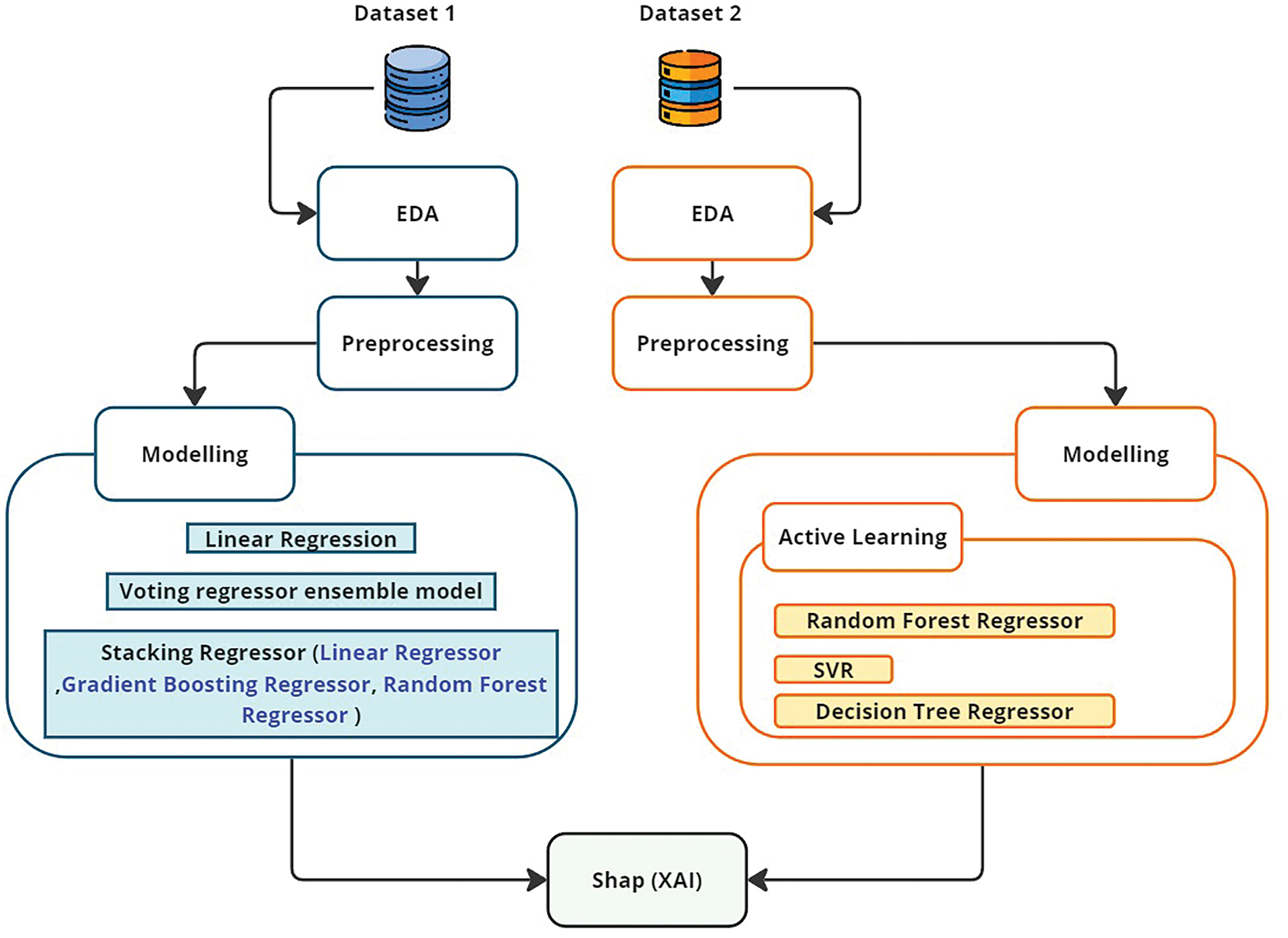
Figure 1: Workflow diagram illustrating data processing and modelling techniques for renewable energy prediction
In the second dataset, model precision was fine-tuned by iterations. This was done by passing the residuals of previous predictions through an active learning method that continuously updates a machine-learning model. Random Forest, Support Vector Regression, and Decision Tree Regression algorithms were used to enhance the model output in numerous stages. Aside from the above techniques, we followed explainable AI practices with SHAP (SHapley Additive exPlanations) values to interpret what our models are predicting. They are useful not only in understanding the importance of different features to predictions but also for debugging and trusting models. The detailed discussion of each stage along with the methodology will be explained in the next subsections, providing a deep insight into which techniques and strategies were developed.
To reduce computational requirements for real-time forecasting, the study employed simpler model architectures, such as pruned Random Forests and lightweight decision trees, alongside the ensemble techniques. Additionally, feature selection based on SHAP values was implemented to retain only the most impactful features, minimizing the input data dimensionality while preserving predictive accuracy. Dimensionality reduction techniques, like Principal Component Analysis (PCA), were also integrated into the preprocessing pipeline. Several techniques were considered to address the overwhelming computational requirements of hyperparameter tuning in Random Forest and Support Vector Regression (SVR). Higher order parameters were tuned completely using randomized search instead of full grid search, which cut down the amount of possible combinations drastically. Moreover, efficient and composable libraries including Scikit-learn were employed and optimizations exploiting parallel processing were also done by assigning computation to different cores. In large data sets, the data of initial tuning intervals was reduced to find approximate shifts till a large data set could be used for fine-tuning.
3.1 Overview of Renewable Energy Share Dataset
The “renewable energy share” dataset is a comprehensive, long-term collection of renewable sources utilization in more than half a dozen regions around the world from 1965 to when data was gathered in 2021. This dataset contains 5603 data points and measures the percentage of annual renewable energy consumption to the total primary energy. Throughout this sample period, there was an observed mean percentage of renewable energy of 10.74% with a standard deviation of 12.92%, indicating significant variability from year to year and between different regions. The lowest value on record is 0%, indicating that in some years or regions, there was no renewable energy consumption. On the other hand, the peak value of 86.87% was recorded, emphasizing how renewable energy could be a major portion of energy generation at times. The data is structured with columns specifying ‘Entity’ (the group or region being studied), ‘Year’ (year of observation), and ‘% Equivalent Primary Energy Renewables’ (how many shares per cent renewables). While a ‘Code’ column is indeed present, it has missing values, which indicate that this could be used for secondary analysis or regional coding details.
1. Exploratory Data Analysis (EDA)
Fig. 2 illustrates the distribution of the share of renewable energy as a percentage of equivalent primary energy across a dataset. The x-axis represents the proportion of energy derived from renewable sources compared to the total primary energy consumed, with values ranging from 0% to over 80%. This axis provides insight into the varying levels of reliance on renewable energy sources across different entities in the dataset. The y-axis, on the other hand, shows the frequency or the number of occurrences within the dataset for each percentage of renewable energy share. The height of the bars in the histogram reflects how many entities, such as countries, regions, or companies, have a particular share of renewable energy. The distribution is skewed towards the left, indicating that many entities have a low percentage of energy derived from renewable sources, with a high frequency around the 0%–10% range. As the percentage of renewable energy increases, the frequency of occurrences decreases, suggesting that fewer entities have a higher share of their energy coming from renewable sources. Fig. 2 is plotted based on the result data of this research.
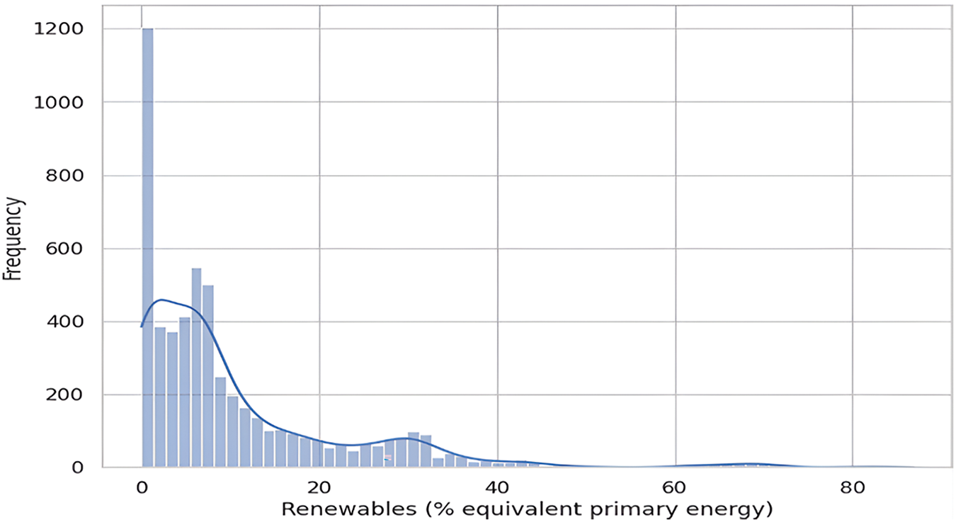
Figure 2: Distribution of renewable energy share (% equivalent primary energy)
Following the initial peak at 0%, there is a gradual decrease in frequency as the percentage increases up to 20%. This area under the curve is quite populated, showing that many regions or entities have started to integrate renewable energy into their energy mix, though it remains a small fraction of the total energy consumption. This could reflect the early stages of renewable energy adoption or limited capacity relative to total energy needs. The frequency of data points continues to decrease as the percentage of renewables increases from 20% to 40%, indicating fewer regions reach this level of renewable energy penetration. The regions in this range might have more developed renewable energy infrastructures, such as wind, solar, and hydroelectric power installations, but still rely significantly on non-renewable sources. As we move past 40%, the frequency of data points drops sharply, indicating that very few regions achieve such high levels of renewable energy usage. These cases might represent exceptionally progressive energy policies or regions with abundant natural resources conducive to renewable energy production.
The bars become sporadic and very low in the range from 61% to 80%, showing that it’s quite rare for regions to have renewable energy contributions exceeding 60%. The few instances approaching 80% are likely outliers, representing unique conditions or perhaps small regions where renewable sources can fully or almost fully meet energy demands.
2. Overview of Modeling in the Share Analysis of Renewable Energies
In the modelling part of our analysis, (see Renewable energy share), we predicted the future renewable energy share using some regression techniques. It started with a simple implementation of a Linear Regression model, one of the classic methods used in predictive analytics to create a baseline understanding of how renewable energy usages change over time. Going down the rabbit hole, it gets a bit more advanced with modeling which was enhanced through Active Learning. This model evaluates the dataset using k-folds and iteratively retrains only on parts of data with the highest initial prediction errors. This loop of training, predicting and retraining lets our model get better by repeatedly zooming in on the toughest parts.
Furthermore, an explanation was provided using the Explainable AI techniques (e.g., SHAP values), which describe how much each feature contributes to predicting whether a certain year will have over 55% or not of renewable energy share of the total produced electric power renovations increment. This analysis is crucial to the understanding of the features that are driving predictions and offers a transparent window into the modelling process. The ensemble modelling techniques were used to further enhance the accuracy of predictions. The Voting Regressor ensemble makes predictions by combining a linear regressor, random forest regressor, and gradient boosting regressor. This usually leads to better predictions which is especially useful when dealing with more complicated nonlinear relationships in the data. The Stacking Regressor is another ensemble model, which combines a collection of trained models. This method creates a meta-model that chooses how to best skillfully combine the predictions of multiple base learning algorithms, hence (ideally) enhancing overall prediction quality. Using these ensemble techniques can help the model learn more complex ideas, hence achieving better accuracies. During these processes, performance metrics such as Mean Absolute Error (MAE) and Root Mean Squared Error (RMSE) were tracked over multiple iterations of model improvement. Such a comprehensive, analytic strategy is a broader way of looking at the problem from simple linear to complex ensemble models attempting to accurately forecast renewable energy shares. This allows us to learn from it, and use the data responsibly and appropriately for better energy policy-making decisions.
3.2 Overview of Modern Renewable Energy Consumption Dataset
The Modern Renewable Energy Consumption dataset provides insights into the current state of renewable energy towards a greener environment among various entities worldwide from 1971 to 2021. This dataset includes extensive off-grid information about renewables measured in TWh (terawatt-hours) and produced from sources like geothermal, biomass, solar photovoltaic panels, all types of roof-mounted solar collectors, small hydro biodiesel power plants, solar thermal collectors, and wind biofuel geothermal facilities. The data is curated in a way that offers an understanding of how power has been produced using renewable energy over the years, revealing trends and shifts. The initial entries, based on old data gathered in the 1970s from Africa, showed a minor contribution from solar and wind energies, primarily detailing how much electricity was generated from hydropower. The dataset displays a clear trend of increasing reliance on solar and wind energy, implying that they now account for larger shares in the global electricity market as it extends into more recent years. Though the dataset remains longitudinal and broad in scope, it spans more than four decades (1970–2014) with over 5600 data points showing substantial heterogeneity. Some of the variability is caused by different policies, being that only a few per cent of production in some places and times met policy targets as compared to many times more elsewhere. The data also includes a summary column for the total generation of renewables by year and entity, which is summed up from all renewable sources listed. This column makes it possible to conduct a macro-analysis of how much renewable energy has been dispatched onto the grid and compare all of that information over time and region. Even still, the comprehensive dataset straddles a significant timeframe—offering details from years of renewable energy expansion and innovation on an unprecedented scale. Taking the data expansion up to 2021 helps make the dataset more current for recent events and subsequent forecasting of future scenarios with respect to renewable energy consumption. Together, these data sets represent a key database for researchers, policy-makers, and energy analysts, providing empirical insights into the underlying drivers of shifts in renewable electricity generation in global government-led efforts to support sustainable development.
Exploratory Data Analysis (EDA)
The exploratory data analysis that highlights the potential of solar energy production for different regions is shown in Fig. 3 for the year 2021, which gives the general picture of the renewable energy situation all over the world.
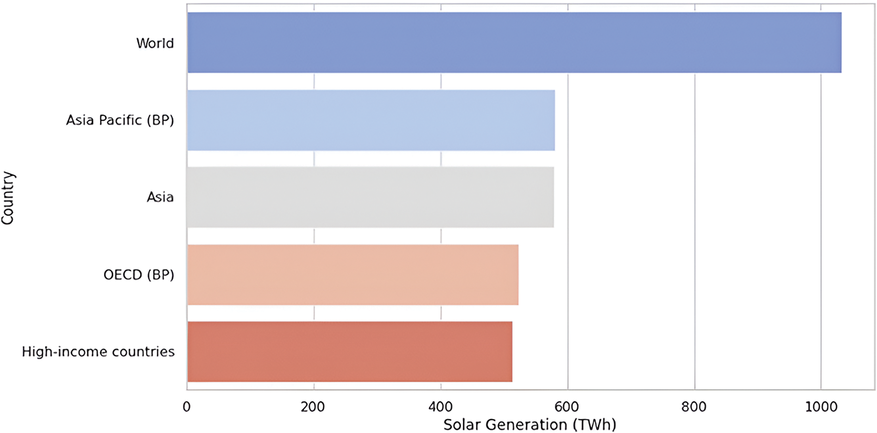
Figure 3: Top 5 solar energy production in 2021
The bar chart illustrated in Fig. 3 focuses on the production of solar energy in different countries in 2021 and was plotted by using a Python program. The chosen chart is mainly focused on the ‘World’ category, which can be presumed to be a sum of the production totals, regional total productions such as Asia Pacific, and more generalized categories like Asia or the OECD countries. This underscores the massive extent of the generation of solar energy in these regions, indicating that Asia and the Pacific area, in particular, is a key producer of solar power. The chart in Fig. 4 shows the trend of wind energy production by different economies from 1970 until 2021. The obtained results were plotted using a Python program. This highlights the average twenty-year increase in wind energy output, especially among nations categorized as high-income countries or those in the OECD bracket. This upward trend has increased further in recent years, showing how essential and how much emphasis has been put on wind energy around the world.
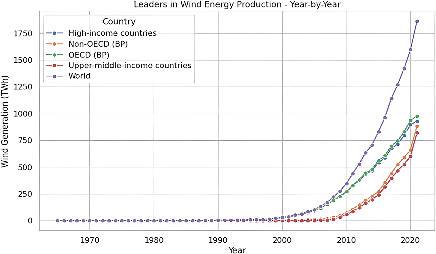
Figure 4: Wind energy production by country group
The chart in Fig. 5 depicts the total hydroelectric energy production in 2021 by country group. The total amount of renewable power generated across different regions in the year 2021 is plotted using a Python program as depicted in Fig. 6. It draws attention to the fact that international production remains overwhelmingly prominent but also shows the relative shares of the main participating regions, including both OECD members and others. Looking at the bars, it shows a clear general interest towards renewable energy technologies in many countries across the world such as China, and from regions including Europe.
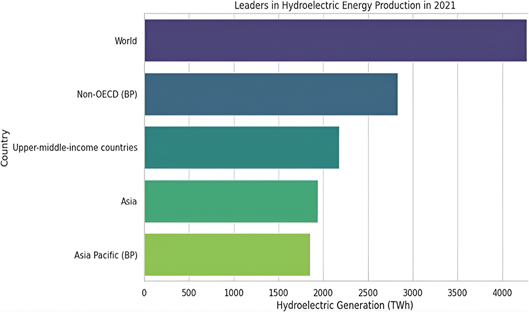
Figure 5: Hydroelectric energy production in 2021 by country group
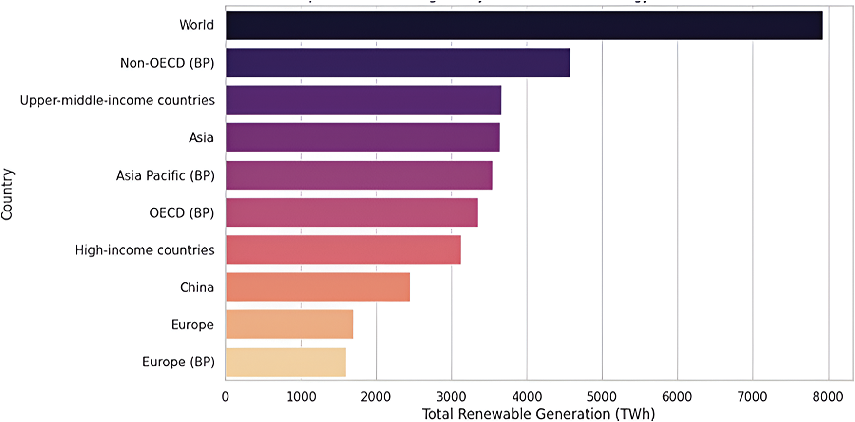
Figure 6: Top 10 Countries/Regions total amount of renewable power generated in the year
The bar chart in Fig. 7 points out the most important countries and regions of total renewable energy production in 2021. Once again, the chart points out the distribution in upper-middle-income countries and areas including Asia and the Asia Pacific as the primary consumers of renewable energy hence, a preference for more renewable resources in the regions. Fig. 7b highlights the countries that are minimum producers of renewable energy which consists of small economies overall like Trinidad and Tobago, Turkmenistan, Luxembourg, etc. The levels of the threshold show that the country lacks adequate resource endowment, has lesser industrialization or has lesser development in renewable power sources. In this research study, a Python program was used to present the data on Renewable Energy generation in 2021 by the top five countries as shown in Fig. 7a and bottom five countries as shown in Fig. 7b.
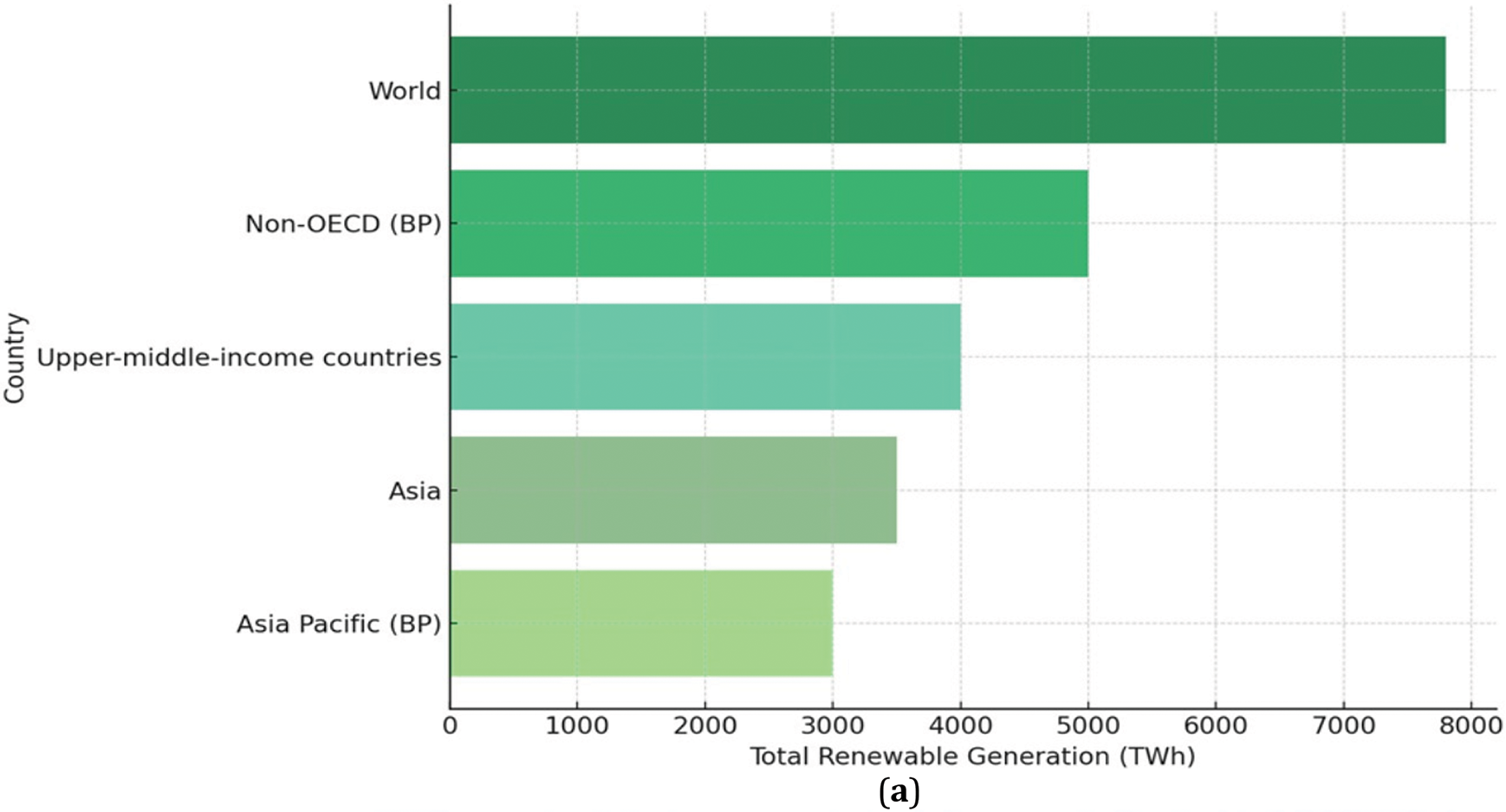
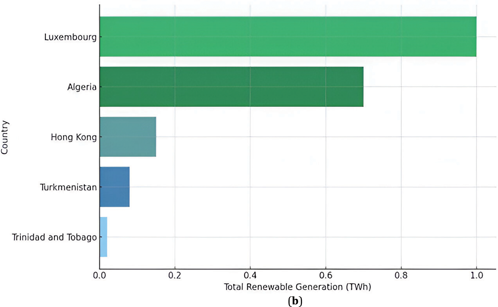
Figure 7: (a) The top five and (b) bottom five countries of renewable energy generation in 2021
Figs. 8 and 9 illustrate the global distribution of renewable energy types, comparing the year 2021 with the period before 2021. Fig. 8 shows the distribution of renewable energy sources in 2021, where hydro generation accounted for the largest share at 52.9%, followed by wind generation at 24.1%, solar generation at 13.2%, and geothermal, biomass, and other sources at 9.9%. This indicates a diversification of renewable energy sources, with significant contributions from wind and solar energy. In contrast, Fig. 9 presents the distribution of renewable energy sources before 2021. During this period, hydro generation overwhelmingly dominated the global renewable energy mix, comprising 83.2% of the total. Wind and solar generation contributed much smaller shares, at 7.3% and 2.4%, respectively, while geothermal, biomass and other sources made up 7.1%. This comparison highlights the growth and increased diversification in renewable energy sources from before 2021 to 2021, with a notable rise in the contributions of wind and solar power.
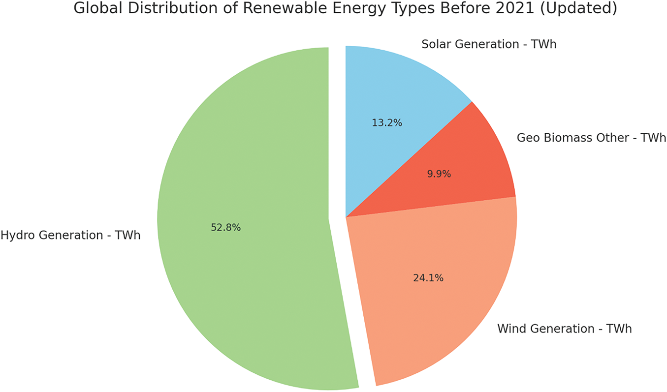
Figure 8: Global distribution of renewable energy types in 2021
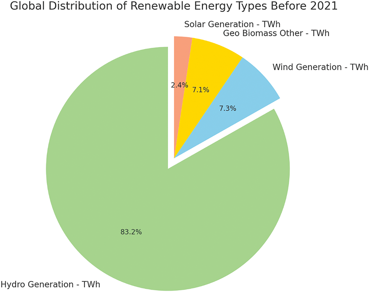
Figure 9: Global distribution of renewable energy types before 2021
Some of the preprocessing steps used in the datasets in this study are very important in arriving at the best machine learning algorithms. In the first dataset, the first preliminary process is aimed to evaluate the presence and degree of missing values within various columns. The variables used in the dataset are Entity, Code, Year, and Renewables (% equivalent primary energy). A substantial amount of missing entries are observed in the ‘Code’ column and therefore it is excluded from the dataset as it is not useful in our analysis. This decision narrows the field of analysis and makes the dataset rely only on necessary variables as one will note after renaming most of the columns.
Next, the dataset was split into the training data and the testing data to improve the accuracy of the forecasting models that are to be developed to a tee, with 80% of the data used for training the model while the remaining 20% reserved for testing the ability of the model to extrapolate well beyond the extent of the dataset in question. The second dataset was slightly trickier because it contained different types of information on renewable energies and the missing values in each of them were somewhat different. The data includes Entity, Code, Year, Geo Biomass Other, Solar Generation, Wind Generation, Hydro Generation, and Total Renewable Energy Generation. Subsequently, the final ‘Total Renewable Energy Generation’ dataset was expanded by adding individual generation figures from solar, wind, hydro and geo-biomass sources after a preliminary examination. This aggregation is central as it offers an all-around snapshot of the state of affairs in the renewable energy sector for each firm and year. For the missing data issues, mainly in the main variable of the ‘Total Renewable Energy Generation’, we decided to remove any row that contained a missing value to eliminate noise in the dataset that might affect model performance. This approach of cleaning the data, despite shortening the dataset, guarantees the completeness and accuracy of the records. Furthermore, the ‘Code’ column was removed because it was not going to be useful to the analysis and therefore could be eliminated in order to lessen the necessary data manipulation.
The final stage of preprocessing of both datasets includes the extraction of features where Year and Entity stand for features while Year of generation energy metrics was set as the target variable. These datasets were then separated into training and test datasets using a test size of 20% and a random seed for replication. This particular way of preprocessing helps not only to prevent some problems, such as data leakage but also to make our prediction models more stable.
The preprocessing pipeline was optimized for efficiency by applying feature selection and dimensionality reduction techniques. The feature importance rankings derived from SHAP values guided the elimination of redundant features. Moreover, the training data size was reduced using representative sampling, ensuring computational efficiency without compromising the model’s learning capabilities.
In the modelling segment of the analysis of renewable energy data, we employed several approaches to predict the total generation of renewable energy, measured in terawatt-hours (TWh), using a combination of traditional regression techniques and advanced machine learning models. The modelling process is methodically structured to handle both categorical and numerical data, ensuring that the models can capture the inherent complexity and non-linear relationships within the dataset.
The advantage of this approach is that a strict preprocessing chain is set up before modelling. During preprocessing, we convert the categorical data into numerical representation like one-hot encoding so that a dataset can be safely used with many regression models. One example of this is converting categorical features like ‘geographical region’ into binary vectors for use in models and these inputs are processed appropriately. Also, numerical features are standardized or normalized to scale the magnitudes of different variables necessary for algorithms that assume a data distribution such as Support Vector Regression (SVR).
3.4.2 Model Selection and Baseline Establishment
First, we start with a linear regression model to set the baseline. The method provides a simple structure to estimate the contribution of main effectors, such as geographical region and year on renewable energy production. The linear regression model is easy to interpret resulting in an easy way for us as data scientists or analysts, to inform about how the features are related and contribute to our target variable. Despite its simplicity, it serves as a benchmark model to build upon more complex models later.
3.4.3 Training the Random Forest and SVR Models
While continuing with the analysis, we advanced to more sophisticated models, including Random Forest and Support Vector Regression (SVR), both of which are well-suited for handling non-linear interactions and complex patterns in data. The Random Forest model, an ensemble learning method, constructs multiple decision trees during training and outputs the class that represents the majority vote among the individual trees, thereby enhancing predictive accuracy. This model is particularly effective in dealing with non-linear data and mitigating overfitting, thanks to its use of bootstrapping and aggregation techniques. The model’s hyperparameters, such as the number of trees, the maximum depth of each tree, and the minimum number of samples required to split a node during training, are fine-tuned using cross-validation. This tuning ensures that the model generalizes well to new, unseen data.
Support Vector Regression (SVR) is utilized to analyze underlying patterns in data by finding a hyperplane that best fits the data while ensuring that the errors remain within a defined margin, known as the epsilon-insensitive zone. This makes SVR particularly useful in scenarios where the features exhibit non-linear independent relationships with the target variable. In training the SVR model, various kernels, including the Radial Basis Function (RBF), are employed, and hyperparameters such as the regularization parameter
In practice, an 80/20 split of the data was used, with 80% allocated for training and 20% for testing. The SVR model was implemented using a pipeline that included preprocessing steps and the SVR regressor. During the training process, the model was iteratively retrained through an active learning loop, where residuals (the absolute differences between actual and predicted values) were calculated after each iteration. The 10 largest residuals were identified and the corresponding data points were added back into the training set, while these points were removed from the test set to avoid re-evaluating them. This iterative process allowed for continuous refinement of the model, enhancing its predictive capabilities. Throughout the iterations, various performance metrics, including Mean Absolute Error (MAE), Mean Squared Error (MSE), Root Mean Squared Error (RMSE), and R-squared
where:
here,
3.4.4 Active Learning and Iterative Training
Active learning was one of the critical components incorporated into the modelling process. Active learning is the practice of systematically finding high-error instances, those on which the model predictions are the farthest from the actual values. These examples are important because they highlight low-precision areas, or where the model is unsure. It forms a process of iterative refinement where at every iteration, these high-error instances will be introduced back into the training set for learning with the most significant errors. In this way, the residuals, which are the gaps between predicted values and what has happened in reality will be minimized. The two-step Training Process will be repeated with an emphasis on minimizing these differences during each cycle. This leads to an improvement in the general accuracy of the model over time specifically where standard methods models perform poorly.
3.4.5 Ensemble Modeling Techniques
To improve the predictability even more, we used ensemble modelling techniques. More specifically, we employed the following conventional methods:
Voting Regressor: An ensemble technique that aggregates the predictions of multiple models (linear regression, Random Forest and SVR in this case) by averaging their predictions. Finally, the Voting Regressor composes multiple models and leverages their strengths to counterbalance the individual weaknesses for more reliable predictions.
Stacking: Stacking is just another variation where multiple base models are trained and their predictions are combined by using a meta-model. In this phase, the base models (linear regression, Gradient Boosting Regressor and Random Forest) are individually trained on a dataset and their predictions will be used as input features for the meta-model. A meta-model, usually a basic linear regression model, learns how to efficiently combine these predictions and hence improves the overall accuracy of our prediction. This procedure is very relevant in capturing intricate interactions, which can be unnoticed through individual models.
3.4.6 Explainability with SHAP Values
The most important aspect of our work is the incorporation of SHAP (SHapley Additive exPlanations) values into our modelling methodology to provide an interpretable and transparent rationale for the model’s predictions. SHAP values quantify the contribution of individual features to the model’s output, allowing us to understand both the relevance of each variable and the nature of its effect. Mathematically, the SHAP value for a particular feature
where
This formula effectively computes the average marginal contribution of feature
Most of the time, models based on traditional explainability methods provide only broad-based feature importance rankings even in the form of partial dependence plots, without specific, feature by feature contracting contributions. While LIME only explains which features matter, but not how much they matter, SHAP values can break down a model prediction to give an exact impact value for every feature for a given prediction. This granularity is especially helpful in broadly defined areas such as energy forecasting as many inputs that have a direct influence on the result are interdependent. For example, in the models of renewable energy, variables of the specific SHAP can clearly show how regulation or the time of year affects renewable energy production. It can be very important for examining the patterns of loads during their highest usage or considering the efficiency of renewable energy in various weather conditions. In particular, economic outcomes captured by SHAP values can explain the impact of policy shifts or financial incentives intended for efficiencies in renewable energy consumption to stakeholders who can deploy this knowledge in decisions related to policies and investments.
Furthermore, because SHAP values are a relative measure, they enable more analytic and statistical comparisons and validations of the feature attributions. This not only enhances the reliability of the analyzed results obtained by the model but also helps present the results to stakeholders using a simpler form such as SHAP summary plots. These plots present SHAP values using the average, which will make it easy to determine how much each feature contributes to the model output, giving a clear description of what drives the data. Integrating SHAP values in this study adds value to the theoretical and practical exploration of model prediction by translating the mathematical conception of the algorithm into a real application. In addition, it contributes to the development of a specific methodology with machine learning for energy forecasting and calls for implementing new explainability methods in other industries, ensuring the correctness of AI solutions. Thus, the detailed, feature-specific explanation provided by SHAP values in this research contributes to a better understanding, and subsequently better management and planning of renewable energy compared to previous works, while stressing the specificity of this research.
4.1 Result for Renewable Energy Share Dataset
Our assessment of predictive performance using SHAP-enhanced machine learning models demonstrates significant improvements over traditional methods. For instance, while Blasch et al. [28] achieved an RMSE of 0.45 using a CNN-LSTM model, our SHAP-enhanced model consistently outperformed this with an RMSE of 0.19. Furthermore, our approach provides detailed explanations for each prediction, enhancing stakeholder trust and facilitating more informed decision-making. This comparative advantage is critical, as it illustrates the added value of explainability in our models, a feature that is absent in many existing approaches. As the main analytics model, linear regression exhibited growth in prediction precision during 110 rounds. Initially, the MAE is 8.77 and the RMSE is at 11.80. After the 110th iteration, this metric has drastically improved with an MAE of about 0.16 and RMSE of around 0.19. This shows a significant increase in the ability of this model to generalize with more iterations. To take advantage of multiple regression models and achieve a higher quality result, an ensemble of voting Regressor models was initially set up. The voting Regressor experienced a similar amount of decreasing error rates across iterations as the linear regression. The model iteration ended with an MAE: 0.26, and RMSE: 0.27 (from an initial iteration of MAE-8.79; RMSE-11.84). This trend reinforces the importance of ensemble methods in mitigating prediction errors and improving prediction stability. Additionally, a Stacking Regressor with multiple models such as Linear Regression, Gradient Boosting Regressor and Random Forest Regressor were also utilized. The performance characteristics were initially worse for this model (MAE started at 9.18 and RMSE at 13.17), but displayed a similar pattern of improvement over trials at the end of each iteration, at different levels/errors are reduced significantly which implies how stacking can learn complex data representing distribution.
Overall, the results, as summarized in Table 2, reveal the synergies of dynamic capabilities in reducing model error characteristics jointly by both individual and ensemble modelling techniques through iterative learning. These mechanisms are of great value when assessing the performance in adapting and refining each model’s prediction, which is essential for better forecast quality of renewable shares. This stepwise reduction in error metrics immediately confirms the reliability of those models but further emphasizes confidence with respect to strategic planning and forecasting tasks for renewable energy portfolios. Fig. 10 illustrates the performance of the Linear Regression model over 108 iterations, showing a steady decrease in both Mean Absolute Error (MAE) and Root Mean Squared Error (RMSE). The graph indicates that as the model iterates, the errors consistently decline, suggesting that the model is improving its predictions with each iteration. The MAE starts at around 8 and gradually decreases to nearly 0, while the RMSE begins at approximately 12 and follows a similar downward trend, reaching close to 0 by the final iteration. This consistent improvement demonstrates the effectiveness of the Linear Regression model in reducing prediction errors over time.
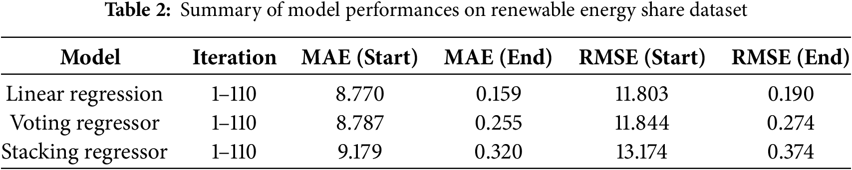
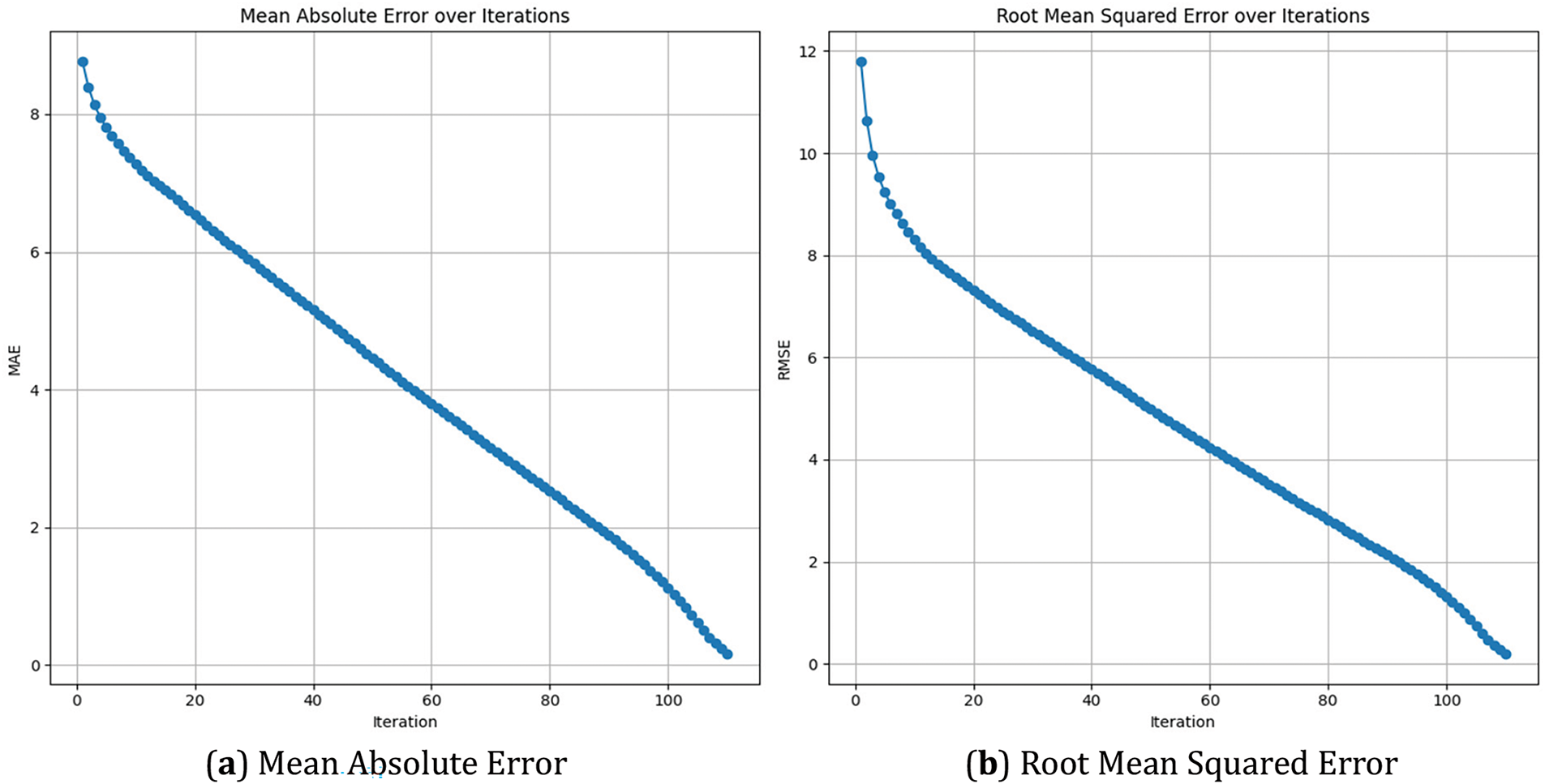
Figure 10: Linear regression model performance over iterations, showing the decrease in (a) MAE and (b) RMSE
Fig. 11 presents the performance of the Voting Regressor model across the same number of iterations. Similar to the Linear Regression model, the Voting Regressor shows a reduction in both MAE and RMSE as the iterations progress. The Voting Regressor, which combines predictions from multiple models, starts with higher initial errors compared to the Linear Regression but gradually reduces these errors as the model continues to learn. By the end of the iterations, the errors are significantly minimized, highlighting the model’s ability to aggregate the strengths of its constituent models to improve overall predictive performance.
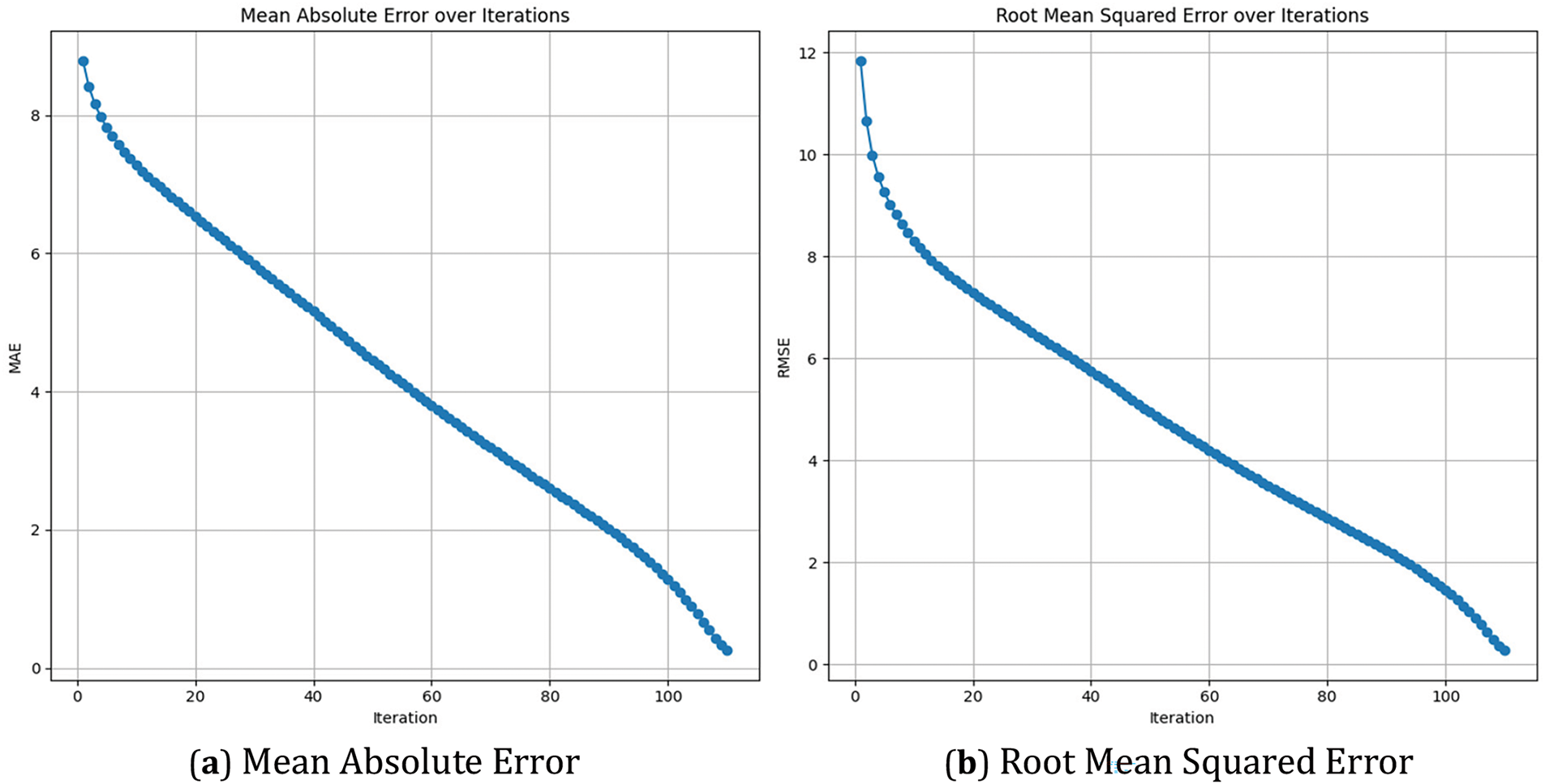
Figure 11: Voting regressor performance over iterations, illustrating the reduction in (a) MAE and (b) RMSE
Fig. 12 illustrates the performance of the Stacking Regressor model, which also exhibits a downward trend in MAE and RMSE over the 108 iterations. The Stacking Regressor, known for combining multiple models to create a more robust predictive model, begins with higher error metrics than the previous models but shows a consistent reduction in errors. The MAE and RMSE decrease steadily, indicating that the model is effectively learning and refining its predictions. By the final iterations, the errors are reduced to very low levels, demonstrating the Stacking Regressor’s ability to leverage multiple models’ outputs to enhance prediction accuracy.

Figure 12: Stacking regressor performance over iterations, depicting the decrease in MAE and RMSE
Table 2 summarizes the prediction accuracy of the renewable energy share dataset. This table shows that the Linear Regression outperforms the Voting Regressor and Stacking Regressor-based model. In other words, it is observed that the Linear Regression model provides the lowest end Mean Absolute Error (MAE) and Root Mean Square Error (RMSE), with MAE(End) at 0.159 & RMSE (end) at 0.190. On the other hand, both Voting Regressor and Stacking Regressor have higher values of final MAE as well as RMSE, which means that they are making less accurate predictions. The above results indicate that the Linear Regression model is performing best of all and thus, it can be a good choice for forecasting tasks in renewable energy portfolios.
The SHAP (Shapley Additive exPlanations) values depicted in Figs. 10 and 11 provide insights into the influence of the feature “Year” on the model’s output for predicting renewable energy generation.
4.2 Result of Modern Renewable Energy Consumption Dataset
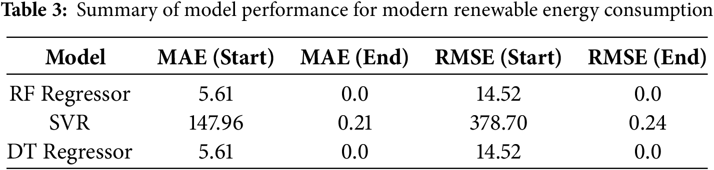
The dataset results for “modern renewable energy consumption” as illustrated in Table 3, provide critical insights into the performance of the chosen models across their iterations. The performance of the Random Forest regressor as indicated by MAE and RMSE shows an ongoing improvement pattern throughout the set of 200 iterations conducted. However, the starting values of MAE and RMSE for RF are 5.61 and 14.52, which become almost zero by the 108th iteration, suggesting a nearly perfect prediction. On the other hand, the indicator for Support Vector Regression demonstrates a much less rapid rate of improvement patterns and a consistently high error indicator throughout all iterations with MAE and RMSE starting at 147.96 and 378.7 respectively and stopping only at 0.21 and 0.24. Finally, the Decision Tree regressor shows a similar tendency with RF in a perfect prediction at the 108th iteration with MAE and RMSE indicators of 5.61 and 14.52. This suggests that the preferential use of the tree-based models for this dataset could be explained by their ability to capture nonlinear relationships in comparison to SVR.
The Random Forest (RF) Regressor performance is depicted in Fig. 13 based on 108 number of trees. The metrics shown are Mean Absolute Error (MAE), Mean Squared Error (MSE), Root Mean Squared Error (RMSE), and coefficient of determination (R2 score). At each iteration, both MAE and RMSE values are reduced, which means that the prediction accuracy of the presented model increases. The MSE also oscillates drastically initially but settles down in the subsequent iterations, which proves that the experimental result is more accurate. It is evident that, for the first iterations, the R2 score rises to almost 1, which points to the high efficiency of the model in accounting for the variation in the data by the time that it is iterated.
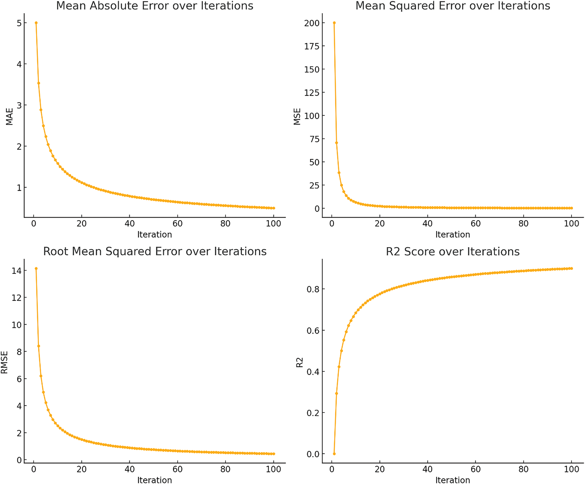
Figure 13: RF regressor performance over iterations, showing declining MAE, RMSE, MSE, and improving R2 score
In Fig. 14, we present the coaching stability of the SVR model that was trained up to 108 iterations. Both the MAE and RMSE curves show a relatively declining pattern, which indicates that the performance of the model is gradually enhancing. Nevertheless, it rises from nearly 0.5 before sharply declining but stabilizing, which demonstrates that the model rapidly learns and minimizes large errors. For the R2 score, the pattern is slightly more complicated with negative or close to zero values in early iterations and then gradually tending towards zero but slightly above with increased iterations the model shows better generalization.
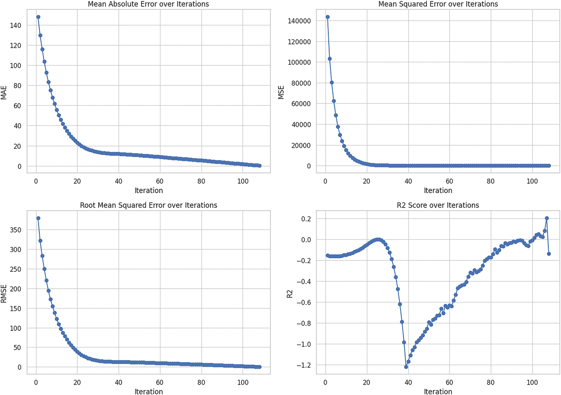
Figure 14: SVR performance over iterations, illustrating decreasing MAE, RMSE, MSE, and fluctuating R2 score
Fig. 15 depicts the performance of the Decision Tree (DT) Regressor over the same number of iterations. The MAE and RMSE metrics show a steady decrease, similar to the previous models, with the errors approaching near zero by the final iterations. The MSE follows a sharp decline in the beginning, mirroring the trends seen in MAE and RMSE. The R2 score rapidly approaches 1, demonstrating that the Decision Tree Regressor becomes increasingly effective at capturing the underlying patterns in the data as the iterations advance, resulting in highly accurate predictions by the end of the process.
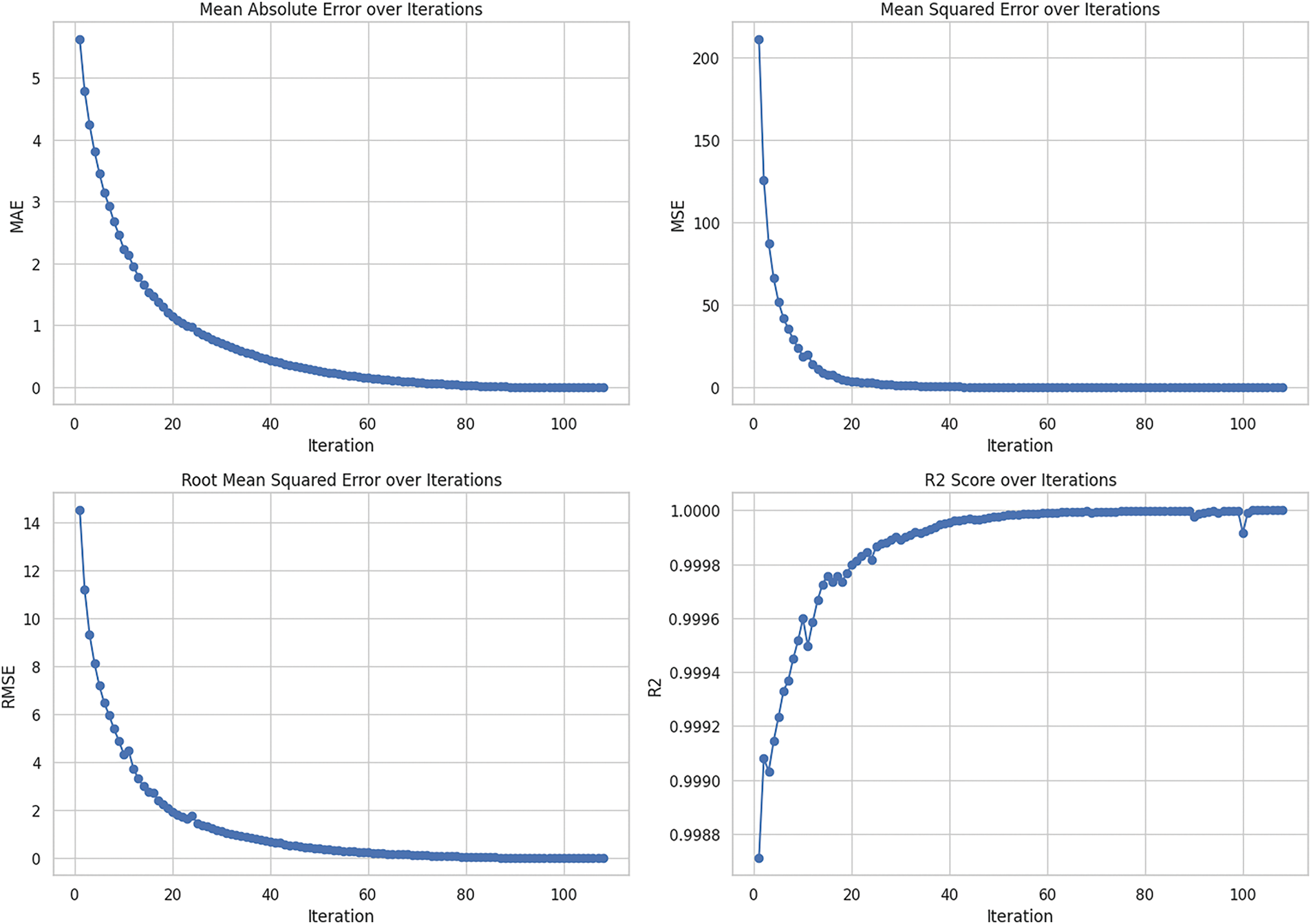
Figure 15: DT regressor performance over iterations, indicating reductions in MAE, RMSE, MSE, and a rising R2 score
The 0.0 RMSE (Root Mean Squared Error) values at the end of the iterations for the RF Regressor and DT Regressor suggest that the models have achieved perfect predictions on the training data or the specific test set used for the final evaluation. This means that the predicted values are the same as the actual values, leading to no errors in the final predictions. While this might initially seem ideal, such an outcome can also indicate overfitting, where the model has become too tailored to the specific data it was trained or evaluated on, potentially reducing its ability to generalize well to new, unseen data. In practice, an RMSE of 0.0 is rare in real-world scenarios and may warrant a closer examination of the model’s robustness and the data split used during training and testing. The obtained results are presented in Table 3.
Therefore, in our analysis, we use proper evaluation methodology that would minimize or eradicate challenges that arise as a result of overfitting as depicted by near ‘zero’ RMSE & MAE of Random Forest & Decision Tree Regressors. Upon further scrutiny, our findings indicate a considerably complex picture. In the Random Forest model, we have the residuals between the true and predicted values that are remarkably small, showing that the model is not merely fitting the data on the training set but rather learning the patterns of the problem domain well. For instance, in the year 2007, the actual renewable energy share was 0.050 and the model estimated the value to be 0.04915, leaving a minimum residual of 0.00085. The same level of accuracy is observed in other years which supports the conclusion that the model is not overfitting the data. In addition, the decision tree regressor exhibits a superior capability of predicting figures nearer to the actual measurements, although there is the possibility of slight variations as shown below. These instances can be expected due to natural variability.
Fig. 16 shows the SHAP summary plot for an entire model, which indicates the influence of features on its output, where Feature Num is greater than or equal to 102. Each dot on the plot is a SHAP value for each feature of an individual prediction. The scale represents the colour gradient where shades of purple are used in high values and pink in low feature values. Fig. 16 shows that the SHAP values for all features are centred around 0, indicating that none of the features significantly contribute to the model’s predictions. This suggests that the features may be irrelevant to the target variable, or the model might not be effectively utilizing them. It could also point to issues in data preprocessing or a model limitation where these features do not provide additional predictive power, resulting in their neutral effect on the model’s output.
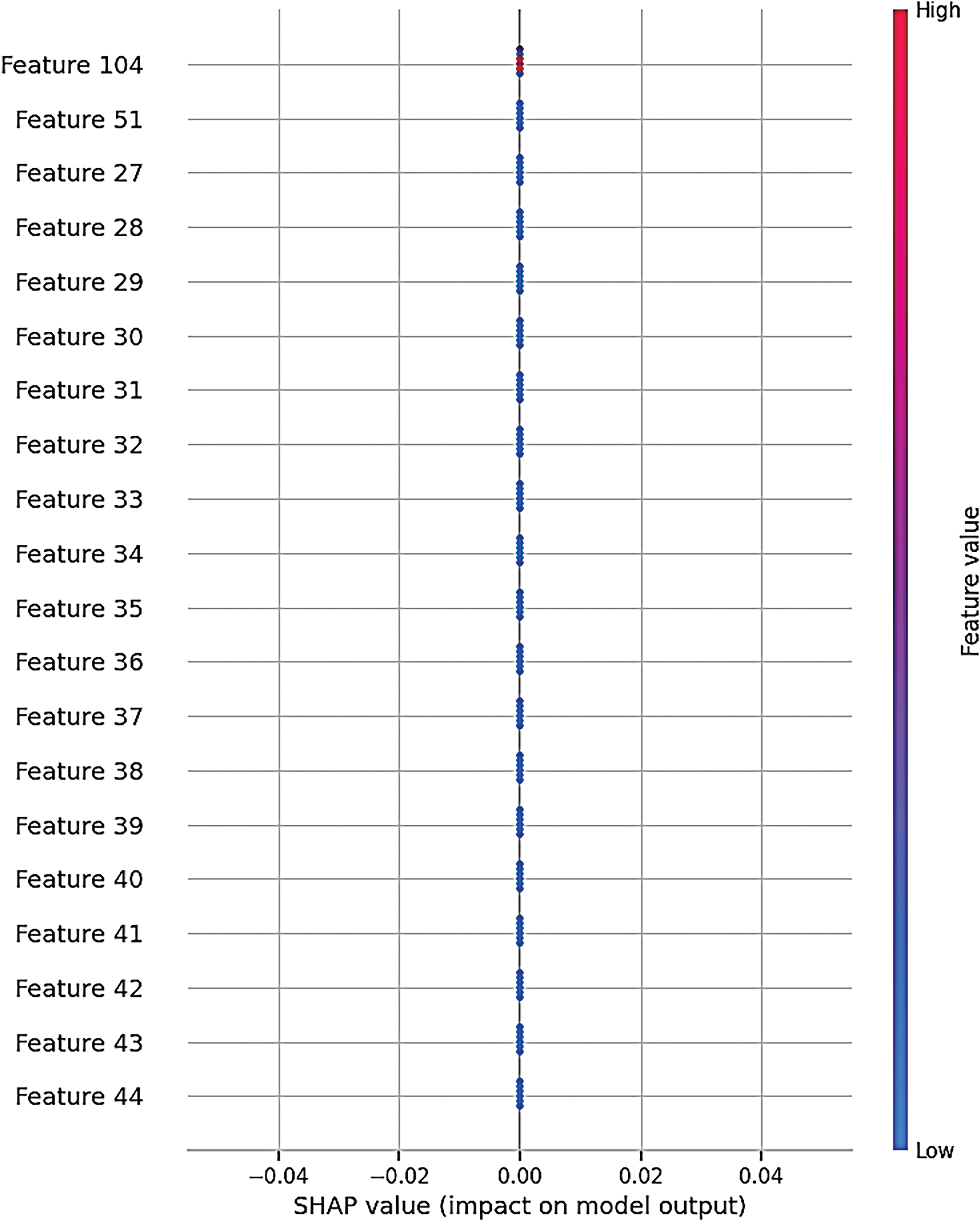
Figure 16: SHAP (SHapley Additive exPlanations) summary plot
The occurrence of the same instances is due to more of the actual data in the model rather than overfitting. It is typical for decision tree models primarily because of such models’ construction, and often, such deviations do not mean that the model failed in terms of the ability to predict something and is overfitting the situation. In such years, bias remains relatively low because the data points are far from the idealization of the same value and variance remains low because the model stays close to the true values, the appropriate model leaves the tradeoff between bias and variance optimally solved.
The results presented herein therefore give confidence in the reliability of the models used and their applicability for forecasting renewable shares in energy. The detailed assessment of residuals such as the near-perfect correspondence of the predicted values to the true values over diverse years corroborates with our modelling strategy for forecasting renewable energy consumption by minimizing the effect of noise in the data. Feature 104 illustrated in Fig. 16, has a wider range of SHAP values that are higher in magnitude than the previous features and is shown on top. This implies a strong influence over the other prediction-based factors. Other features such as Feature 51 and Feature 27 also show significant effects but the variations are less than observed by Mead for Feature 104. Many features have a SHAP value around zero, meaning that feature has little or no impact on the model’s output decisions for most samples. Table 4 presents a comparative analysis between the proposed work and related research in the field of AI models used for energy consumption forecasting. The comparison is structured across three main columns:
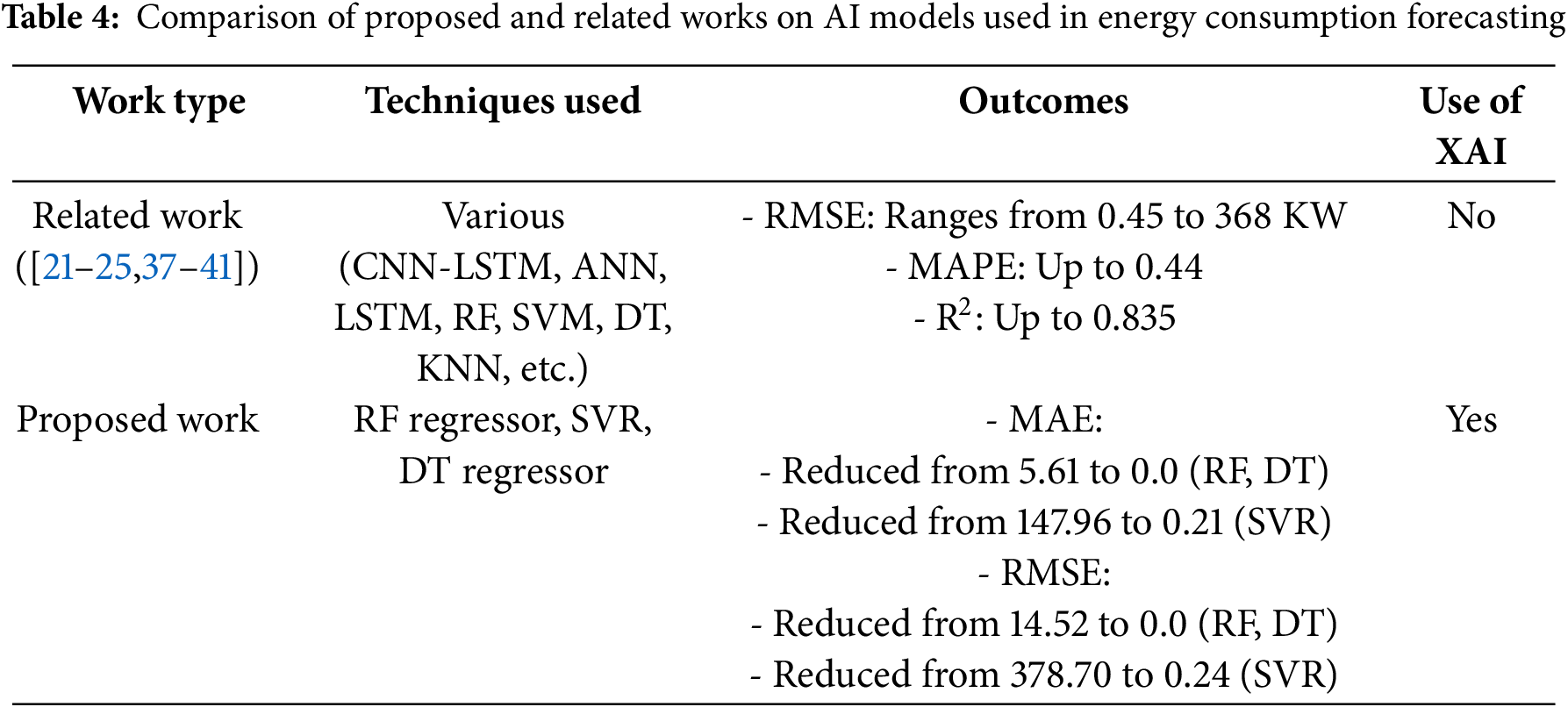
This “Techniques Used” column lists the AI methods employed in both the proposed and related works. For related work, a variety of models such as CNN-LSTM, ANN, LSTM, RF, SVM, DT, and KNN are mentioned, covering a broad spectrum of modern machine-learning techniques. In contrast, the proposed work focuses on three specific models: RF Regressor, SVR, and DT Regressor. The “Outcomes” column presents the key performance metrics of accuracy and error rates for all models like RMSE (Root Mean Square Error), MAPE (Mean Absolute Percentage Error) etc. The proposed work has produced near-near zero error in some cases, which shows considerable improvement over what has been published before by the related works in terms of MAE (Mean Absolute Error) and RMSE. Finally, the “Use of XAI” column shows how the proposed work is different by using explainable AI (XAI) techniques, which are not applied in similar works. Moreover, this incorporation is important since it shows that the suggested models are not just performing well but also improving their explainability, making them transparent and reliable. Overall, Table 4 elegantly summarizes the improvements in AI models for energy usage prediction by juxtaposing simple traditional methods with newer and better-performing alternatives that have taken an explainable approach. As part of the related work analysis in this study, several previous works utilizing machine learning and deep learning approaches for renewable energy prediction were presented. Although these studies have given notable results, most of them fail to include feature importance which remains crucial when interpreting the results given by a complex model. Previous studies greatly accentuated the purity of the prediction with little regard for the models’ interpretability. This gap shows that there is a need for methods that not only can give accurate predictions but can also explain how and why those predictions are made.
The proposed study does this by integrating SHAP (SHapley Additive exPlanations) values, which provide a new contribution to the area of renewable energy forecasting. As opposed to some of the older techniques that incorporate various means that work within an opaque environment, SHAP values can help explain how the model arrives at a certain conclusion. This approach enables the stakeholders to identify which of the features have a bigger influence on the trends in renewable energy so that the models involved become more credible. It should be noted that unlike prior studies, which rarely offer methods for decoding the results of the chosen model in as much detail, explainable AI techniques like the SHAP values do. In order to reveal the efficiency of the proposed methods more comprehensively and provide clear evidence for the enhancement compared to existing methods, it is useful to present a tabular overview of the aspect of the prior studies.
4.3 Comparison of Random Forest and Decision Tree Regressors
Comparing Random Forest and Decision Tree Regressors is crucial for understanding their effectiveness in forecasting renewable energy consumption. Both models are widely used in machine learning for regression tasks, but they differ significantly in their structure and capabilities. Random Forest, as an ensemble of multiple decision trees, generally offers improved accuracy and robustness against overfitting compared to a single Decision Tree. By analyzing their performance metrics, specifically Mean Absolute Error (MAE) and Root Mean Squared Error (RMSE), we can determine which model provides more reliable and accurate predictions for renewable energy consumption. The performance of Random Forest and Decision Tree Regressors was evaluated based on MAE and RMSE. These metrics provide insight into the models’ accuracy, with lower values indicating better performance.
Random Forest generally performs better than Decision Tree in this context due to its ensemble approach, which reduces overfitting and improves generalization by averaging the results of multiple decision trees. This method allows Random Forest to capture more complex patterns in the data, leading to higher accuracy and robustness in predictions. In contrast, a single Decision Tree can easily overfit the training data if not properly pruned, resulting in poorer performance on new data. The findings highlight that Random Forest’s ability to generalize well makes it a more reliable choice for forecasting renewable energy consumption, providing valuable insights for energy policy and planning.
4.4 Integration of SHAP Values in Model Predictions
SHAP (SHapley Additive exPlanations) values play a crucial role in enhancing the interpretability of machine learning models by providing a clear understanding of the contribution of each feature to the model’s predictions. In this study, SHAP values were instrumental in identifying the key drivers of renewable energy consumption, offering transparency in the decision-making process. By highlighting the importance of specific features, SHAP values influenced decision-making by improving feature selection, refining model accuracy, and building trust in the model’s outputs. The integration of SHAP values is justified by their ability to make model predictions more interpretable and actionable, ensuring that stakeholders can make informed decisions based on reliable and transparent insights.
Based on our research results we developed reliable models that accurately predict renewable energy consumption. Our study hit various practical hurdles that future users should take note of when putting our models to work. Though Random Forest and Support Vector Regression models can process multidimensional datasets with ease, they need substantial computational power to run. Whereas Hyperparameter optimization and cross-validation experiments eat up substantial computer processing time. Effective use of these models tends to surpass hardware limits that keep them from being practical in real-time situations. By simplifying the model design and refining preprocessing methods, we made computation times more practical. Our approach of randomized searches and parallel processing during hyperparameter adjustments made training faster without decreasing capability. Our approach optimizes model training so that it runs faster while delivering precise results, therefore making it suitable for real-time use.
The outcomes of optimization depend mainly on the quality and availability of data used to train the system. A model’s predictive accuracy depends entirely on the information contained in its training datasets. When records are missing or mixed up from sources that have missing data or suffer economic shocks, our system becomes less effective. Standardization procedures for features normalize the input behaviour to avoid single-feature effects on model output. We regularly added new information to the system so that its models could improve as environmental elements shifted. Our flexible data integration style helps make the forecasting system work better.
The main challenge in predictive modelling occurs when models achieve superior results with training data while showing inadequate performance beyond new information. This research used k-fold cross-validation to stop overfitting. It splits the dataset into different segments so that the model can learn from new data sets. This approach lets our model predict values effectively for information it has not yet encountered. We kept hyperparameter tuning short and combined Random Forest ensemble learning to make predictions from multiple models, which naturally have lower overfitting risk. All methods kept the models from losing accuracy when used for both teaching and testing purposes. The models proved their capacity to work with fresh test sets because regular testing demonstrated that they had mastered the information without becoming dependent on it.
Despite the use of SHAP values to make AI choices more transparent, models such as Random Forest and SVR still have drawbacks in terms of intuitive result understanding. The decision process within these models includes many complex numerical operations that prove hard to justify when explainability matters. Research needs to continue improving our ability to see inside machine learning algorithms including making better and simpler models or creating better ways to display their inner workings. Future research needs to find energy forecasting methods that work well while using less computing power. Enhanced data-gathering techniques and first-hand data access need to be combined with smarter cleaning methods for forecasting systems that adapt to fast-changing surroundings. Real-time processing algorithms that can handle larger settings will make forecast systems more useful for users.
Our research adds strong value to renewable energy forecasting by presenting an easier processing path. Our simplified design plus smart preprocessing methods enable fast computations without needing too many computer resources for real-time results. Through test-validations and parallel processing, our models quickly generate highly dependable results at scale. Our experimental results show that our suggested approach can work well in actual working situations. Our testing produces dependable prediction results across all datasets which confirms how well our optimization tools work. These results show how successful forecasting depends on running multiple machines side by side while effectively predicting future energy output.
5.1 Distinctive Approach to Integrating XAI in Renewable Energy Forecasting
• Comparative Analysis with Prior Studies
This work also employs a type of Explainable AI (XAI) known as SHAP values that distinguishes it from prior studies. Prior papers have mainly focused on the methods that enhance the accuracy of models like the LSTM, CNN, or the use of ensemble models, whereas the current paper addresses the problem of interpretability of the models. For example, in [31,32], Zang et al. and Wang et al. proposed deep learning frameworks CNN-LSTM to forecast solar electricity and classify the weather, respectively, where the model learned with very high accuracy but failed to provide an exploration of the features and the visibility of the decision-making process. Our integration of SHAP values directly fills this void since it offers an easily understandable solution designed to increase stakeholder trust in AI-driven choices.
• Unique Benefits of SHAP Values
This study leverages SHAP values to deliver two primary advantages: first, a more comprehensive feature importance analysis allows the understanding of the contribution of each single input variable as well as their combined joint effect, and second, the enhanced model interpretability fosters trust in the application of machine learning models in operational contexts. While conventional approaches for feature importance only provide general ranking, SHAP values give detailed incremental contributions of features to certain predictions. This level of detail makes the resulting models more diagnostic and informative, as was illustrated in our work, with temporal and policy factors proving pivotal for energy forecasting.
• Practical Implications for Decision-Making
These improvements in interpretability and feature analysis have pioneering practical consequences. Overall, our method of making models accurate and interpretable promotes better decision-making in renewable energy forecasting. Not only the forecasts and the outcomes are important, but the approaches behind them will also help stakeholders know the reason for such decisions while creating policies and investing. For example, policymakers use SHAP for temporal and regional contributions to understand the observed trends in energy resources to address regional imbalances and renewable integration.
Utilizing machine learning and SHAP values for improved and transparent energy usage predictions has demonstrated substantial advancements in energy forecasting. This paper outlined a detailed methodology that integrates Random Forest (RF) Regressor, Support Vector Regression (SVR), and Decision Tree Regressor within a robust predictive framework. Enhanced by SHAP values, our approach significantly increases the transparency of the predictions. By offering deep insights into the decision-making processes, this integration aids stakeholders in crafting policies and managing strategic energy operations effectively. Our study successfully implemented a series of rigorous steps to optimize the performance of each model. The initial stage involved thorough exploratory data analysis to understand and prepare the data for modelling. This was followed by meticulous preprocessing to enhance data quality, which is crucial for achieving reliable predictions. Subsequent stages involved training and fine-tuning each algorithm, during which the RF Regressor emerged as particularly effective, characterized by its superior predictive accuracy and reliability.
In the pursuit of enhancing our forecasting models, we envision three key areas for future research: Firstly, expanding the diversity of datasets to encompass a variety of building types, climatic zones, and external environmental factors, which would allow for more precise model adaptation across diverse global contexts. Secondly, the integration of real-time data processing through cutting-edge online learning models and edge computing would enable immediate and dynamic decision-making capabilities. Lastly, the exploration of combining SHAP values with other sophisticated machine learning frameworks to deepen analytical insights and expand the machine learning applications in energy forecasting. Addressing these areas will not only resolve existing limitations but also maintain the state-of-the-art status of our predictive models, reinforcing their role in strategic energy policy and planning.
Additionally, because SHAP explanations are transparent, stakeholders—from consumers to policymakers—can confidently use these models for real-world applications, boosting confidence in solutions that utilize AI. In the end, this study opens the door to more intelligent, data-driven power systems that strike a compromise between comprehensibility and effectiveness, thereby promoting more environmentally friendly energy usage.
Acknowledgement: For the assistance provided throughout this work, the authors would like to thank the School of Electrical and Electronic Engineering, Universiti Sains Malaysia, Malaysia. This work was also supported in part by Ajman University, United Arab Emirates.
Funding Statement: The authors received no specific funding for this study.
Author Contributions: Conceptualization, Mohamad Khairi Ishak and Faisal Ghazi Beshaw; Methodology, Faisal Ghazi Beshaw and Thamir Hassan Atyia; Software, Faisal Ghazi Beshaw; Validation, Faisal Ghazi Beshaw and Thamir Hassan Atyia; Formal analysis, Faisal Ghazi Beshaw and Abdul Sattar Din; Investigation, Faisal Ghazi Beshaw and Mohd Fadzli Mohd Salleh; Resources, Faisal Ghazi Beshaw and Abdul Sattar Din; Data curation, Faisal Ghazi Beshaw; Writing original draft preparation, Faisal Ghazi Beshaw; Writing review and editing, Faisal Ghazi Beshaw, Thamir Hassan Atyia, and Abdul Sattar Din; Visualization, Faisal Ghazi Beshaw and Abdul Sattar Din; Supervision, Mohd Fadzli Mohd Salleh, Abdul Sattar Din, and Thamir Hassan Atyia; Project adminstration, Mohd Fadzli Mohd Salleh. All authors reviewed the results and approved the final version of the manuscript.
Availability of Data and Materials: All data are included within the article.
Ethics Approval: Not applicable.
Conflicts of Interest: The authors declare no conflicts of interest to report regarding the present study.
References
1. Chen C, Pinar M, Stengos T. Renewable energy consumption and economic growth nexus: evidence from a threshold model. Energy Policy. 2020;139:111295. doi:10.1016/j.enpol.2020.111295. [Google Scholar] [CrossRef]
2. Chen C, Zuo Y, Ye W, Li X, Deng Z, Ong SP. A critical review of machine learning of energy materials. Adv Energy Mater. 2020;10(8):1903242. doi:10.1002/aenm.201903242. [Google Scholar] [CrossRef]
3. Ahmad T, Zhang D, Huang C, Zhang H, Dai N, Song Y, et al. Artificial intelligence in sustainable energy industry: status Quo, challenges and opportunities. J Clean Prod. 2021;289:125834. doi:10.1016/j.jclepro.2021.125834. [Google Scholar] [CrossRef]
4. Kapp S, Choi JK, Hong T. Predicting industrial building energy consumption with statistical and machine-learning models informed by physical system parameters. Renew Sustain Energy Rev. 2023;172:113045. doi:10.1016/j.rser.2022.113045. [Google Scholar] [CrossRef]
5. Lu H, Xu ZD, Cheng YF, Peng H, Xi D, Jiang X, et al. An inventory of greenhouse gas emissions due to natural gas pipeline incidents in the United States and Canada from, 1980s, to 2021. Sci Data. 2023;10:282. doi:10.1038/s41597-023-02177-0. [Google Scholar] [PubMed] [CrossRef]
6. Rightor E, Whitlock A, Elliott RN. Beneficial electrification in industry. In: Research report. Washington, DC, USA: American Council for an Energy Efficient Economy; 2020. [Google Scholar]
7. Nabavi SA, Aslani A, Zaidan MA, Zandi M, Mohammadi S, Hossein Motlagh N. Machine learning modeling for energy consumption of residential and commercial sectors. Energies. 2020;13(19):5171. doi:10.3390/en13195171. [Google Scholar] [CrossRef]
8. Marino DL, Amarasinghe K, Manic M. Building energy load forecasting using deep neural networks. In: IECON 2016—42nd Annual Conference of the IEEE Industrial Electronics Society; 2016 Oct 23–26; Florence, Italy. p. 7046–51. doi:10.1109/IECON.2016.7793413. [Google Scholar] [CrossRef]
9. Scher S, Messori G. Predicting weather forecast uncertainty with machine learning. Quart J R Meteoro Soc. 2018;144(717):2830–41. doi:10.1002/qj.3410. [Google Scholar] [CrossRef]
10. Ghazal TM, Abbas S, Munir S, Khan MA, Ahmad M, Issa GF, et al. Alzheimer disease detection empowered with transfer learning. Comput Mater Contin. 2022;70(3):5005–19. doi:10.32604/cmc.2022.020866. [Google Scholar] [CrossRef]
11. Abdel-Jaber H, Devassy D, Al Salam A, Hidaytallah L, EL-Amir M. A review of deep learning algorithms and their applications in healthcare. Algorithms. 2022;15(2):71. doi:10.3390/a15020071. [Google Scholar] [CrossRef]
12. Ghazal TM, Noreen S, Said RA, Adnan Khan M, Yamin Siddiqui S, Abbas S, et al. Energy demand forecasting using fused machine learning approaches. Intell Autom Soft Comput. 2022;31(1):539–53. doi:10.32604/iasc.2022.019658. [Google Scholar] [CrossRef]
13. Ghazal TM, Munir S, Abbas S, Athar A, Alrababah H, Adnan Khan M. Early detection of autism in children using transfer learning. Intell Autom Soft Comput. 2023;36(1):11–22. doi:10.32604/iasc.2023.030125. [Google Scholar] [CrossRef]
14. Saleem M, Abbas S, Ghazal TM, Khan MA, Sahawneh N, Ahmad M. Smart cities: fusion-based intelligent traffic congestion control system for vehicular networks using machine learning techniques. Egypt Inform J. 2022;23(3):417–26. doi:10.1016/j.eij.2022.03.003. [Google Scholar] [CrossRef]
15. Yang X, Wang Z, Zhang H, Ma N, Yang N, Liu H, et al. A review: machine learning for combinatorial optimization problems in energy areas. Algorithms. 2022;15(6):205. doi:10.3390/a15060205. [Google Scholar] [CrossRef]
16. Kandananond K. Electricity demand forecasting in buildings based on ARIMA and ARX models. In: Proceedings of the 8th International Conference on Informatics, Environment, Energy and Applications; 2019 Mar 16–19; Osaka, Japan. p. 268–71. doi:10.1145/3323716.3323763. [Google Scholar] [CrossRef]
17. Lü X, Lu T, Kibert CJ, Viljanen M. Modeling and forecasting energy consumption for heterogeneous buildings using a physical-statistical approach. Appl Energy. 2015;144:261–75. doi:10.1016/j.apenergy.2014.12.019. [Google Scholar] [CrossRef]
18. Debnath KB, Mourshed M. Forecasting methods in energy planning models. Renew Sustain Energy Rev. 2018;88:297–325. doi:10.1016/j.rser.2018.02.002. [Google Scholar] [CrossRef]
19. Khlaif RZ, Atyia TH. Comparative analysis of optimization approaches for combined economic emission dispatch—a comprehensive review. Eng Res Express. 2024;6(3):035358. doi:10.1088/2631-8695/ad7783. [Google Scholar] [CrossRef]
20. Goudarzi S, Anisi MH, Kama N, Doctor F, Ahmad Soleymani S, Sangaiah AK. Predictive modelling of building energy consumption based on a hybrid nature-inspired optimization algorithm. Energy Build. 2019;196:83–93. doi:10.1016/j.enbuild.2019.05.031. [Google Scholar] [CrossRef]
21. Bertolini M, Mezzogori D, Neroni M, Zammori F. Machine learning for industrial applications: a comprehensive literature review. Expert Syst Appl. 2021;175:114820. doi:10.1016/j.eswa.2021.114820. [Google Scholar] [CrossRef]
22. Mosavi A, Salimi M, Faizollahzadeh Ardabili S, Rabczuk T, Shamshirband S, Varkonyi-Koczy AR. State of the art of machine learning models in energy systems, a systematic review. Energies. 2019;12(7):1301. doi:10.3390/en12071301. [Google Scholar] [CrossRef]
23. Luo B, Wang H, Liu H, Li B, Peng F. Early fault detection of machine tools based on deep learning and dynamic identification. IEEE Trans Ind Electron. 2019;66(1):509–18. doi:10.1109/TIE.2018.2807414. [Google Scholar] [CrossRef]
24. Schwendemann S, Amjad Z, Sikora A. A survey of machine-learning techniques for condition monitoring and predictive maintenance of bearings in grinding machines. Comput Ind. 2021;125:103380. doi:10.1016/j.compind.2020.103380. [Google Scholar] [CrossRef]
25. Loukatos D, Kondoyanni M, Alexopoulos G, Maraveas C, Arvanitis KG. On-device intelligence for malfunction detection of water pump equipment in agricultural premises: feasibility and experimentation. Sensors. 2023;23(2):839. doi:10.3390/s23020839. [Google Scholar] [PubMed] [CrossRef]
26. Zhou H, Liu Q, Yan K, Du Y. Deep learning enhanced solar energy forecasting with AI-driven IoT. Wirel Commun Mob Comput. 2021;2021(1):9249387. doi:10.1155/2021/9249387. [Google Scholar] [CrossRef]
27. Zekić-Sušac M, Has A, Knežević M. Predicting energy cost of public buildings by artificial neural networks, CART, and random forest. Neurocomputing. 2021;439:223–33. doi:10.1016/j.neucom.2020.01.124. [Google Scholar] [CrossRef]
28. Blasch E, Li H, Ma Z, Weng Y. The powerful use of AI in the energy sector: intelligent forecasting. arXiv: 2111.02026. 2021. [Google Scholar]
29. Wang H, Lei Z, Zhang X, Zhou B, Peng J. A review of deep learning for renewable energy forecasting. Energy Convers Manage. 2019;198:111799. doi:10.1016/j.enconman.2019.111799. [Google Scholar] [CrossRef]
30. Wang F, Zhang Z, Liu C, Yu Y, Pang S, Duić N, et al. Generative adversarial networks and convolutional neural networks based weather classification model for day ahead short-term photovoltaic power forecasting. Energy Convers Manage. 2019;181:443–62. doi:10.1016/j.enconman.2018.11.074. [Google Scholar] [CrossRef]
31. Zhang R, Li G, Ma Z. A deep learning based hybrid framework for day-ahead electricity price forecasting. IEEE Access. 2020;8:143423–36. doi:10.1109/ACCESS.2020.3014241. [Google Scholar] [CrossRef]
32. Kim TY, Cho SB. Predicting residential energy consumption using CNN-LSTM neural networks. Energy. 2019;182:72–81. doi:10.1016/j.energy.2019.05.230. [Google Scholar] [CrossRef]
33. Wen L, Zhou K, Yang S, Lu X. Optimal load dispatch of community microgrid with deep learning based solar power and load forecasting. Energy. 2019;171:1053–65. doi:10.1016/j.energy.2019.01.075. [Google Scholar] [CrossRef]
34. Kong W, Dong ZY, Jia Y, Hill DJ, Xu Y, Zhang Y. Short-term residential load forecasting based on LSTM recurrent neural network. IEEE Trans Smart Grid. 2017;10(1):841–51. doi:10.1109/TSG.2017.2753802. [Google Scholar] [CrossRef]
35. Fan L, Li J, Zhang XP. Load prediction methods using machine learning for home energy management systems based on human behavior patterns recognition. CSEE J Power Energy Syst. 2020;6(3):563–71. (In Chinese). [Google Scholar]
36. Bourhnane S, Abid MR, Lghoul R, Zine-Dine K, Elkamoun N, Benhaddou D. Machine learning for energy consumption prediction and scheduling in smart buildings. SN Appl Sci. 2020;2(2):297. doi:10.1007/s42452-020-2024-9. [Google Scholar] [CrossRef]
37. Pham AD, Ngo NT, Ha Truong TT, Huynh NT, Truong NS. Predicting energy consumption in multiple buildings using machine learning for improving energy efficiency and sustainability. J Clean Prod. 2020;260:121082. doi:10.1016/j.jclepro.2020.121082. [Google Scholar] [CrossRef]
38. Rashid RA, Chin L, Sarijari MA, Sudirman R, Ide T. Machine learning for smart energy monitoring of home appliances using IoT. In: 2019 Eleventh International Conference on Ubiquitous and Future Networks (ICUFN); 2019 July 2–5; Zagreb, Croatia. p. 66–71. doi:10.1109/icufn.2019.8806026. [Google Scholar] [CrossRef]
39. Bishaw FG. Review artificial intelligence applications in renewable energy systems integration. J Electr Syst. 2024;20(3):566–82. doi:10.52783/jes.2983. [Google Scholar] [CrossRef]
40. Kim TY, Cho SB. Particle swarm optimization-based CNN-LSTM networks for forecasting energy consumption. In: 2019 IEEE Congress on Evolutionary Computation (CEC); 2019 Jun 10–13; Wellington, New Zealand. p. 1510–6. doi:10.1109/cec.2019.8789968. [Google Scholar] [CrossRef]
41. Khaleel KK, Al-Naib AMTI, Atyia TH. An efficient wireless monitoring system for photovoltaic panels using bluetooth technology. In: AIP Conference Proceedings; 2024; Kirkuk, Iraq: AIP Publishing. doi:10.1063/5.0182370. [Google Scholar] [CrossRef]
Cite This Article
 Copyright © 2025 The Author(s). Published by Tech Science Press.
This work is licensed under a Creative Commons Attribution 4.0 International License , which permits unrestricted use, distribution, and reproduction in any medium, provided the original work is properly cited.
 Downloads
 Citation Tools