End-to-End Audio Pattern Recognition Network for Overcoming Feature Limitations in Human-Machine Interaction

1  Introduction

In recent years, Audio Pattern Recognition (APR) has drawn growing attention from researchers, finding widespread applications in areas such as Environmental Sound Classification (ESC) [1–3], sound event detection [4,5], and Speech Emotion Recognition (SER) [6,7]. These applications span diverse scenarios including human-computer interaction, robotics, autonomous driving, and healthcare, among others. Depending on the specific task requirements, audio recognition is often formulated as a classification problem that may adopt either single-label or multi-label classification strategies. Despite the significant progress achieved in previous research on ESC and emotion analysis, several key challenges remain in practical applications. First, handcrafted features frequently fail to capture complex emotional cues. Second, raw audio waveforms inherently involve long sequential data and noise interference, making spatiotemporal information challenging to model effectively. Finally, it remains unclear how to achieve efficient fusion of dual-branch information.

In the field of ESC, researchers commonly rely on handcrafted features (e.g., MFCC, Log-Mel) combined with convolutional neural networks to identify short-time audio segments [8,9]. Beyond its importance to ESC, SER has also emerged as a research hotspot in human-computer interaction. Compared with methods that utilize invasive sensors to capture emotional signals, noninvasive, voice-based approaches are more readily applicable in real-world settings [10–12]. Furthermore, emotion recognition based on facial recognition typically requires considerable computational resources and is vulnerable to environmental factors such as lighting conditions, making real-time applications challenging. Consequently, SER has become increasingly crucial in multimodal human-computer interaction [13]. Currently, most commonly adopted solutions for ESC and SER still rely on handcrafted features such as Log-Mel [14,15]. Originally designed for automatic speech recognition (ASR), these features capture only the frequency-domain information pertinent to human auditory perception [16], and thus lack flexibility in adapting to the varying durations and spectral characteristics of different audio samples. As a result, they often struggle to fully capture the intricate semantic clues present in audio data, particularly for tasks like SER.

To address this limitation, some studies have attempted to directly utilize raw audio waveforms as model inputs and adopt multilayer network structures to learn features automatically within the model [2,17,18]. Compared to approaches based on Log-Mel or other handcrafted features, this strategy allows the feature extraction and classification steps to be jointly optimized, thereby enabling the model to learn more discriminative high-level representations. However, the relatively long duration and complex noise environments inherent to raw audio data still pose challenges such as difficulty in spatiotemporal information extraction and high computational cost [2,17,18]. Consequently, there is an urgent need to explore how techniques such as multiscale information fusion, channel attention, and aggregation strategies can be effectively integrated into end-to-end models to improve their representation and generalization capabilities in audio pattern recognition.

To tackle the aforementioned issues, we propose an end-to-end audio pattern recognition framework that emphasizes the following innovations. First, to overcome the inability of handcrafted features to capture comprehensive emotional cues in speech, we directly employ raw audio waveforms as input, seeking to enable the model to learn high-level representations that go beyond the scope of handcrafted features. Second, in light of the challenges associated with modeling raw audio waveforms, our framework adopts a dual-branch structure. On one hand, we introduce a multiscale audio context embedding module designed to more effectively extract spatiotemporal information from audio signals; on the other, we propose a global audio refinement module to capture multiscale channel and temporal cues. Lastly, we incorporate a guided aggregation module to facilitate efficient fusion of the two branches. We conduct a series of systematic experiments on multiple audio benchmarks (e.g., ESC-50, UrbanSound8K, RAVDESS and CREMA-D) to demonstrate the potential of our end-to-end approach and its performance advantages in audio pattern recognition tasks.

2  Related Work

The audio mode recognition system primarily relies on converting the raw audio signal into time-frequency representations, such as log-mel spectrograms [18] or Mel-frequency cepstral coefficients (MFCCs) [15], as input, and feeding them into deep neural networks for category prediction. This approach has been widely applied in sound event detection tasks [19]. Currently, CNN-based systems have been widely used in the APR task.

CNN-based systems typically adopt three methods. The first method uses a model with 2D convolutional layers and time-frequency representations, such as log-mel spectrograms, as the input to the first 2D convolutional layer, treating it as an image and using CNNs to achieve accurate classification. Reference [20] proposed an efficient network structure that extracts NGCC [21], MFCC, GFCC [22], LFCC [23], and BFCC [24] features from the input tensor. Reference [25] proposed an effective method for classifying environmental sound spectrograms based on CNN, using Mel spectrograms as the feature. Reference [26] proposed an environmental sound classification algorithm based on adaptive data padding by filling short raw audio data with random padding and converting the raw audio data into log-mel spectrograms.

The second method defines an end-to-end system, typically extracting Mel spectrograms as input from the raw audio or using one-dimensional convolutional layers to extract two-dimensional features instead of time-frequency representations. Reference [27] proposed a CNN system called “efficient residual audio neural network,” which improves the inference speed of APR tasks. Reference [28] integrated high-level components, including multi-head attention, residual modules, and capsule modules, which together enhance the model’s ability to capture global and local features necessary for accurate sentiment classification. Reference [2] used transfer learning strategies to design a general-purpose end-to-end audio embedding generator that can quickly adapt to various acoustic scenarios and event classification applications. Reference [29] proposed a novel end-to-end ESC system by combining the end-to-end system and log-mel CNN, which uses a CNN for classification. Both of these approaches share the following limitations: they first convert the audio signal into a time-frequency representation, which can lead to the loss of subtle temporal information present in the raw waveform. Moreover, the feature extraction process relies on empirical knowledge, requiring manual design or parameter tuning, and thus cannot fully achieve automated optimal feature learning.

To overcome the above issues, the third approach directly uses the raw audio waveform as input. Reference [2] proposes a general end-to-end audio embedding generator that operates directly on raw waveforms. Meanwhile, Reference [3] introduces an end-to-end approach based on 1D CNNs for environmental sound classification, enabling the model to learn representations directly from the audio signal. Overall, these three CNN-based methods struggle to model global features due to the constraints of local receptive fields-an issue that becomes especially pronounced when handling raw audio waveforms, where global features play a vital role in time-dependent audio classification tasks.

Transformer-based audio processing systems, which excel at learning global features, have gained popularity in APR tasks. Their outstanding performance has already permeated much of the audio processing field. For instance, Reference [30] applied a transformer to mel-spectrogram patches, achieving significant results across multiple datasets. Reference [1] designed a hierarchical audio Transformer model that reduces model size and training time while maintaining excellent performance. Considering the performance and computational trade-offs between transformers and CNNs, researchers have explored hybrid architectures that combine both. For example, Reference [17] proposed an end-to-end model using raw audio signals and employed lightweight audio data alongside novel audio augmentation strategies, exhibiting strong generalization capabilities. In References [31–33], CNNs are used to extract low-level, local features from mel-spectrograms, which are then processed by a transformer for global semantic modeling. This approach shows excellent performance in audio classification tasks and effectively addresses the shortcoming of traditional CNNs in modeling global features.

In further developments, researchers have proposed multi-branch hybrid architectures to fully exploit feature representations. These architectures process different types of features through multiple branches and employ appropriate fusion strategies to achieve performance enhancement. For instance, Reference [34] introduced a multi-branch architecture combining parallel CNN and Transformer for speech emotion recognition. This approach processes Mel spectrograms and other features separately, extracting diverse feature representations through parallel branches, which are then fused in the fully connected layer to enable efficient emotion classification. Similarly, References [35,36] designed a dual-stream CNN-Transformer network, where two branches are used to extract spatial and temporal features respectively, and the fusion module is employed to integrate the branch-specific information, further improving model performance.

In addition, multi-scale processing has shown significant progress in audio feature extraction in recent years. For example, Reference [18] dynamically adjusted the stride and kernel size of convolutions to capture both short-term and long-term dependencies in audio signals, thereby improving computational efficiency. Reference [37] utilized filters of varying sizes to process audio inputs, enabling the extraction of multi-scale features. Furthermore, Reference [38] proposed an asymmetric multi-scale convolutional kernel design, which effectively enhanced the correlation between temporal and pseudo-frequency domains while significantly reducing computational demands. However, these methods exhibit limitations in their branch designs regarding multi-scale extraction of spatiotemporal information, particularly in their inability to fully consider the differences and complementary information between branches during the fusion process.

To address these issues, we propose a bilateral CNN-transformer hybrid architecture that directly takes raw audio waveforms as input, comprising three components: a semantic branch, a detail branch, and a guided fusion module. Specifically, the semantic branch—with a narrow channel width and deep hierarchical structure—captures broad semantic information, whereas the detail branch—with a wide channel width and shallow hierarchical structure—focuses on fine-grained temporal details. The guided fusion module integrates complementary information from both branches by leveraging the contextual information in the semantic branch to guide feature responses in the detail branch, enabling more efficient communication between the two branches.

3  Methodology

This section provides a detailed exposition of our proposed bilateral end-to-end audio classification network with semantic and detail branches. The network comprises three parts: the semantic branch, the detail branch, and the guidance fusion module. We focus on introducing three key concepts: (1) The semantic branch with narrow channel sizes and deep hierarchies, capable of processing semantically broad information (2) The detail branch with wide channel sizes and shallow hierarchies capable of processing temporally detailed information (3) An effective aggregation layer is designed to fuse these two different types of representations. We demonstrate the overall architecture and specific design concepts, as illustrated in Fig. 1.

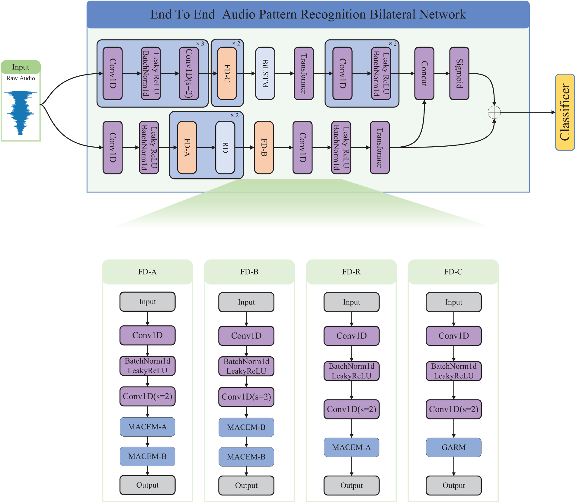
Figure 1: Overall structure of the model

3.1 Semantic Branching

Considering the balance of large receptive fields and efficient computation, this paper proposes semantic branches with multi-scale feature extraction capabilities to meet the context dependence and large receptive fields required for high-level semantics. The semantic branch mainly includes the Fast Downsampling module (FD) and the Multi-Scale Audio Context Embedding Module (MACEM). MACEM has two variants, MACEM-A and MACEM-B. For the details of these two variants, see 3.1.1.

Specifically, we design three different modules, FD-A, FD-B, and FD-R, to capture dependencies at different time scales, whose structures are shown in Fig. 1. The difference between FD-A and FD-B lies in the fact that the former uses MACEM-A and MACEM-B, while the latter uses two MACEM-Bs, and FD-R EMbeds only MACEM-A. The FD module firstly uses a one-dimensional convolution to aggregate the information, and then uses a one-dimensional convolution with a step size of 2 to reduce the size of the features and feeds them into MACEM-A and MACEM-B for a larger receptive domain to encode high-level semantic contextual information.

The original audio feature As (As ∈ R1×L, where 1 denotes the dimensionality of the feature channel and L corresponds to the feature length.) is passed through a one-dimensional convolution to increase the number of channels and improve the feature expression, and then it is passed through five consecutive FD modules to rapidly downsample the input features to obtain a larger receptive domain and encode high-level semantic context information to get the feature Asd (Asd ∈ R256×L32), and a one-dimensional convolution is used again to decrease the number of channels in order to reduce the amount of computation, and then it is inputted into the Transformer to perform the encoding, the reason for not inputting the features directly into the Transformer at the beginning is to consider that the feature size is too large and inputting it at this point would result in a huge amount of computation. The MACEM-A and MACEM-B modules of the FD module, which expand the receptive field and increase the level of feature characterization, where adaptive global average pooling and adaptive global maximum pooling are embedded into the global contextual response to further improve its performance.

3.1.1 Multi-Scale Audio Context Embedding Module

In order to reduce the loss of context information in different sub-domains, we design a plug-and-play multi-scale audio context embedding module, which contains information between different scales and sub-domains, and aggregates the speech from different regions, so that the model has the ability to understand the global context information. Its concrete implementation is described in detail below.

Combining the advantages of pyramid, we propose the multi-scale audio context embedding module (MACEM) has the form of MACEM-A and MACEM-B, as shown in Fig. 2, “⨁” represents summation operations, while “⨂” denotes element-wise multiplication. MACEM-A: Firstly, the input feature H is convolved by three one-dimensional convolutions (f1,f7,f15), whose convolution kernel sizes are 1, 7, 15, respectively, and the extracted features are concatenated from the channel dimensions in order to obtain multiple scale aggregation information, and then the number of channels is reduced to 1/3 of the original by a one-dimensional convolution f7 to obtain the feature M as shown in Eq. (1).

M=δ1(f7[δ2(f1(H));δ2(f7(H));δ2(f15(H))])(1)

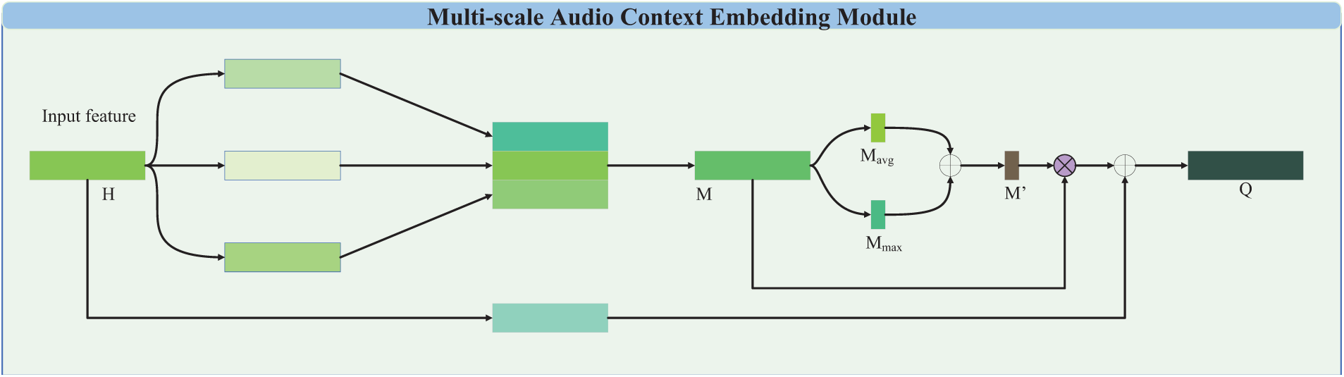
Figure 2: The structure of the multi-scale audio context embedding module

Here, we use ReLU(δ1) and LeakyReLU(δ2) activation functions to process features. H, M ∈ RC×L where C denotes the dimensionality of the feature channel and L corresponds to the feature length. The feature M is obtained by adaptive global average pooling and adaptive global maximum pooling respectively after the features Mavg and Mmax are input into two consecutive convolutional layers f, which have convolutional kernel size of 1, for compression and then the output features are summed up, and the scores for the different time and magnitude dimensions for the channels are obtained by sigmoid(σ), and M′ as shown in Eq. (2).

M′=σ(f(δ1(f(Mavg)))+f(δ1(f(Mmax))))(2)

Here M′,Mavg,Mmax ∈ RC×1 where C denotes the dimensionality of the feature channel and 1 corresponds to the feature length.

Finally M′ is multiplied with the feature M and added with the input feature H obtained by a one dimensional convolution f7 with a convolution kernel of 7 to obtain the output feature Q as shown in Eq. (3).

Q=δ2(M⨂M′+f7(H))(3)

Here Q ∈ RC×L where C denotes the dimensionality of the feature channel and L corresponds to the feature length. “⨁” denotes element-wise multiplication.

MACEM-B is to change the splicing of three one-dimensional convoluted features in MACEM-A to addition, and remove the spliced one-dimensional convolution to obtain feature M, in addition to the rest of the operation is the same as MACEM-A, MACEM-B to obtain feature M as shown in Eq. (4).

M=δ1(δ2(f1(H))+δ2(f7(H))+δ2(f15(H)))(4)

3.2 Detail Branching

The detail information and the receiving domain are key to achieving high accuracy. However, it is difficult to fulfill these two requirements simultaneously. Based on this, we propose a detail branch to preserve the detail size of the original input audio and encode the rich temporal information. The detail branch achieves 8-fold fast downsampling of the input raw audio feature As (As ∈ R1×L) by three successive layers of downsampling, each layer including a one-dimensional convolution with stride = 2, convolution kernel size 3, batch normalization [39] and LeakyReLU [40]. Then after two FD-Cs, each including a one-dimensional convolution with stride = 2, the contextual encoding of local information is performed to achieve 32-fold fast downsampling of the input raw audio features As. The final 32-fold downsampled feature Ad(Ad ∈ R256×L32) contains a large amount of detailed information, which is sequentially passed into BiLSTM (Bi-directional Long Short-Term Memory) [41] to extract the temporal information and Transfomer [42] for encoding to extract the global information. The details of the structure are given in Fig. 1. FD-C uses a Global Audio Refinement Module (GARM) to aggregate channel and temporal information at multiple scales.

3.2.1 Global Audio Refinement Module

We propose Global Audio Refinement Module (GARM) to obtain multiple scale aggregated channel and temporal information as shown in Fig. 3, “⨁” represents summation operations, while “⨂” denotes element-wise multiplication. GARM: The input feature H is convolved by three one-dimensional convolutions (f1,f3,f9), whose convolution kernel sizes are 1, 15, 15, and nulling rates are 1, 3, and 9, respectively, which are then summed up to obtain the feature K as shown in Eq. (5).

K=δ1(f(δ2(f1(H))+δ2(f3(H))+δ2(f9(H))))(5)

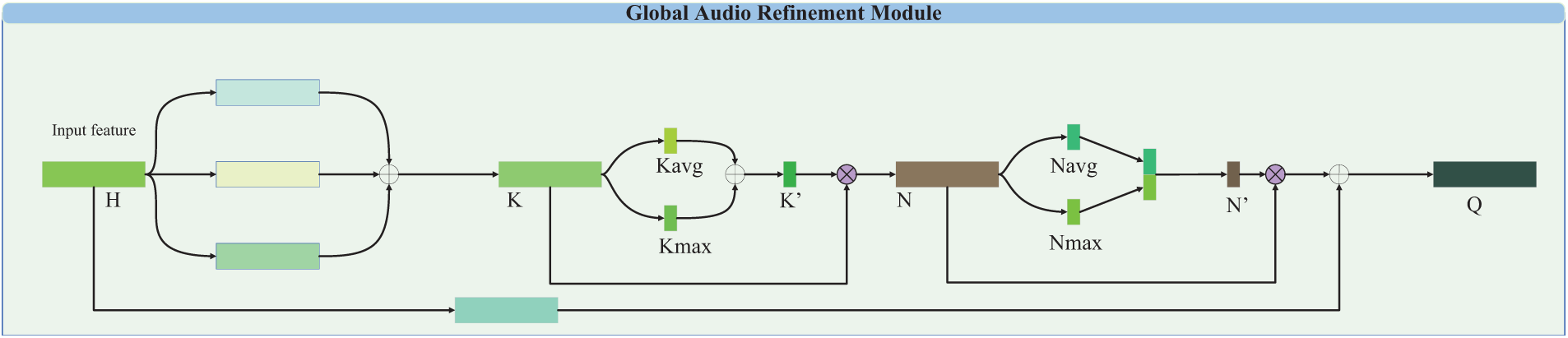
Figure 3: The structure of the global audio refinement module

The feature K is obtained by adaptive global mean pooling and adaptive global maximum pooling respectively after the features Kavg and Kmax are input into two consecutive convolutional layers f, which have convolutional kernel size of 1. Compression is performed while the output features are summed up, and the scores K′ for the different temporal and magnitude dimensions for the channel are obtained by sigmoid, as shown in Eq. (6). Finally K′ is multiplied with the feature K to obtain the feature N, as shown in Eq. (7).

K′=σ(f(δ1(f(Kavg)))+f(δ1(f(Kmax))))(6)

N=K⋅K′(7)

Feature N again through adaptive global average pooling and adaptive global maximum pooling respectively after obtaining features Navg and Nmax after inputting two consecutive convolutional layers f, which convolutional kernel size are 1, for compression and then the output features from the channel dimension after concat after a one-dimensional convolution f7 will be reduced to the number of channels to the original 1/2 to obtain the feature N′, feature N′ through sigmoid as shown in Eq. (5) to obtain the scores for the channels at different times and channel dimensions are multiplied with N, as shown in Eq. (8).

N′=σ(f7[f(δ1(f(Navg)));f(δ1(f(Nmax)))])(8)

Finally N′ is multiplied with N and summed with the input features H after a convolution kernel of 7 one dimensional convolution f7 output features to get the final output Q as shown in Eq. (9).

Q=δ2(N⋅N′+f7(H))(9)

3.3 Guided Aggregation Module

In audio classification networks, the different downsampling strategies of semantic and detail branches lead to different vector lengths and semantic gaps in the feature representations they extract. To eliminate this disparity and fuse the two types of feature representations, traditional fusion methods, such as element summation and concat, ignore the disparity between the two types of information, and thus the performance is poor and difficult to optimize. Therefore, this paper proposes a guided aggregation module to fuse complementary information from two branches to capture feature representations at different scales and to intrinsically encode multi-scale information. In addition, the guided aggregation module uses the contextual information of the semantic branch to guide the feature response of the detail branch, thus making the communication between the two branches more efficient. The experimental results in this paper show that this approach can significantly improve the performance of audio classification networks. The detail branch output feature D is adjusted by two one-dimensional convolution f to adjust the feature size to be consistent with the size of the semantic branch output feature S, and then the sigmoid function is used to obtain the score D′ for the semantic branch as shown in Eq. (10). Referring to the residual structure semantic branch output feature S is multiplied with D′ and then added with S to get the final output feature O as shown in Eq. (11). The detailed implementation and design concept is shown in Fig. 4.

D′=σ(δ2(f(δ2(f(D)))))(10)

O=S⋅D′+S(11)

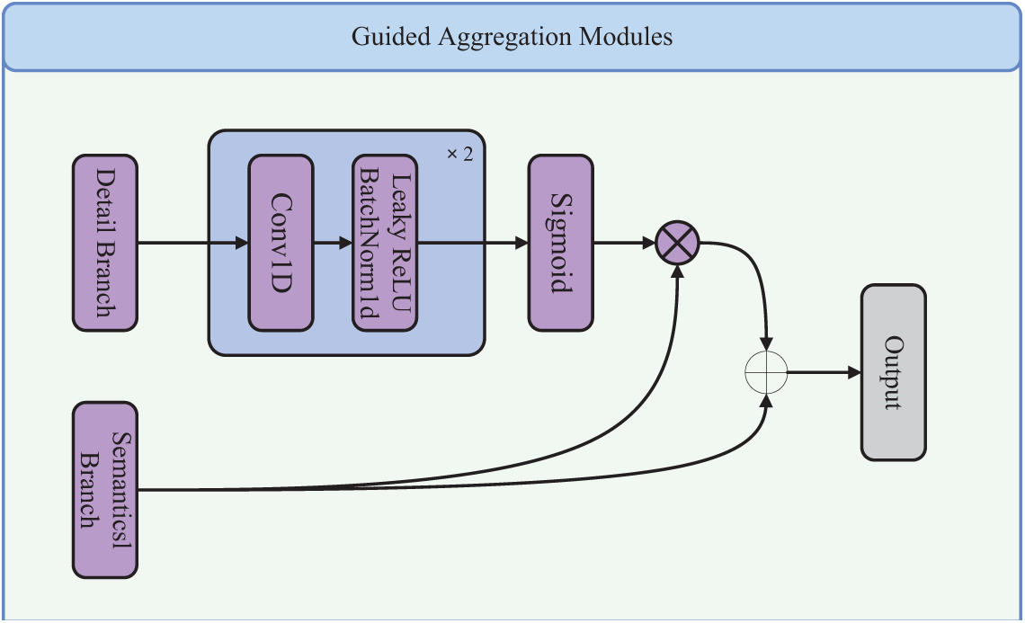
Figure 4: Guided aggregation module

Here D ∈ RC×L1, S ∈ RC×L2, D′ ∈ RC×1, O ∈ RC×L2 where C denotes the dimensionality of the feature channel and 1 corresponds to the feature length.

4  Experiment

In this section, we evaluate the effectiveness of the proposed method through experiments and compare it with existing state-of-the-art approaches. The experiments include performance evaluation on four public datasets, ablation studies on key modules of the model, and visualization analysis of the results.

4.1 Dataset Description and Implementation Details

4.1.1 Dataset Description

This section evaluates our method on public classification datasets such as ESC-50 [43] and UrbanSound8K [44]. In addition to the ESC scenario, the system was examined on the speech emotion recognition RAVDESS [45] and CREMA-D [46] dataset to show robustness to audio signal types.

The ESC-50 dataset consists of 2000 samples of ambient sounds from 50 categories. The 50 categories are animals (dogs, chickens, pigs, cows, frogs, cats, hens, flying insects, sheep, and crows), nature sounds, and water sounds (rain, waves, fire crackling, crickets, bird calls, water drops, wind, water pouring, toilet flushing, and thunderstorms). Human non-language (baby crying, sneezing, clapping, breathing, coughing, footsteps, laughter, brushing teeth, snoring, and drinking/drinking), indoor and domestic sounds (knocking, mouse clicking, keyboard typing, door, wood creaking, opening a can, washing machine, vacuum cleaner, alarm clock, clock ticking, glass breaking), and outside and urban noise (helicopters, chainsaws, sirens, car horns, engines, trains, church bells, airplanes, fireworks, and handsaws). Each sample has a length of 5 s and a sampling frequency of 44,100 Hz.

The UrbanSound8k dataset consists of 8732 audio clips, totaling 7.3 h of audio recordings. The maximum duration of the audio segment is 4 s. The raw audio sampling rate is between 16 and 48 KHz. The dataset contains 10 categories: air conditioning, car horn, kids playing, dog barking, drilling, engine idling, gunshots, jackhammers, sirens, and street music.

The RAVDESS dataset contains speech and song recordings of 247 untrained Americans categorized into 8 different levels:relaxed, happy, sad, angry, scared, disgusted, and surprised, with a neutral base for each performer. Contains 1440 files: 60 trials of 24 actors per actor, for a total of 1440 voice files.

CREMA-D is an audiovisual dataset featuring 7442 video clips from 91 actors of diverse racial and ethnic backgrounds (Asian, African American, Caucasian, and Hispanic). The actors were instructed to utter 12 sentences across six different emotions (anger, disgust, fear, happiness, neutral, and sadness) and four levels of intensity (low, medium, high, and unspecified). The average length of video clips in CREMA-D is 2.63 ± 0.53 s. We considered six emotion categories.

The dataset is divided into a training set and a test set to ensure a training and test ratio of 80:20, respectively. The sampling rate was downsampled to 22,050 Hz and short samples were zero-padded to 4 s.

In Fig. 5, we show the visualization of audio data where we selected eight audio clips from the RAVDESS dataset for processing. In this figure, eight different emotional states are represented in order from left to right, including neutral, relaxed, happy, sad, angry, scared, disgusted and surprised. And from top to bottom, different representation layers of the audio data are presented, including the original audio waveform graph, STFT-spectrogram (Short Time Fourier Transform Spectrogram), FBSP-spectrogram (Frequency Bandsplit Excitation Features), Mel-spectrogram, and MFCC (Mel Frequency Cepstrum Coefficient).

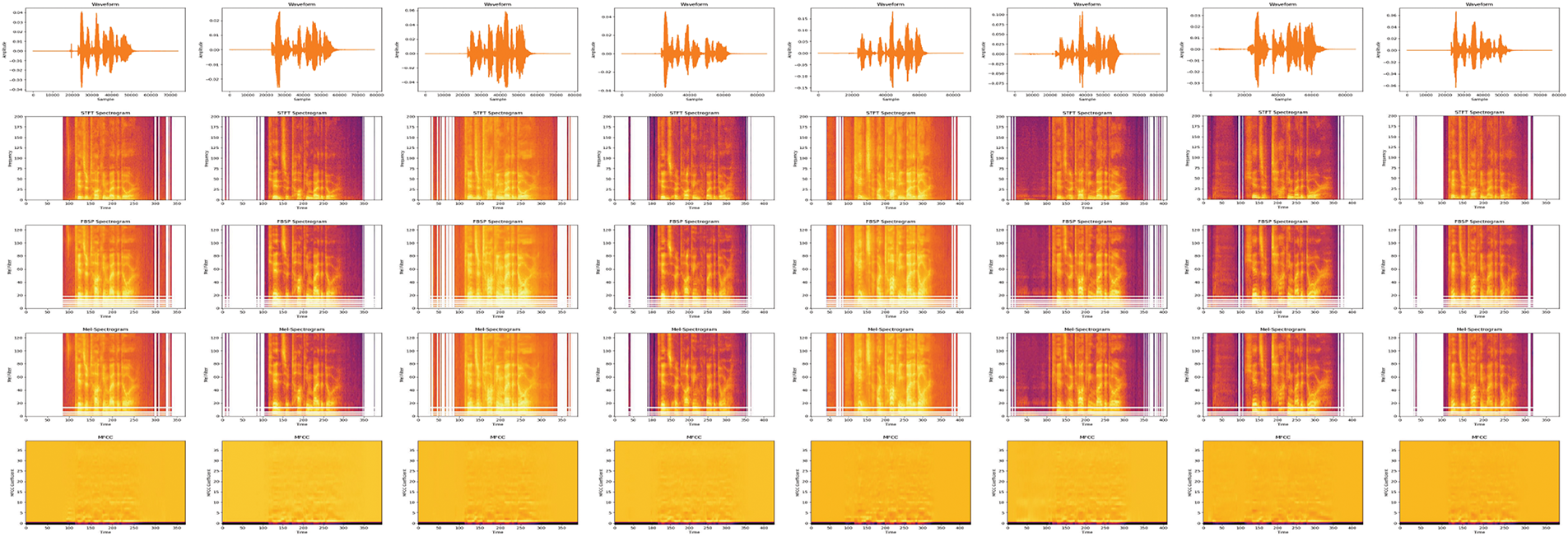
Figure 5: Audio visualization

4.1.2 Implementation Details

Our experiments are carried out on a computer equipped with Windows 11 operating system with Intel Core i9-12900KF CPU and NVIDIA RTX 3090 Ti GPU hardware configuration. The software environment is PyTorch 1.13.0 and torchaudio 0.13.0 and their dependency libraries.

For the training process, we used the AdamW [47] optimizer with a maximum learning rate of 3 × 10−4 and a one-cycle strategy [48]. In addition, we trained batches of 64 using a 10−5 decay of weights with an EMA [49,50] decay rate of 0.995, SKD of [51], and default values for all other parameters. Each of the three datasets used has an iteration of 1500. to handle the different sample lengths across the datasets, we adjusted the parameters of the samples under the control network. One noise type and one mixing strategy were randomly selected in each iteration.

As illustrated in the Fig. 6, the workflow can be divided into two primary stages: Data Processing and Training and Testing. In the data processing stage, the raw audio data is first downsampled to a sampling rate of 22 kHz, and the duration of each audio clip is standardized to 4 s to ensure compatibility with the model’s input requirements. After preprocessing, the data is split into training and testing sets. In the training and testing stage, the training data is loaded into the model for training, during which the loss function is optimized iteratively to update the model parameters and generate prediction results. The trained model is subsequently saved (as indicated by “SaveModel”) for use in the testing phase. In the testing phase, the saved model is loaded to make predictions on the testing data, yielding the final prediction results. This workflow comprehensively and systematically outlines the entire pipeline from raw data preprocessing to model training and testing, providing a clear depiction of the logical structure of our research methodology.

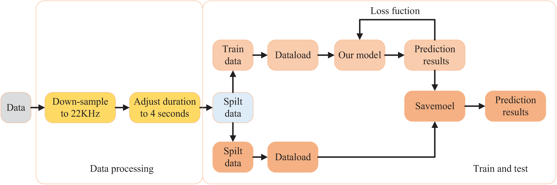
Figure 6: Schematic diagram of the overall pipeline

4.2 Results and Discussion

4.2.1 Comparison With Other Algorithms on the ESC-50

In this study, we comprehensively compare and analyze the experimental results from three different perspectives (nature of end-to-end models, form of input data, and use of pre-trained models). The experimental results are shown in Table 1. We found that the end-to-end models generally exhibit excellent performance in these aspects of the study, which is mainly attributed to their strong learning ability and robustness. Compared to non-end-to-end models, end-to-end models [2,17] show better performance in audio classification tasks.

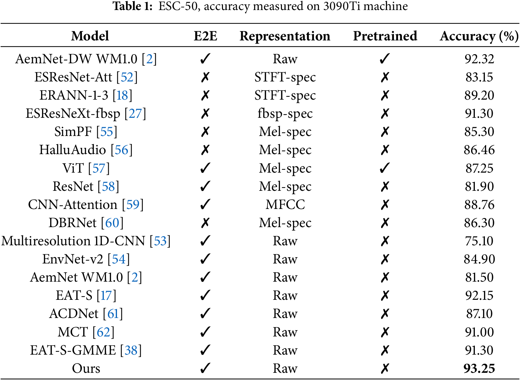
Introducing the use of a pre-trained model significantly improves the robustness of the model [2], whereas the model performance is more limited without the introduction of a pre-trained model. For the analysis of the form of input data, we observe that models using STFT-spec (short-time Fourier transform spectrum) as input data [18,27,52] outperform models using raw audio data [2,53,54] overall. STFT-spec is able to more accurately capture audio features perceived by the human ear with a certain degree of translational invariance. However, it is worth noting that the process of transforming audio into STFT-spec loses some of the detailed information of the original audio signal as well as the fact that generating STFT-spec involves the selection of some hyperparameters. This may lead to difficulties for the model to accurately distinguish different audio categories in a complex context such as human-computer interaction. To address this issue, our proposed model successfully solves this challenge. In addition, previous research [43] confirmed that using raw audio as input has great potential in audio categorization tasks. In this study, our approach not only achieves a 1.1% performance improvement compared to [43], but also outperforms the non-end-to-end approach using STFT-spec as input in the dataset, obtaining up to 1.95% performance improvement. These results fully validate the effectiveness and practicality of our proposed method.

4.2.2 Comparison With Other Algorithms on the UrbanSound8K

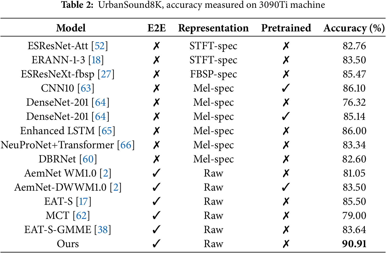
The UrbanSound8K dataset covers a wide range of audio categories, encompassing the richness of sound in urban environments. It is important to consider that in urban environments, sound characteristics are affected by factors such as background noise, environmental changes, and reverberation, resulting in more significant domain differences. The model should have a high generalization ability to adapt to diverse sound environments.

The experimental results, shown in Table 2, indicate that although [2] used an end-to-end model and combined it with a pre-trained model, the accuracy did not exceed that of a model based on Mel-spec (Mel spectrogram) as input [63]. Overall, the accuracy of the models based on raw audio as input [2,17] is still not as good as the models using Mel-spec as input [18,27,63], but it is slightly better compared to STFT-spec (Short Time Fourier Transform Spectrum) and FBSP-spec (Frequency Bandsplit Excitation Features). This is because Mel-spec transforms audio signals into frequency and time representations, which is closer to the way the human ear perceives audio. Our approach overcomes the problems of Mel-spec in terms of partial information loss during the conversion process and degradation of classification performance in human-computer interaction and noisy environments, and achieves significant performance improvement. Relative to the end-to-end model [17], our method achieves an even greater performance improvement of 5.28%. These results fully demonstrate the effectiveness of our method.

4.2.3 Comparison with Other Algorithms on the RAVDESS

Considering the need for human-computer interaction for human emotion recognition scenarios, we chose the RAVDESS dataset for our study. In this experiment, we compared the performance of the end-to-end model and the model using raw data as input. The experimental results shown in Table 3.

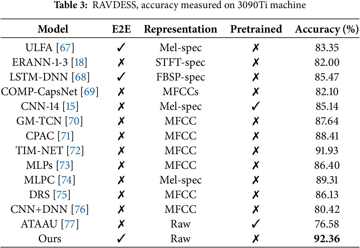
As we can seend in Table 3, the results indicate that the end-to-end model [67,68], and the model with raw data [77] as input are overall worse, which may be due to the difficulty of the RAVDESS dataset. This dataset contains rich expressions of human emotions, and emotion recognition itself is a complex task involving multiple aspects of speech such as tone, pitch, speech rate, and rhythm.

To address this situation, we compared the effectiveness of models using different vocal features as inputs and found that MFCC (Mel-Frequency Cepstral Coefficients) based models [70–72] generally outperformed other types of [18,67,68] inputs in terms of performance. This can be attributed to the properties of the MFCC, which utilizes the DCT (Discrete Cosine Transform) to compress the energy distribution of the Mel filter bank, thereby extracting key features and reducing the data dimensionality. In addition, by applying Mel filters in the frequency domain, MFCC is also able to reduce noise and redundant information, thus extracting more discriminative features. However, it should be noted that MFCC focuses only on frequency information, which may lose some time-domain features, as well as performs slightly less well when dealing with pitch variations.

To compensate for the shortcomings of MFCC, our model takes the above issues into account and improves the performance by 0.43% compared to previous studies [72]. Moreover, for the end-to-end model [68], we achieved a significant 6.89% improvement. All these results clearly demonstrate the effectiveness of our proposed approach.

4.2.4 Comparison with Other Algorithms on the CREMA-D

To further analyze the generalization capability of the proposed algorithm, we evaluated its performance on the more challenging multimodal emotion recognition dataset, CREMA-D. This experiment compared various model architectures and input data types, with the results presented in Table 4.

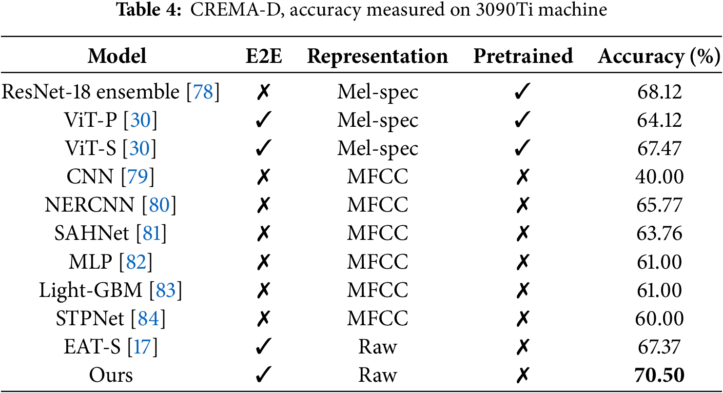
Models such as ResNet-18 ensemble [78] and ViT-P [30], which rely on Mel-spectrograms and pre-trained backbones, demonstrate limitations in leveraging audio information effectively, regardless of whether they use CNN or Transformer architectures. Similarly, MFCC-based models (e.g., NERCNN [80] and SAHNet [81]) show limited adaptability to diverse audio environments due to their restricted feature scope. It is noteworthy that MFCC primarily focuses on frequency information, which may result in the loss of some temporal features and suboptimal performance when handling pitch variations. Unlike traditional methods that depend on handcrafted features like MFCC or Mel-spectrograms, our model directly processes raw audio signals. The semantic branch and detail branch effectively handle complementary aspects of audio features, while the integration of the guided aggregation module ensures efficient fusion of multi-scale information from the two branches. Compared to previous studies, our model achieves a 2.38% improvement over ResNet-18 ensemble [78]. Additionally, it outperforms EAT-S [17], another end-to-end approach using raw audio, by 3.13%. These results clearly demonstrate the effectiveness of the proposed method and its robustness in tackling complex emotion recognition tasks.

4.2.5 Overall Performance and Discussion

To comprehensively evaluate the performance and stability of our model across different tasks, Table 5 presents the evaluation metrics for the four datasets. First, the model achieved its best performance on the ESC-50 dataset, with an Accuracy of 93.25% and an F1-Score of 93.02%. This demonstrates the model’s strong feature extraction capability and classification performance in environmental sound classification tasks. These results highlight the model’s ability to retain fine-grained information from raw audio and effectively leverage spatiotemporal features for precise classification. Similarly, the model also performed exceptionally well on the UrbanSound8K dataset, with all metrics exceeding 90%, including an F1-Score of 90.78%. This indicates the model’s robustness and generalization ability in urban noise scenarios, where it can adapt to complex background noise and diverse audio features.

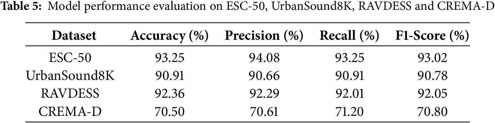
For speech emotion recognition, the model exhibited excellent performance on the multimodal RAVDESS dataset, achieving an Accuracy of 92.36% and an F1-Score of 92.05%. This demonstrates the model’s ability to effectively capture emotional features in speech. However, its performance on the more challenging CREMA-D dataset was relatively lower, with an Accuracy of 70.50%. The relatively lower performance on the CREMA-D dataset highlights the inherent challenges associated with emotion recognition tasks in this dataset. Compared to other datasets, CREMA-D features more complex emotion categories, diverse intensity levels of emotional expression, and significant variability among actors, which pose greater demands on the model’s generalization capabilities. Additionally, the short duration of audio clips in CREMA-D may lack sufficient contextual information, further complicating the modeling of temporal dependencies critical for accurate emotion recognition.

Further analysis reveals that the model demonstrates consistency in Precision, Recall, and F1-Score across all datasets, indicating high classification stability with no significant bias. This stability is particularly evident in environmental sound classification tasks (ESC-50 and UrbanSound8K), where the model’s robustness ensures reliable performance even in noisy environments. Moreover, the end-to-end dual-branch design allows the model to fully exploit the detailed information in raw audio signals, exhibiting strong generalization capabilities and adaptability across multiple tasks. To address the unique challenges posed by the CREMA-D dataset, future research can be directed toward the following aspects: First, the emotion feature extraction module can be optimized by incorporating dynamic modeling strategies to enhance the capture of complex temporal dependencies. Second, integrating visual modality information through multimodal fusion approaches could improve the understanding of emotional expressions by leveraging complementary cues from multiple sources. Finally, employing generative adversarial networks (GANs) to produce diverse training samples could help mitigate data imbalance issues and enhance the model’s robustness in handling the variability and complexity of the dataset.

The model’s computational efficiency was also evaluated. On a 3090Ti GPU, the memory usage for processing a single test sample was 2.3 GB, with an average inference time of 0.026 s. The low memory usage demonstrates the model’s efficiency in an end-to-end framework, making it well-suited for deployment on modern GPU hardware with sufficient memory capacity. Furthermore, the short inference time highlights the model’s potential applicability in real-time tasks. This efficiency can be attributed to the design of the Fast Downsampling Module (FDM) and the Multi-Scale Audio Context Embedding Module (MACEM), which effectively reduce computational complexity while maintaining classification performance. Additionally, the model eliminates the need for complex preprocessing steps, such as generating Mel-spectrograms or STFT-spectrograms, further reducing the computational overhead.

Although the proposed model demonstrates strong scalability and compatibility with various tasks, it has certain limitations that should be noted. First, the reliance on publicly available datasets such as ESC-50, UrbanSound8K, RAVDESS, and CREMA-D may not fully represent real-world scenarios, especially in terms of noise complexity and category diversity. Additionally, the model’s performance on tasks requiring highly detailed temporal context, such as speech generation or long-sequence modeling, may be limited by its architecture.

Furthermore, while the model is efficient on high-performance GPUs, its deployment on resource-constrained devices remains a challenge due to memory usage and inference speed. Although techniques such as quantization and pruning may address these issues, they were not explored in this study. Finally, the experiments primarily focus on controlled datasets, and the model’s generalization to real-world data or unseen audio domains has not been extensively verified.

4.3 Ablation Study on UrbanSound8K

To further investigate the effect of different sites on the classification results, we conducted an ablation study on the UrbanSound8K dataset. To demonstrate the effect of MACEM, and GARM, we conducted 10 experiments on it. First, we test the effect of not using any of the modules. Second, we test the effect of using only a single module separately. Again, we tested the effect of combining two and two, and finally, we tested the effect of using all three modules together. The results of the ablation study are shown in Table 6. We have the following observations.

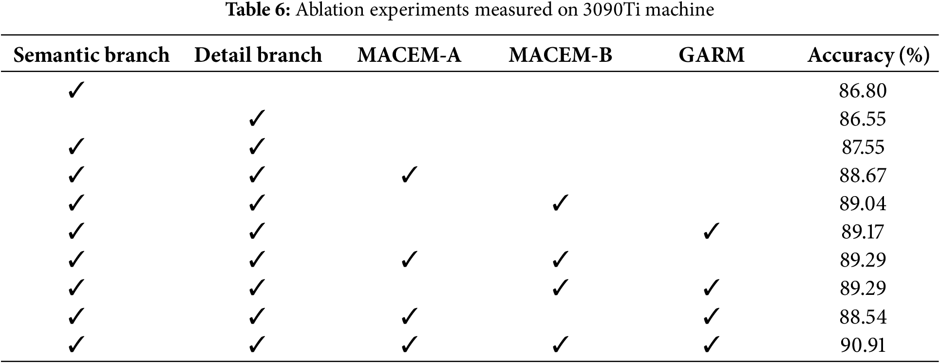
First, Table 6 shows that the three modules proposed in this paper have improved the model performance individually and in combination, achieving a +3.36% improvement when all modules are used.

The reason is that GARM not only focuses on the channel dimension but also on the time dimension, which can capture the internal and interconnection of different time scales and better aggregate the relationship between different time scales and internal contexts, compared with MACEM-A, which adopts the summation method for the captured multiscale temporal features. Compared to MACEM-A, which uses the summation of captured multiscale temporal features, the fusion of features by channel concat allows more helpful information, which is essential for network models with raw audio input. Both MACEM-A and MACEM-B alone have improved and proved that the multiscale feature extraction strategy is effective, and it needs to focus on the channel dimension after the fusion of multiscale features to extract the acquired rich in time and filter out a large amount of invalid information. At the same time, the residual structure is also effective in enhancing its robustness.

When combining two and two, MACEM-B and C combination works best at +1.74%, mainly because it extracts features containing rich detail information from the shallow and middle layers of the network containing rich information at multiple scales, thus allowing the network to obtain more information for classification later. Finally, using multiple scales to extract different temporal features can better solve the problem of the need for more connection between the contexts of long sequences of raw audio input.

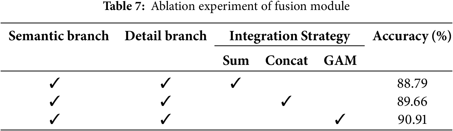
In the final stage of the double branching, we need to fuse the output features of these two paths, and considering the different levels of features, in terms of semantics and size, we propose the guided aggregation modulee(GAM) to fuse the features of these two paths effectively. First, we evaluate the effect of simple summing and concation of these features and our proposed feature fusion module, as shown in Table 7. The difference in comparative performance illustrates that the features of the two paths belong to different levels and the effectiveness of our designed fusion module.

4.4 Visualization

In the previous section, quantitative analysis demonstrated the performance of our model. In this section, we further qualitatively evaluate the model through visualization. Fig. 7 presents the two-dimensional distribution of features from the UrbanSound8K test set after dimensionality reduction using t-SNE.

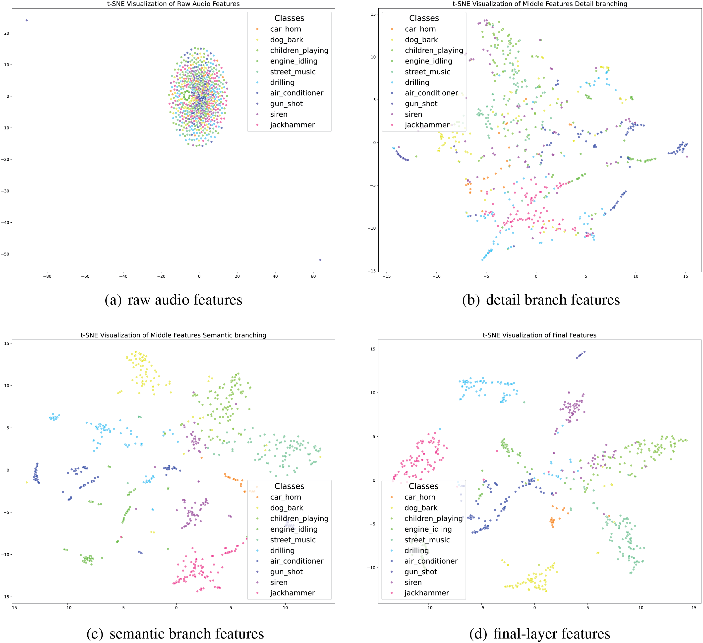
Figure 7: Different colors represent the 10 categories of sound samples in the dataset, namely air_conditioner, car_horn, children_playing, dog_bark, drilling, engine_idling, gun_shot, jackhammer, siren, street_music

Regarding inter-class separability, the distribution of raw audio features (Fig. 7a) shows significant overlap between classes, with many categories, such as car_horn and siren, exhibiting severe mixing. This is because raw audio contains substantial redundancy and noise, making it challenging for the model to distinguish between categories. In contrast, the features extracted by the detail branch (Fig. 7b) show noticeable improvement compared to Fig. 7a. Certain categories, such as engine_idling and jackhammer, begin to separate, though some overlap remains. This indicates that the detail branch effectively captures temporal details but has limited ability to model global semantic information. The features extracted by the semantic branch (Fig. 7c) exhibit better inter-class separation than those from the detail branch, with some categories, such as dog_bark and children_playing, forming relatively distinct clusters. This demonstrates that the semantic branch can model high-level semantic information effectively, albeit potentially at the cost of finer details. The final-layer features (Fig. 7d) combine the strengths of both branches, achieving the best inter-class separability. Most categories form compact clusters and are clearly separated in the two-dimensional space, with only minor overlaps in a few categories, such as street_music and siren. This highlights the effectiveness of the fusion strategy in significantly improving the overall feature extraction capability, addressing the limitations of single-branch approaches.

After analyzing inter-class separability, we further examine the model’s performance in terms of intra-class compactness. The intra-class distribution of raw audio features (Fig. 7a) is sparse, with significant distances between data points, indicating that the model struggles to capture common characteristics among samples of the same class. The intermediate features extracted by the two branches (Fig. 7b and c) show improvement, with Fig. 7b demonstrating modest intra-class compactness, though not as strong as Fig. 7c. The semantic branch is more effective in compressing the distribution of samples within the same class. The final-layer features (Fig. 7d) achieve the best intra-class compactness, with samples from the same class forming high-density clusters in the two-dimensional space. This demonstrates that the fusion strategy not only enhances inter-class separability but also significantly improves intra-class consistency.

Through the comparative analysis of the four t-SNE visualizations, we observe that raw audio features (Fig. 7a) contain substantial redundancy and make class distinction difficult. The detail branch (Fig. 7b) focuses on capturing temporal details, enabling initial separation of some categories. The semantic branch (Fig. 7c) emphasizes semantic information, significantly improving inter-class separation. Finally, the dual-branch fusion strategy successfully combines the strengths of both branches in the final-layer features (Fig. 7d), achieving optimal inter-class separability and intra-class compactness.

The t-SNE visualizations intuitively demonstrate the classification performance of our model on the UrbanSound8K dataset. Overall, the model achieves excellent clustering and separation for most categories, indicating that the feature extraction module effectively captures inter-class differences. However, for overlapping categories, such as street_music and **siren**, future research could explore more advanced feature extraction techniques, such as multimodal feature fusion or contextual information modeling, to further improve classification performance.

5  Conclusion

This study proposes a novel end-to-end audio classification framework, which demonstrates outstanding performance on raw audio signals. Specifically, the Multi-Scale Audio Context Embedding Module aggregates temporal and spatial information across multiple scales, significantly enhancing the model’s adaptability to diverse audio signals. The Global Audio Refinement Module further improves global modeling capabilities by effectively integrating multi-scale channel and temporal information. Finally, the Guided Aggregation Module efficiently fuses complementary information from the semantic and detail branches. Experimental results show that our method outperforms state-of-the-art approaches on the ESC-50, UrbanSound8K, RAVDESS, and CREMA-D datasets. Furthermore, visualization analysis of the results reveals that the model excels in capturing intra-class compactness and inter-class separability, providing additional validation for its effectiveness.

Nevertheless, the model leaves room for improvement in handling emotion recognition tasks, particularly when dealing with complex emotional categories or integrating multimodal data. Future research will focus on optimizing the emotion feature extraction module and exploring joint modeling of multimodal information. Additionally, leveraging model lightweighting techniques such as quantization, pruning, or knowledge distillation could further enhance the framework’s applicability on resource-constrained devices.

Acknowledgement: This work was supported by the National Natural Science Foundation of China, the Hebei Natural Science Foundation, and the Provincial Key Laboratory Performance Subsidy Project.

Funding Statement: This work was supported by the National Natural Science Foundation of China (62106214), the Hebei Natural Science Foundation (D2024203008), and the Provincial Key Laboratory Performance Subsidy Project (22567612H).

Author Contributions: The authors confirm contribution to the paper as follows: study conception and design: Zijain Sun, Haoran Liu; data collection: Haibin Li; analysis and interpretation of results: Wenming Zhang; draft manuscript preparation: Yaqian Li. All authors reviewed the results and approved the final version of the manuscript.

Availability of Data and Materials: All data sets mentioned in Section 4 are publicly available, assuring replicability and availability for future research. These datasets are linked below: https://github.com/karolpiczak/ESC-50 (accessed on 17 February 2025); https://urbansounddataset.weebly.com/ (accessed on 17 February 2025); https://zenodo.org/record/1188976?continueFlag=b7c22bb40d2598cd01a707dc56266437 (accessed on 17 February 2025).

Ethics Approval: Not applicable.

Conflicts of Interest: The authors declare no conflicts of interest to report regarding the present study.

References

1. Chen K, Du X, Zhu B, Ma Z, Berg-Kirkpatrick T, Dubnov S. HTS-AT: a hierarchical token-semantic audio transformer for sound classification and detection. In: ICASSP 2022—2022 IEEE International Conference on Acoustics, Speech and Signal Processing (ICASSP); 2022 May 23–27; Singapore: IEEE; 2022. p. 646–50. doi:10.1109/ICASSP43922.2022.9746312. [Google Scholar] [CrossRef]

2. Lopez-Meyer P, del Hoyo Ontiveros JA, Lu H, Stemmer G. Efficient end-to-end audio embeddings generation for audio classification on target applications. In: ICASSP 2021—2021 IEEE International Conference on Acoustics, Speech and Signal Processing (ICASSP); 2021 Jun 6–11; Toronto, ON, Canada: IEEE; 2021. p. 601–5. doi:10.1109/icassp39728.2021.9414229. [Google Scholar] [CrossRef]

3. Abdoli S, Cardinal P, Lameiras Koerich A. End-to-end environmental sound classification using a 1D convolutional neural network. Expert Syst Appl. 2019;136(1):252–63. doi:10.1016/j.eswa.2019.06.040. [Google Scholar] [CrossRef]

4. Tho Nguyen TN, Jones DL, Watcharasupat KN, Phan H, Gan WS. SALSA-lite: a fast and effective feature for polyphonic sound event localization and detection with microphone arrays. In: ICASSP 2022—2022 IEEE International Conference on Acoustics, Speech and Signal Processing (ICASSP); 2022 May 23–27; Singapore: IEEE; 2022. p. 716–20. doi:10.1109/ICASSP43922.2022.9746132. [Google Scholar] [CrossRef]

5. Yang D, Wang H, Zou Y, Ye Z, Wang W. A mutual learning framework for few-shot sound event detection. In: ICASSP 2022–2022 IEEE International Conference on Acoustics, Speech and Signal Processing (ICASSP); 2022 May 23–27; Singapore: IEEE; 2022. p. 811–5. doi:10.1109/ICASSP43922.2022.9746042. [Google Scholar] [CrossRef]

6. Tian J, She Y. A visual-audio-based emotion recognition system integrating dimensional analysis. IEEE Trans Comput Soc Syst. 2023;10(6):3273–82. doi:10.1109/TCSS.2022.3200060. [Google Scholar] [CrossRef]

7. Aggarwal A, Srivastava A, Agarwal A, Chahal N, Singh D, Ali Alnuaim A, et al. Two-way feature extraction for speech emotion recognition using deep learning. Sensors. 2022;22(6):2378. doi:10.3390/s22062378. [Google Scholar] [PubMed] [CrossRef]

8. İnik Ö. CNN hyper-parameter optimization for environmental sound classification. Appl Acoust. 2023;202:109168. doi:10.1016/j.apacoust.2022.109168. [Google Scholar] [CrossRef]

9. Tang Q, Xu L, Zheng B, He C. Transound: hyper-head attention transformer for birds sound recognition. Ecol Inform. 2023;75(1):102001. doi:10.1016/j.ecoinf.2023.102001. [Google Scholar] [CrossRef]

10. Aghajani K. Audio-visual emotion recognition based on a deep convolutional neural network. J AI Data Mining. 2022;10(4):529–37. doi:10.22044/jadm.2022.11809.2331. [Google Scholar] [CrossRef]

11. Ali Alnuaim A, Zakariah M, Alhadlaq A, Shashidhar C, Atef Hatamleh W, Tarazi H, et al. Human-computer interaction with detection of speaker emotions using convolution neural networks. Comput Intell Neurosci. 2022;2022:7463091. doi:10.1155/2022/7463091. [Google Scholar] [PubMed] [CrossRef]

12. Alnuaim AA, Zakariah M, Shukla PK, Alhadlaq A, Hatamleh WA, Tarazi H, et al. Human-computer interaction for recognizing speech emotions using multilayer perceptron classifier. J Healthc Eng. 2022;2022:6005446. doi:10.1155/2022/6005446. [Google Scholar] [PubMed] [CrossRef]

13. Wöllmer M, Metallinou A, Eyben F, Schuller B, Narayanan S. Context-sensitive multimodal emotion recognition from speech and facial expression using bidirectional LSTM modeling. In: Interspeech 2010; 2010 Sep 26–30; Makuhari, Japan: ISCA; 2010. p. 2362–5. doi:10.21437/Interspeech.2010. [Google Scholar] [CrossRef]

14. Mukhamediya A, Fazli S, Zollanvari A. On the effect of log-mel spectrogram parameter tuning for deep learning-based speech emotion recognition. IEEE Access. 2023;11:61950–7. doi:10.1109/ACCESS.2023.3287093. [Google Scholar] [CrossRef]

15. Luna-Jiménez C, Griol D, Callejas Z, Kleinlein R, Montero JM, Fernández-Martínez F. Multimodal emotion recognition on ravdess dataset using transfer learning. Sensors. 2021;21(22):7665. doi:10.3390/s21227665. [Google Scholar] [PubMed] [CrossRef]

16. Davis S, Mermelstein P. Comparison of parametric representations for monosyllabic word recognition in continuously spoken sentences. IEEE Trans Acoust Speech Signal Process. 1980;28(4):357–66. doi:10.1109/tassp.1980.1163420. [Google Scholar] [CrossRef]

17. Gazneli A, Zimerman G, Ridnik T, Sharir G, Noy A. End-to-end audio strikes back: boosting augmentations towards an efficient audio classification network. arXiv:2204.11479. 2020. [Google Scholar]

18. Verbitskiy S, Berikov V, Vyshegorodtsev V. ERANNs: efficient residual audio neural networks for audio pattern recognition. Pattern Recognit Lett. 2022;161(5):38–44. doi:10.1016/j.patrec.2022.07.012. [Google Scholar] [CrossRef]

19. Li J, Dai W, Metze F, Qu S, Das S. A comparison of deep learning methods for environmental sound detection. In: 2017 IEEE International Conference on Acoustics, Speech and Signal Processing (ICASSP); 2017 Mar 5–9; New Orleans, LA, USA: IEEE; 2017. p. 126–30. doi:10.1109/ICASSP.2017.7952131. [Google Scholar] [CrossRef]

20. Chen Y, Zhu Y, Yan Z, Ren Z, Huang Y, Shen J, et al. Effective audio classification network based on paired inverse pyramid structure and dense MLP Block. In: International Conference on Intelligent Computing; 2023 Aug 10–13; Singapore; 2023. p. 70–84. [Google Scholar]

21. Zouhir Y, Ouni K. Feature extraction method for improving speech recognition in noisy environments. J Comput Sci. 2016;12(2):56–61. doi:10.3844/jcssp.2016.56.61. [Google Scholar] [CrossRef]

22. Valero X, Alias F. Gammatone cepstral coefficients: biologically inspired features for non-speech audio classification. IEEE Trans Multimedia. 2012;14(6):1684–9. doi:10.1109/tmm.2012.2199972. [Google Scholar] [CrossRef]

23. Zhou X, Garcia-Romero D, Duraiswami R, Espy-Wilson C, Shamma S. Linear versus mel frequency cepstral coefficients for speaker recognition. In: 2011 IEEE Workshop on Automatic Speech Recognition & Understanding; 2011 Dec 11–15; Waikoloa, HI, USA: IEEE; 2011. p. 559–64. doi:10.1109/ASRU.2011.6163888. [Google Scholar] [CrossRef]

24. Kumar C, ur Rehman F, Kumar S, Mehmood A, Shabir G. Analysis of MFCC and BFCC in a speaker identification system. In: International Conference on Computing, Mathematics and Engineering Technologies (iCoMET); 2018 Mar 3–4; Sukkur, Pakistan: IEEE; 2018. p. 1–5. doi:10.1109/ICOMET.2018.8346330. [Google Scholar] [CrossRef]

25. Mushtaq Z, Su S-F, Tran Q-V. Spectral images based environmental sound classification using CNN with meaningful data augmentation. Appl Acoust. 2021 Jan;172(2):107581. doi:10.1016/j.apacoust.2020.107581. [Google Scholar] [CrossRef]

26. Qin W, Yin B. Environmental sound classification algorithm based on adaptive data padding. In: 2022 International Seminar on Computer Science and Engineering Technology (SCSET); 2022 Jan 8–9; Indianapolis, IN, USA: IEEE; 2022. p. 84–8. doi:10.1109/SCSET55041.2022.00028. [Google Scholar] [CrossRef]

27. Guzhov A, Raue F, Hees J, Dengel A. ESResNe(X)t-fbsp: learning robust time-frequency transformation of audio. In: 2021 International Joint Conference on Neural Networks (IJCNN); 2021 Jul 18–22; Shenzhen, China: IEEE; 2021. p. 1–8. doi:10.1109/IJCNN52387.2021.9533654. [Google Scholar] [CrossRef]

28. Zhang H, Huang H, Zhao P, Zhu X, Yu Z. CENN: capsule-enhanced neural network with innovative metrics for robust speech emotion recognition. Knowl Based Syst. 2024;304:112499. doi:10.1016/j.knosys.2024.112499. [Google Scholar] [CrossRef]

29. Tokozume Y, Harada T. Learning environmental sounds with end-to-end convolutional neural network. In: 2017 IEEE International Conference on Acoustics, Speech and Signal Processing (ICASSP); 2017 Mar 5–7; New Orleans, LA, USA: IEEE; 2017. p. 2721–5. [Google Scholar]

30. Gong Y, Chung Y-A, Glass J. AST: audio spectrogram transformer. In: Interspeech 2021, 22nd Annual Conference of the International Speech Communication Association; 2021; Brno, Czechia. p. 571–5. [Google Scholar]

31. Chen J, Ma X, Li S, Ma S, Zhang Z, Ma X. A hybrid parallel computing architecture based on CNN and transformer for music genre classification. Electronics. 2024;13(16):3313. doi:10.3390/electronics13163313. [Google Scholar] [CrossRef]

32. Li Q, Hu B. Joint time and frequency transformer for chinese opera classification. In: Proceedings of the Interspeech; 2023. p. 3919–23. doi:10.21437/interspeech.2023-1582. [Google Scholar] [CrossRef]

33. Tang R, Qi M, Wang N. Music style classification by jointly using CNN and Transformer. In: Proceedings of the 2024 16th International Conference on Machine Learning and Computing; 2024; Shenzhen, China: ACM; 2024. p. 707–12. doi:10.1145/3651671.3651696. [Google Scholar] [CrossRef]

34. Mangalmurti S, Saxena O, Singh T. Speech emotion recognition using CNN-TRANSFORMER architecture. In: 2024 IEEE International Conference on Interdisciplinary Approaches in Technology and Management for Social Innovation (IATMSI); 2024 Mar 14–16; Gwalior, India: IEEE; 2024. p. 1–6. doi:10.1109/IATMSI60426.2024.10503276. [Google Scholar] [CrossRef]

35. Tellai M, Gao L, Mao Q. An efficient speech emotion recognition based on a dual-stream CNN-transformer fusion network. Int J Speech Technol. 2023;26(2):541–57. doi:10.1007/s10772-023-10035-y. [Google Scholar] [CrossRef]

36. Zhang S, Gao Y, Cai J, Yang H, Zhao Q, Pan F. A novel bird sound recognition method based on multifeature fusion and a transformer encoder. Sensors. 2023;23(19):8099. doi:10.3390/s23198099. [Google Scholar] [PubMed] [CrossRef]

37. Peng Z, Lu Y, Pan S, Liu Y. Efficient speech emotion recognition using multi-scale cnn and attention. In: ICASSP 2021—2021 IEEE International Conference on Acoustics, Speech and Signal Processing (ICASSP); 2021 Jun 6–11; Toronto, ON, Canada: IEEE; 2021. p. 3020–4. doi:10.1109/icassp39728.2021.9414286. [Google Scholar] [CrossRef]

38. He B, Zhang S, Wang X, Qiu Z, Takeuchi D, Niizumi D, et al. Light gated multi mini-patch extractor for audio classification. In: 2024 IEEE International Conference on Acoustics, Speech, and Signal Processing Workshops (ICASSPW); 2024 Apr 14–19; Seoul, Republic of Korea: IEEE; 2024. p. 765–9. doi:10.1109/ICASSPW62465.2024.10626081. [Google Scholar] [CrossRef]

39. Ioffe S, Szegedy C. Batch normalization: accelerating deep network training by reducing internal covariate shift. Vol. 37. In: 32nd International Conference on Machine Learning; 2015 Jul 6–11; Lille, France: ACM; 2015. p. 448–56. doi:10.5555/3045118.3045167. [Google Scholar] [CrossRef]

40. Maas AL, Hannun AY, Ng AY. Rectifier nonlinearities improve neural network acoustic models. In: Proceedings of the 30th International Conference on Machine Learning; 2013 Jun 16–21; Atlanta, GA, USA; 2013. [Google Scholar]

41. Hochreiter S, Schmidhuber J. Long short-term memory. Neural Comput. 1997;9(8):1735–80. doi:10.1162/neco.1997.9.8.1735. [Google Scholar] [PubMed] [CrossRef]

42. Vaswani A, Shazeer N, Parmar N, Uszkoreit J, Jones L, Gomez AN, et al. Attention is all you need. In: Advances in Neural Information Processing Systems; 2017 Dec 4–9; Long Beach, CA, USA; 2017. [Google Scholar]

43. Piczak KJ. ESC: dataset for environmental sound classification. In: Proceedings of the 23rd ACM/IEEE International Conference; 2015 Oct 26–30; Brisbane, Australia: ACM; 2015. p. 1015–8. doi:10.1145/2733373.2806390. [Google Scholar] [CrossRef]

44. Salamon J, Jacoby C, Bello JP. A dataset and taxonomy for urban sound research. In: Proceedings of the 22nd ACM International Conference on Multimedia; 2014 Nov 3–7; Orlando, FL, USA: ACM; 2014. p. 1041–4. doi:10.1145/2647868.2655045. [Google Scholar] [CrossRef]

45. Livingstone SR, Russo FA. The ryerson audio-visual database of emotional speech and song (RAVDESSa dynamic, multimodal set of facial and vocal expressions in North American English. PLoS One. 2018;13(5):e0196391. doi:10.1371/journal.pone.0196391. [Google Scholar] [PubMed] [CrossRef]

46. Cao H, Cooper DG, Keutmann MK, Gur RC, Nenkova A, Verma R. CREMA-D: crowd-sourced emotional multimodal actors dataset. IEEE Trans Affect Comput. 2014;5(4):377–90. doi:10.1109/taffc.2014.2336244. [Google Scholar] [PubMed] [CrossRef]

47. Loshchilov I, Hutter F. Decoupled weight decay regularization. arXiv:1711.05101. 2017. [Google Scholar]

48. Smith LN. A disciplined approach to neural network hyper-parameters: part 1—learning rate, batch size, momentum, and weight decay. arXiv:1803.09820. 2018. [Google Scholar]

49. Tarvainen A, Valpola H. Mean teachers are better role models: weight-averaged consistency targets improve semi-supervised deep learning results. Adv Neural Inform Process Syst. 2017;30:1195–204. [Google Scholar]

50. Izmailov P, Podoprikhin D, Garipov T, Vetrov D, Wilson AG. Averaging weights leads to wider optima and better generalization. In: Conference on Uncertainty in Artificial Intelligence (UAI); 2018 Aug 6–10; Monterey, CA, USA; 2018. p. 876–85. [Google Scholar]

51. Zhang L, Song J, Gao A, Chen J, Bao C, Ma K. Be Your Own Teacher: improve the performance of convolutional neural networks via self distillation. In: 2019 IEEE/CVF International Conference on Computer Vision (ICCV); 2019 Oct 27–Nov 2; Seoul, Republic of Korea: IEEE; 2019. p. 3712–21. doi:10.1109/ICCV.2019.00381. [Google Scholar] [CrossRef]

52. Guzhov A, Raue F, Hees J, Dengel A. ESResNet: environmental sound classification based on visual domain models. In: 2020 25th International Conference on Pattern Recognition (ICPR); 2021; Milan, Italy: IEEE. p. 4933–40. doi:10.1109/ICPR48806.2021.9413035. [Google Scholar] [CrossRef]

53. Zhu B, Xu K, Wang D, Zhang L, Li B, Peng Y. Environmental sound classification based on multi-temporal resolution convolutional neural network combining with multi-level features. In: Advances in Multimedia Information Processing—PCM 2018: 19th Pacific-Rim Conference on Multimedia; 2018 Sep 21–22; Hangzhou, China; 2018. p. 528–37. [Google Scholar]

54. Tokozume Y, Ushiku Y, Harada T. Learning from between-class examples for deep sound recognition. In: International Conference on Learning Representations (ICLR); 2018; Vancouver, BC, Canada. p. 1–13. [Google Scholar]

55. Liu X, Liu H, Kong Q, Mei X, Plumbley MD, Wang W. Simple pooling front-ends for efficient audio classification. In: ICASSP 2023—2023 IEEE International Conference on Acoustics, Speech and Signal Processing (ICASSP); 2023 Jun 4–10; Rhodes Island, Greece: IEEE; 2023. p. 1–5. doi:10.1109/ICASSP49357.2023.10096211. [Google Scholar] [CrossRef]

56. Yu Z, Wang S, Chen L, Cheng Z. Halluaudio: hallucinate frequency as concepts for few-shot audio classification. In: ICASSP 2023—2023 IEEE International Conference on Acoustics, Speech and Signal Processing (ICASSPRhodes Island; 2023 Jun 4–10; Rhodes Island, Greece: IEEE; 2023. p. 1–5. doi:10.1109/ICASSP49357.2023.10095663. [Google Scholar] [CrossRef]

57. Wang C, Ito A, Nose T, Chen C-P. Evaluation of environmental sound classification using vision transformer. In: Proceedings of the 2024 16th International Conference on Machine Learning and Computing; 2024; New York, NY, USA: ACM; 2024. p. 665–9. doi:10.1145/3651671.3651733. [Google Scholar] [CrossRef]

58. Gouläo M, Bandeira L, Martins B, Oliveira AL. Training environmental sound classification models for real-world deployment in edge devices. Discov Appl Sci. 2024;6(4):166. doi:10.1007/s42452-024-05803-7. [Google Scholar] [CrossRef]

59. Pasha SMM, Sohag SR, Ali MM. Enhancing audio classification with a CNN-attention model: robust performance and resilience against backdoor attacks. Int J Comput Appl. 2024;186(49):975. doi:10.5120/ijca2024924154. [Google Scholar] [CrossRef]

60. Zhang D, Zhong Z, Xia Y, Wang Z, Xiong W. An automatic classification system for environmental sound in smart cities. Sensors. 2023;23(15):6823. doi:10.3390/s23156823. [Google Scholar] [PubMed] [CrossRef]

61. Mohaimenuzzaman M, Bergmeir C, West I, Meyer B. Environmental sound classification on the edge: a pipeline for deep acoustic networks on extremely resource-constrained devices. Pattern Recognit. 2023 Jan;133(2):109025. doi:10.1016/j.patcog.2022.109025. [Google Scholar] [CrossRef]

62. Mou A, Milanova M. Performance analysis of deep learning model-compression techniques for audio classification on edge devices. Sci. 2024;6(2):21. doi:10.3390/sci6020021. [Google Scholar] [CrossRef]

63. Arnault A, Hanssens B, Riche N. Urban sound classification: striving towards a fair comparison. arXiv:2010.11805. 2020. [Google Scholar]

64. Palanisamy K, Singhania D, Yao A. Rethinking CNN models for audio classification. arXiv:2007.11154. 2020. [Google Scholar]

65. Tyagi S, Aggarwal K, Kumar D, Garg S. Urban sound classification for audio analysis using long short term memory. NEU J Artif Intell Internet Things. 2023;1(2):1–11. [Google Scholar]

66. Tran K-T, Vu X-S, Nguyen K, Nguyen HD. NeuProNet: neural profiling networks for sound classification. Neural Comput Appl. 2024;36(11):5873–87. doi:10.1007/s00521-023-09361-8. [Google Scholar] [CrossRef]

67. Mocanu B, Tapu R, Zaharia T. Utterance level feature aggregation with deep metric learning for speech emotion recognition. Sensors. 2021;21(12):4233. doi:10.3390/s21124233. [Google Scholar] [PubMed] [CrossRef]

68. Senthilkumar N, Karpakam S, Devi MG, Balakumaresan R, Dhilipkumar P. Speech emotion recognition based on Bi-directional LSTM architecture and deep belief networks. Mater Today: Proc. 2022;57(5):2180–4. doi:10.1016/j.matpr.2021.12.246. [Google Scholar] [CrossRef]

69. Shahin I, Hindawi N, Nassif AB, Alhudhaif A, Polat K. Novel dual-channel long short-term memory compressed capsule networks for emotion recognition. Expert Syst Appl. 2022;188(4):116080. doi:10.1016/j.eswa.2021.116080. [Google Scholar] [CrossRef]

70. Ye JX, Wen XC, Wang XZ, Xu Y, Luo Y, Wu CL, et al. GM-TCNet: gated multi-scale temporal convolutional network using emotion causality for speech emotion recognition. Speech Commun. 2022 Nov;145(2):21–35. doi:10.1016/j.specom.2022.07.005. [Google Scholar] [CrossRef]

71. Wen XC, Ye JX, Luo Y, Xu Y, Wang XZ, Wu CL, et al. CTL-MTNet: a novel CapsNet and transfer learning-based mixed task net for single-corpus and cross-corpus speech emotion recognition. In: Proceedings of the Thirty-First International Joint Conference on Artificial Intelligence; 2022 Jul 23–29; Vienna, Austria: International Joint Conferences on Artificial Intelligence Organization; 2022. p. 2305–11. doi:10.24963/ijcai.2022/320. [Google Scholar] [CrossRef]

72. Ye J, Wen XC, Wei Y, Xu Y, Liu K, Shan H. Temporal modeling matters: a novel temporal emotional modeling approach for speech emotion recognition. In: ICASSP 2023—2023 IEEE International Conference on Acoustics, Speech and Signal Processing (ICASSP); 2023 Jun 4–10; Rhodes Island, Greece: IEEE; 2023. p. 1–5. doi:10.1109/ICASSP49357.2023.10096370. [Google Scholar] [CrossRef]

73. Ammanavar Y, Patil S, Bidargaddi AP, Deshanur P, Rathod R, Meena SM. Speech emotion recognition on RAVDESS dataset using deep learning. In: 2024 5th International Conference for Emerging Technology (INCET); 2024 May 24–26; Belgaum, India: IEEE; 2024. p. 1–6. doi:10.1109/INCET61516.2024.10593471. [Google Scholar] [CrossRef]

74. Advaith KS. Enhancing speech audio emotion recognition for diverse feature analysis through MLP classifier. In: 2024 International Conference on Cognitive Robotics and Intelligent Systems (ICC-ROBINS); 2024 Apr 17–19; Coimbatore, India: IEEE; 2024. p. 656–62. doi:10.1109/ICC-ROBINS60238.2024.10533912. [Google Scholar] [CrossRef]

75. Das AK, Naskar R. A deep learning model for depression detection based on MFCC and CNN generated spectrogram features. Biomed Signal Process Control. 2024;90:105898. [Google Scholar]

76. Mishra SP, Warule P, Deb S. Speech emotion classification using feature-level and classifier-level fusion. Evol Syst. 2024;15(2):541–54. doi:10.1007/s12530-023-09550-9. [Google Scholar] [CrossRef]

77. Luna-Jiménez C, Kleinlein R, Griol D, Callejas Z, Montero JM, Fernández-Martínez F. A proposal for multimodal emotion recognition using aural transformers and action units on RAVDESS dataset. Appl Sci. 2022;12(1):327. doi:10.3390/app12010327. [Google Scholar] [CrossRef]

78. Ristea NC, Ionescu RT. Self-paced ensemble learning for speech and audio classification. arXiv:2103.11988. 2021. [Google Scholar]

79. Marcos L, Mai KV, Abhari A. Emotion classification through speech data analysis. In: 2023 Winter Simulation Conference (WSC); 2023 Dec 10–13; San Antonio, TX, USA: IEEE; 2023. p. 2908–19. doi:10.1109/WSC60868.2023.10408424. [Google Scholar] [CrossRef]

80. Mekruksavanich S, Jitpattanakul A, Hnoohom N. Negative emotion recognition using deep learning for thai language. In: 2020 Joint International Conference on Digital Arts, Media and Technology with ECTI Northern Section Conference on Electrical, Electronics, Computer and Telecommunications Engineering (ECTI DAMT & NCON); 2020 Mar 11–14; Pattaya, Thailand: IEEE; 2020. p. 71–4. doi:10.1109/ectidamtncon48261.2020.9090768. [Google Scholar] [CrossRef]

81. Savla M, Gopani D, Ghuge M, Chaudhari S, Raundale P. Sentiment analysis of human speech using deep learning. In: 2023 3rd International Conference on Intelligent Technologies (CONIT); 2023 Jun 23–25; Hubli, India: IEEE; 2023. p. 1–6. doi:10.1109/CONIT59222.2023.10205915. [Google Scholar] [CrossRef]

82. Kumar P, Khera R, Grover A, Sharma K. Exploring speech emotion recognition with MLP classifier: a comprehensive study on the CREMA-D dataset. In: 2024 IEEE 4th International Conference on Smart Information Systems and Technologies (SIST); 2024 May 15–17; Astana, Kazakhstan: IEEE; 2023. p. 542–7. doi:10.1109/SIST61555.2024.10629409. [Google Scholar] [CrossRef]

83. Duong BV, Ha CN, Nguyen TT, Nguyen P, Do TH. An empirical experiment on feature extractions based for speech emotion recognition. In: Asian Conference on Intelligent Information and Database Systems; 2022 Nov 28–30; Cham: Springer Nature Switzerland; 2022. p. 180–91. [Google Scholar]

84. Hidayati SC, Adidarma AS, Sungkono KR. Exploring the impact of spatio-temporal patterns in audio spectrograms on emotion recognition. In: 2023 International Conference on Advanced Mechatronics, Intelligent Manufacture and Industrial Automation (ICAMIMIA); 2023 Nov 14–15; Surabaya, Indonesia: IEEE; 2023. p. 200–5. doi:10.1109/ICAMIMIA60881.2023.10427930. [Google Scholar] [CrossRef]