Ensemble of Deep Learning with Crested Porcupine Optimizer Based Autism Spectrum Disorder Detection Using Facial Images

1  Introduction

Autism spectrum disorders (ASD) denote a set of intricate neuro-developmental brain diseases like Asperger’s disorders, autism, and childhood disintegrative syndromes that, as the phrase “spectrum” involves, possess a great variety of symptoms and severity levels [1]. This disease is now incorporated in the International Statistical Diseases Classification and Relevant Health Difficulties under Behavioral and Mental Disorders, as part of Pervasive Developmental Conditions. The primary signs of ASD frequently seem to be in the 1st stage of life and can contain low levels of eye contact, a lack of response to calling their name, and unimportance to caretakers [2]. Very few children seem to grow normally in the 1st year and later indicate symptoms of autism between 18–24 months age groups, containing narrow and repetitive behaviour patterns, limited range of activities and interests, and insufficiency in verbal communication [3]. Such conditions also have an impact on how a person notices and mingles with other people, Children can unintentionally exhibit aggression or introversion throughout the first five years of life as they navigate challenges in communication and social interaction. However, ASD examines childhood and extends its focus into adolescence and adulthood [4].

Artificial intelligence (AI) has identified decision-making speed and it decreases the time needed to establish a diagnosis compared with classic diagnosis methods for detecting autism in the primary phase of life [5]. The transformation in diagnosing autism is physical, and it depends on psychologically noticing the child’s behaviour for a long time [6]. Occasionally these challenges take a maximum of two sessions. To diagnose autism, technology development has allowed the growth of diagnostic and screening mechanisms. The development of AI has headed to its better usage in the domain of medical and health care, and investigators are very busy with emerging techniques to detect ASD and identify autism at a very young age with diverse techniques namely eye contact, brain (magnetic resonance imaging) MRI, electroencephalogram (EEG) signals, and eye tracking. Some investigators have applied facial features to identify autism [7]. This study introduces an Ensemble of deep learning models based on the autism spectrum disorder detection in facial images (EDLM-ASDDFI) model. In the EDLM-ASDDFI method, the primary level of data pre-processing is involved in Gabor filtering (GF). Besides, the EDLM-ASDDFI technique applies the MobileNetV2 model to learn complex features from the pre-processed data. For the ASD detection process, the EDLM-ASDDFI method uses ensemble techniques for the classification procedure that encompasses the hyperparameter selection of the three DL models, which can be implemented by the design of the crested porcupine optimizer (CPO) technique. An extensive experiment was conducted to emphasize the improved ASD detection performance of the EDLM-ASDDFI method.

Alhakbani [8] introduced an automated engagement detection method using facial emotional recognition, especially in identifying the engagement of autistic children. The method used a transfer learning (TL) method at the dataset levels, using the datasets of facial images from typically developing (TD) children with ASD and children. The identification tasks are executed using CNN techniques. Thanarajan et al. [9] aim to enhance the efficacy of deep learning (DL) hybrid methods, like vision transformer (ViT) integrated with support vector machine (SVM) and principal component analysis (PCA), VGG16 with Extreme Gradient Boosting (XGBoost), ViT with CatBoost, and ViT with XGBoost. These changes are particularly designed for image identification tasks, like identifying ASD in toddlers’ facial images. In [10], an ASD recognition hybrid method is proposed that is based on 2 different datasets. At first, behaviour datasets worked on the logistic regression (LR) method, and in addition, facial datasets worked on convolutional neural network (CNN) classification to forecast whether an individual has suffered from autism or not. Khan et al. [11] examined this to help both psychiatrists and families in analyzing autism by a simple method. In particular, the research uses a DL technique, which uses empirically verified facial features. The method contains a CNN with TL for autism detections. DenseNet-121, VGG16, ResNet-50, Xception, and MobileNetV2 are the pre-trained methods employed for autism detection. Vidyadhari et al. [12] focus on ASD detection by Deep Quantum Neural Networks (DQNNs), where these networks are trained by a presented fractional social driving training optimizer (FSDTO). Alkahtani et al. [13] utilize a type of TL method which is examined in deep CNN to detect autistic children depending on facial landmark recognition. Experimental research is performed to find the perfect situations for the optimization and hyper-parameters in the CNN method, therefore the forecast precision could be enhanced. A TL method, like hybrid VGG19 and MobileNetV2, is utilized with various machine learning (ML) methods, like K-nearest neighbours, multi-layer perceptron (MLP) classification, a linear SVM, gradient boosting, random forest (RF), decision tree (DT), and LR.

Gaddala et al.’s [14] goal is to enhance the efficiency and accuracy of ASD analysis by incorporating DL methods with traditional diagnosis approaches. This study proposes a new method to classify and detect ASD by utilizing the facial imagery process with deep CNNs. The author used the Visual Geometry Group methods (VGG19 and VGG16) to build our DL methods. In [15], different researchers have proposed CNN-based methods for ASD research. At this time, there are no diagnostic tests accessible for ASD, which makes this diagnosis challenging. Doctors pay attention to the patient’s behaviour and developing history. So, utilizing children’s facial landmarks has become most significant for identifying ASDs as the face is considered as brain reflection; it can be utilized as diagnosis biomarkers, furthermore being a practical tool and user-friendly for the previous ASDs detection. This research utilizes a type of TL method perceived in Deep CNNs to identify autistic children based on the detection of facial landmarks.

2  Proposed Methodology

This research study describes the EDLM-ASDDFI model, developed to differentiate face photographs of persons with ASD from those of normal controls. The concept adheres to a systematic pipeline consisting of various essential phases. Initially, image preparation is performed to improve picture quality and standardize data. Subsequently, feature extraction is conducted using MobileNetV2 to capture critical face attributes. The collected characteristics are further processed by an ensemble learning-based ASD detection module, guaranteeing reliable classification. The CPO method ultimately refines model parameters to enhance performance. Every phase is essential in enhancing the model’s precision and efficacy. The use of Gabor filtering in the preprocessing phase boosts significant face characteristics, hence increasing feature extraction. In the absence of Gabor filtering, the model may have difficulties with nuanced texture fluctuations, resulting in diminished accuracy. MobileNetV2 Feature Extraction is a lightweight convolutional neural network that extracts robust, high-dimensional characteristics from face photos. Eliminating it or substituting it with a less efficient backbone may result in diminished performance. Ensemble Learning classifiers enhance decision-making by consolidating numerous learning models. Evaluating individual classifiers (e.g., logistic regression, decision trees) in comparison to the ensemble method might reveal performance improvements. Fig. 1 depicts the whole workflow of the EDLM-ASDDFI model, offering a visual depiction of its sequential processes and interactions.

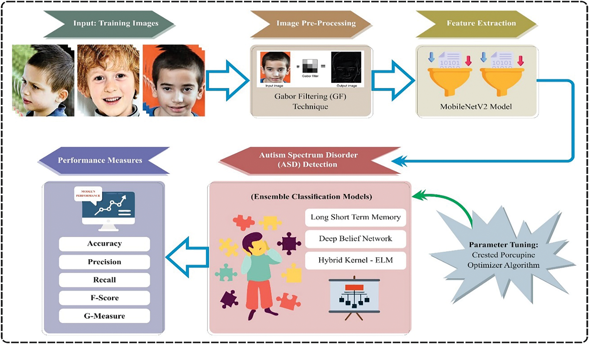
Figure 1: Overall flow of EDLM-ASDDFI model

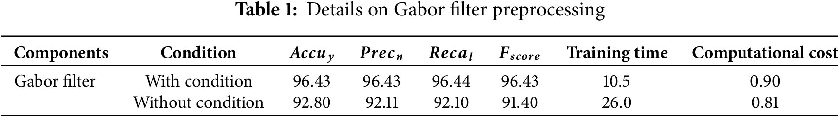
At a primary level, the EDLM-ASDDFI method undergoes data pre-processing, which is involved by GF. GF are linear filters that have been proposed to depict the sensitive field property of simple cells. Gabor filters are esteemed as very efficient instruments for feature extraction, especially in image-related applications like face recognition and pattern detection. These filters are derived from the visual processing functions of basic cells in the primary visual cortex of the brain. Their capacity to collect both spatial frequency (texture) and direction makes them particularly adept at augmenting and evaluating face pictures. Gabor filters extract orientation and frequency characteristics by identifying edges, contours, and textures across many orientations and scales (Table 1). This renders them especially effective at discerning the intricate details of face characteristics, including the eyes, nose, and mouth, which are essential for tasks such as recognition or classification. This filter can capture both the orientation and frequency data existing in the images. Enhancing face images by reducing the noise with Gabor filtering emphasizes spatial frequency components that correlate to face patterns to reduce irrelevant noise and enhance facial shapes and textures. Multi-scale and Multi-Orientation Analysis with Gabor filters of varied orientations and scales convolve input pictures to catch intricate patterns that change in direction and size. This multiple scales method enhances macro- and micro-facial traits. Preservation of Localized traits with the Gabor filter’s Gaussian envelope enables it to concentrate on particular picture areas, retaining wrinkles, expressions, and other minor traits needed for proper face analysis. The nose and mouth are essential for identification and categorization. These filter reactions have been gained in convolving imageries including GF of diverse orientations and scales. GF are normally described in the spatial domain, then they can also be identified in the domain of frequency. They are categorized by dual key parameters such as the orientation and the spatial frequency. This spatial frequency characterizes the number of oscillations or cycles from the filter along a known direction, and the orientation denotes the angle of the filter regarding the horizontal axis. The GF is mathematically described as the Gaussian function product and a composite sinusoidal function in Eq. (1):

G(x,y)=exp⁡(−x2+y22σ2)×exp⁡(J2πfx)(1)

whereas x and y denote the spatial coordinates, 0 is the standard deviation of the Gaussian function, f is the spatial frequency on the sinusoidal function, and j is the imaginary unit. Gabor filtering is distinctive compared to other models due to its robustness against variations in lighting and shading, prevalent challenges in facial image processing. Gabor filters emulate the receptive fields of neurons in the human visual system, rendering them particularly effective for applications involving human imagery, such as faces. Furthermore, Gabor filters yield rich localized features by integrating spatial and frequency information, which are essential for advanced tasks like facial recognition and emotion detection.

2.1 Feature Extractor: MobileNetV2

MobileNetV2 is a lightweight and efficient CNN architecture designed for mobile and embedded applications. It utilises depth-wise separable convolutions, inverted residuals, and linear bottlenecks to provide enhanced performance while reducing computational costs. The principal Attributes of MobileNetV2 are depth-wise separable convolutions, which decrease parameter count and computational cost by dividing convolution into depth-wise and pointwise processes. Inverted residuals facilitate effective feature reutilization by enlarging the input channels in the centre of the block and then reducing them to a smaller size. Linear bottleneck mitigates information loss by using linear activation instead of rectified linear unit (ReLU) after the bottleneck.

The EDLM-ASDDFI technique applies the MobileNetV2 model to learn complex features from the pre-processed data. To need mobile AI applications, Google has presented MobileNetV1, a lightweight CNN for embedded systems and mobile devices. Even with this, the performance and computational efficiency of MobileNetV1 can be improved. Therefore, Google presented MobileNetV2, which improves on MobileNetVl. When equated with MobileNetV1, MobileNetV2 presents Point-wise Convolution before Depth-wise Separable Convolution to effectively regulate feature channels. The 2nd pointwise convolution activation function was removed, whereas MobileNetV2, enchanting stimulation from the ResNet method, executed a short circuit link to reduce the calculations and parameters, thus improving the method’s performance. MobileNetV2 implements the reverse residual structure, initial increasing dimension, convolution, and then decreasing dimension. Utilize Shortcut connection when the output and input forms are similar and the size of the step is 1. Its deep separable structure of convolutional network mostly contains decreasing the number of parameters and computation. Generally, MobileNetV2 utilizes a light-weight NN (neural network) structure with lower method computational and complexity effort, utilizes residual connections to create the network steadier, unites more simply in training, and contains faster running speed and high accuracy, while upholding a size of method and memory footprint, which is appropriate for a range of hardware platforms like embedded and mobile devices. The input layer takes in red, green and blue (RGB) pictures with a resolution of 224 × 224 pixels. MobileNetV2 derives advanced characteristics from the input photos. The feature transformation layer prepares the feature vector for the ensemble classifiers. Ensemble classifiers, such as long short-term memory (LSTM), capture sequential dependencies. Deep belief networks (DBN) acquire hierarchical properties. Hybrid kernel extreme learning machine (HKELM) effectively classifies in high-dimensional spaces. The decision fusion layer integrates predictions via weighted voting or meta-classification. Final categorization judgment of the output layer.

2.2 ASD Detection Using Ensemble Learning

For the ASD detection process, the EDLM-ASDDFI method uses ensemble techniques for the classification procedure that encompasses LSTM, DBN, and HKELM. LSTM presented an inspiring work, which represents a superior iteration of recurrent neural networks (RNNs), exactly made to grab the general problem of long-term dependencies. Recognized to excel in holding data over protracted series, LSTM challenges the issue of vanishing gradient efficiently. The LSTM system processes the output of the previous time step and the input of the current time step at a hypothetical time step, so that the output is guided to the subsequent time step. The latter time-step and last hidden layer (HL) were generally employed for identification. The LSTM structure contains a memory unit that is symbolized by c, a HL signified by h, and 3 different gates such as input (i), forget (f), and output (o). All these gates play a vital part in managing the data movement out and into the memory unit, which efficiently handles writing and reading processes in the LSTM structure. Particularly, the input gate defines the method in which the internal state is upgraded depending upon the previous internal state and the present input. On the other hand, the forget gate rules the grade to where the preceding internal layer was kept. Finally, the output gate controls the effect of the internal layer on the complete method. More exactly, at every time-step t, the LSTM first gets an input xt. Besides the preceding HL ht−1. Then, it computes initiations for the gates and continues to upgrade both the HL to ht and the memory unit to ct. The mathematical procedure is defined below:

it=σ(Wxixt+Whiht−1+bi)(2)

ft=σ(Wxfxt+Whfht−1+bf)(3)

ct=ft⊙ct−1+it⊙tanh(Wxcxt+Whcht−1+bc)(4)

ot=σ(Wxoxt+Whoht−1+bo)(5)

ht=ot⊙tanh(ct)(6)

whereas σ(x) signifies the logistic sigmoid function, which is expressed as σ(x) = 1/(1 + exp(−x)). ⊙ represents the point-wise product process. b and W resemble the biases and weights linked with the memory unit and 3 gates.

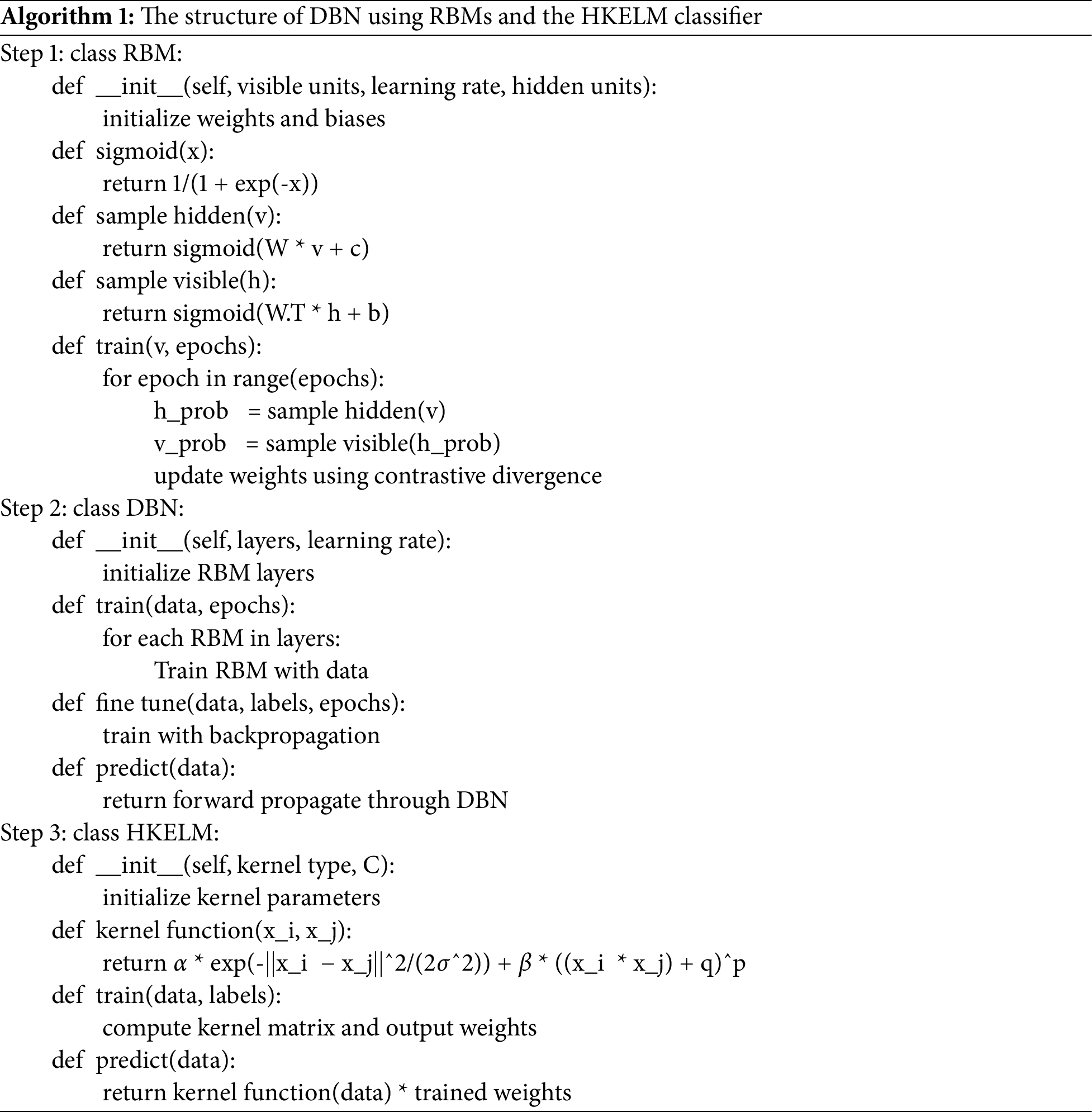
DBN is formed as a set of restricted Boltzmann machines (RBM). It contains dual layers such as a hidden layer (HL) neuron and a visible layer (VL) neuron. Particularly, there are no straight links among neurons within the same layer. As an alternative, RBMs are independent of one another, generalizing the assessment of predictable values for the measured variable. In a RBM, there is single HL and HL. RBMs are experts at absorbing the basic data structure and are mainly effective for tasks like dimensionality reduction and feature learning. They can accomplish the fundamental pattern in the data, which is beneficial for modules in DL structures like DBN in Algorithm 1. The formulation for the energy function is assumed in Eq. (7):

E(v,h)=−∑i=1n∑j=1mWijhivj−∑j=1mbjvj−∑i=1ncihi(7)

here, W represents the weight among HL and VL, and v and h refer to the input VL and HL, respectively. The bias value of every VL is b and HL is m. Whereas h and v are equivalent. The conditional probability densities of v and h.

P(v,h)=e−E(v,h)∑v,h′e−E(v,h′)(8)

P(B|A)=P(AB)P(A)(9)

p(hi=1|v)=sigmoid(∑j=1mWijvj+Ci)(10)

p(vi=1|h)=sigmoid(∑i=1nWijhi+bi)(11)

RBM utilizes the divergence of Kullback-Leibler to discover the dissimilarity between RBM and real distributions. It resolves the highest probability of the output layer as below:

L(θ)=∏i=1np(vi;θ),θ∈Θ(12)

By concluding it, we acquire the gradient of the RBM network:

∂ln⁡p(v)∂wij=vjp(hi=1|v)−1l∑k=1lvkp(hi=1|vk)(13)

∂lnp(v)∂bj=vj−1l∑k=1lvykj(14)

∂ln⁡p(v)∂ci=p(hi=1v)−1l∑k=1lp(hi=1vykj)(15)

Then, the RBM repeats these steps for weight offsets and updating.

KELM is a single HL feedforward neural network (NN) depending upon kernel function, the output of the feedforward NN method is attained by the below-given formulation:

f(x)=h(x)β=Hβ(16)

whereas y = f(x) denotes the network output, h(x) represents the input function of HL, x means the input vector, H refers to the matrix of feature mapping, β indicates the output of the weight vector involving the HL and the output layer. The influential non-linear mapping capability of the kernel function overwhelms the issue of random selection on parameters for KELM and enhances the capability to prolong the method. The KELM output function is stated below:

y(x)=h(x)β=h(x)HT(IC+HHT)−1T(17)

{HHT=ΩKELMΩKELMi,j=h(xi)h(xj)=K(xi,xj)(18)

while I denotes the unit matrix, C means penalty parameter, and Ω_KELM refers to the kernel function. Hence, the KELM model function formulation is given below:

y(x)=[K(x,x1)⋮K(x,xN)](IC+ΩKELM)−1T(19)

To efficiently enhance the capability that local and global search of the kernel function, a model of making a hybrid kernel function by the weight of linear is projected to get the HKELM, whose kernel function has the subsequent calculation:

{K(x,xj)=α⋅exp⁡(−‖x,xi‖22σ2)+β⋅((x⋅xj)+q)pβ=1−α,α∈[0,1](20)

here, 2σ2 denotes the parameter utilized to control the range of radial, p, and q represent exponential and constant parameters of the polynomial kernel function, correspondingly, α refers to the weight coefficient.

2.3 Optimization Model: CPO

Finally, the hyperparameter selection of the three DL models can be implemented by the design of the CPO technique. The CPO is a novel meta-heuristic method that emulates the defensive behaviour of crested porcupines for parameter optimization. Crested porcupines use four distinct defensive strategies visual, olfactory, physical, and auditory, when confronted with threats, depending on the nature of the assault. It offers novel insights and methodologies for research in pertinent fields. Establish the parameters N^′ T_max, α, T_f, T, and N_min as a random initialization of the population. If t < τ_max, evaluate the fitness value of the candidate solution to identify the optimal solution. Updating the Eq. (21) for the factor of defence γ_t.

γt=2×rand×(1−ttmax)ttmax(21)

Updating the population dimension with mathematical standard Eq. (22) for the cyclic population lessening techniques dynamically controls the population’s size to improve computational efficiency and maintain diversity.

N=Nmin+(N′−Nmin)×(1−(t% TmaxTTmaxT))(22)

whereas N′ represents the size of the population, α represents the speed factor of convergence, τ_f ∈ (0, 1) represents a pre-defined continuously balanced local exploitation (3rd protection method) and global exploitation (4th defence method), T represents a variable that determines cycle counts, t indicates the present function evaluation, τ_max means the maximum function count evaluations, % means the modulus or remainder operator, and N_(min) signifies the least individual counts in the recently made population; hence, the population size can’t be lower than N_min. This process diminishes population growth over time, mirroring the behaviour of crested porcupines, who activate defensive strategies just when faced with immediate danger, saving energy and resources. If i ∈ (0, 1), updating S and δ denotes the dual randomly generated values τ_8 and τ_9, when τ_8 < τ_9, insert the search level and create binary randomly formed integers τ_6 and τ_7, if τ_6 < τ_7, engage the 1st defence method, Articulate how people (candidate solutions) traverse the solution space contingent upon the adopted defensive technique promotes exploration by transitioning the solution towards a stochastically weighted amalgamation of the optimal solution and a random solution (Eq. (23)); or else, participate in the 2nd defence which navigates the search space by adjusting the answer according to the disparities among other candidates (Eq. (24)). When τ_8 > τ_9, consider the enlargement level, and stimulate a randomly generated value τ_10, if, τ_10 < T_f, involve the 3rd defence method enhances the search by concentrating on proximate options, emulating physical defence as porcupines confront local predators (Eq. (25)); or else, employ the 4th defence method focuses on exploiting the best-known solutions, refining them further to achieve optimal results (Eq. (26)). Iterating across t for obtaining the best fitness value of global, till t = T_max.

xi⟶t+1=xi⟶t+τ1×→|2×τ2×xCP⟶t−yi⟶t|(23)

xi⟶t+1=(1−U→1)×xi⟶t+U→1(y→+τ3×(xr1⟶t−xr2⟶t))(24)

xi⟶t+1=(1−U→1)×xi⟶t+U→1×(xr1⟶t+Sit×(xr2⟶t−xr3⟶t)−τ3×δ→×γt×Sit)(25)

xi⟶t+1=xCP⟶t+(α(1−τ4)+τ4)×(δ×xCP⟶t−xi⟶t)−τ5×δ×γt×Fi⟶t(26)

where xCP⟶t denotes the finest solution attained and characterizes CP, yi⟶t denotes the vector produced amongst the present CP and chosen at random CP from the population of predator position at t-th iteration, U→1 denotes a dual vector inside the interval of [0, 1], Sit denotes the trace factor of diffusion, δ→ denotes a parameter applied for controlling the search route, τi denotes a randomly generated value in [0, 1], xi⟶t denotes the location of the i-th individual at t-th iteration and similarly characterizes the hunter for location, Fi⟶t denotes the average power that affects the i-th hunter’s CP, and ri denotes a randomly formed value in [1, N]. Crested Porcupine Optimizer (CPO) fine-tunes hyperparameters and compares with and without CPO performance mode. The CPO approach acquires a feature function to get improved classification performance. A positive integer is defined to represent the optimal performances of the candidate solutions. This study investigates the decrease in the categorization error rate as shown in Eq. (27). The fitness function evaluates the quality of each response. Hyperparameter tweaking reduces the classification error rate, ensuring that the algorithm emphasizes hyperparameters that improve model accuracy.

fitness(xi)=ClassifierErrorRate(xi)(27)

The Crested Porcupine Optimizer (CPO) was selected for hyperparameter optimization because of its bio-inspired methodology, which emulates the foraging behaviour of porcupines. The Chief Product Officer adeptly balances research and exploitation, essential for traversing intricate hyperparameter search domains. In contrast to conventional techniques such as grid search or random search, CPO adeptly investigates favourable areas while circumventing early convergence to local optima. Its adaptive search technique, modelled after the porcupine’s defensive defences, facilitates quick convergence to optimum hyperparameter configurations. This results in enhanced model performance with diminished computational expense relative to less advanced optimization approaches.

3  Experimental Results and Analysis

In this section, the experimental validation analysis of the EDLM-ASDDFI algorithm is examined using the Autism image dataset, which comprises 2926 facial samples with two classes (Normal and Autism) as denoted. Regarding preprocessing, used Z-score normalization for colour normalization across all channels in standardizing pixel values. The image resizing dimensions (X, Y pixels) and the bicubic interpolation method were used. All preprocessing steps, including face detection using MTCNN (Multi-task convolutional neural network), and noise reduction using a median filter. For class imbalance, class weights were assigned inversely proportional to class frequencies. Elaborated on the potential impact of class imbalance on model training and class weighting was preferred over other techniques like oversampling or under-sampling due to limited data, oversampling could lead to overfitting. Data augmentation strategy random rotations between −15 and 15 degrees, horizontal flips, random cropping up to 10% of the image, and brightness adjustments between 0.8 and 1.2. The rationale behind choosing these augmentations emphasizes their role in preventing overfitting and introducing invariance to common image variations.

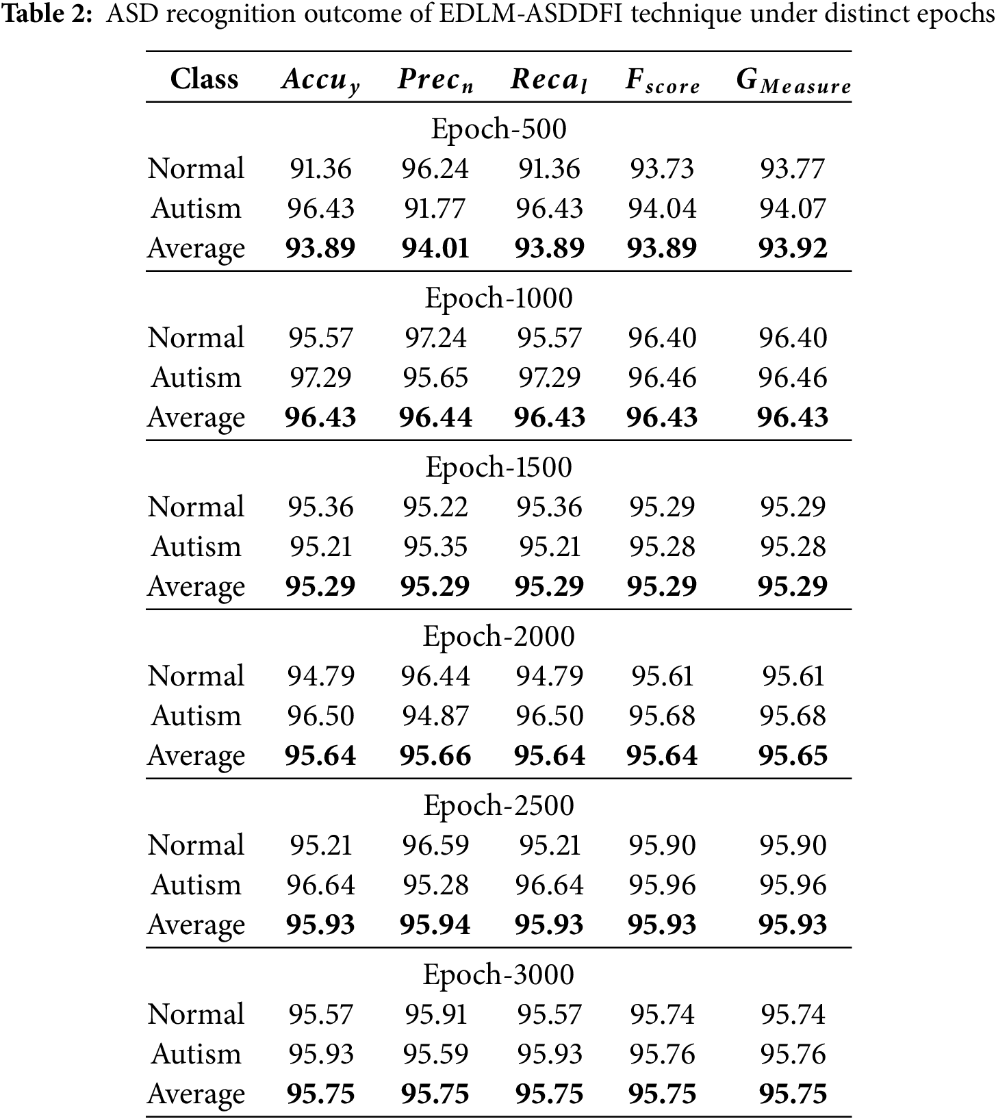
Reports a group of confusion matrices made by the EDLM-ASDDFI techniques on diverse epoch counts. On 500 epoch counts, the EDLM-ASDDFI approach has recognized 1279 samples as normal and 1350 samples as autism. Also, on 1000 epoch counts, the EDLM-ASDDFI models have recognized 1338 samples as normal and 1362 samples as autism. Succeeded by, on 1500 epochs, the EDLM-ASDDFI system has recognized 1335 samples as normal and 1333 samples as autism. Moreover, on 2000 epoch counts, the EDLM-ASDDFI methods have recognized 1327 samples as normal and 1351 samples as autism. The collection intends to classify images of the faces of autistic children, perhaps facilitating early identification and analysis. The dataset seeks to distinguish these based on face characteristics, suggesting a possible class imbalance that requires consideration. Processing problems include class imbalance; when the quantity of pictures in one class (e.g., Non-Autistic) substantially exceeds that of another class (e.g., Autistic), it may result in biased model performance. Consequently, class weighting was introduced during model training. Colour normalization was done during preprocessing to reduce noise. The ASD recognition results of the EDLM-ASDDFI approach are defined under different epoch counts. On 500 epoch counts, the EDLM-ASDDFI methods offer an average accu_y of 93.89%, prec_n of 94.01%, reca_l of 93.89%, F_score of 93.89%, and G_Measure of 93.92%. Also, on 1000 epochs, the EDLM-ASDDFI models present an average accu_y of 96.43%, prec_n of 96.44%, reca_l of 96.43%, F_score of 96.43%, and G_Measure of 96.43%. In the meantime, on 2000 epoch counts, the EDLM-ASDDFI methodology offers an average accu_y of 95.64%, prec_n of 95.66%, reca_l of 95.64%, F_score of 95.64%, and G_Measure of 95.65%.

Additionally, on 3000 epoch counts, the EDLM-ASDDFI approach presents an average accu_y of 95.75%, prec_n of 95.75%, reca_l of 95.75%, F_score of 95.75%, and G_Measure of 95.75%. Providing a performance measure that strikes a compromise between recall and accuracy, which is crucial in datasets with unequal class distribution. Without the need for a set threshold, the receiver operating characteristic area under the curve (ROC-AUC) provides information about the classifier’s overall performance and assesses its capacity to differentiate between the two classes (Autistic and Normal). Precision shows the proportion of real positive cases (Autistic) that match the expected positive cases. Crucial for reducing false positives. The number of accurately detected genuine positives (autistic) is shown by the recall. Vital to guaranteeing the detection of every instance of autism. Researchers evaluated the suggested model’s comparative performance by contrasting it with the most advanced methods in the field, paying particular attention to accuracy, resilience, and computing efficiency under various experimental conditions. Comparative metrics based on accuracy demonstrate the degree to which the model can categorize data. Recall and accuracy are balanced by the F1-Score, which is essential for unbalanced datasets.

ROC-AUC assesses how well the classifier can differentiate across classes. Computational time, which is important for real-time applications, quantifies how long it takes the model to make an inference. Performance is evaluated for robustness in the presence of noise, occlusion, and illumination fluctuations. In Comparative Analysis, the computational efficiency of the suggested model (EDLM-ASDDFI) surpasses other approaches, requiring just 0.85 s for inference. Lightweight solutions such as MobileNet exhibit increased speed (1.10 s) at the expense of accuracy and resilience. Techniques using VGG-16 architecture (e.g., Logistic Regression, Random Forest) exhibit prolonged inference durations (4.65–5.20 s), rendering them less appropriate for real-time applications. Robustness assessments demonstrate that EDLM-ASDDFI has an accuracy decline of less than 2% with noise addition, while other approaches exhibit declines of 4–8%. MobileNet, despite its computational efficiency, exhibits considerable performance decline in noisy situations, indicating limited resilience. The accuracy of the proposed model attains the maximum accuracy at 96.43%, surpassing MobileNet at 90.24% and VGG-16-based methods, which range from 89.55% to 92.64%. Gradient Boosting achieves a performance of 92.64%, although it underperforms in recall and F1-score because of its susceptibility to class imbalance.

The training and validation accuracy results of the EDLM-ASDDFI method across various epoch counts. The accuracy values are calculated for epoch counts ranging from 0 to 3000. This figure highlighted that the training and validation accuracy values exhibit an upward trend, indicating the efficacy of the EDLM-ASDDFI approaches throughout several rounds. Furthermore, the training and validation accuracies remain closely aligned throughout the epoch counts, indicating less overfitting and enhanced performance of the EDLM-ASDDFI system, hence ensuring consistent predictions on unseen data. The training and validation loss curve of the EDLM-ASDDFI approach over varying epoch counts. The loss values are calculated for epoch counts ranging from 0 to 3000. The training and validation accuracy values indicate a declining trend, reflecting the EDLM-ASDDFI approach’s capacity to manage the trade-off between generalization and data fitting. The continual reduction in loss values indicates enhanced effectiveness of the EDLM-ASDDFI approach and optimizes prediction results over time. The precision-recall (PR) curve analysis of the EDLM-ASDDFI method over various epoch counts, illustrates its performance by graphing Precision vs. recall for each class label. This figure illustrates that the EDLM-ASDDFI technique consistently achieved superior PR values across various classes, highlighting its ability to maintain a significant proportion of true positive predictions (precision) while also capturing a substantial number of actual positives (recall). The consistent increase in PR outcomes across all class labels illustrates the efficacy of the EDLM-ASDDFI method inside the categorization framework.

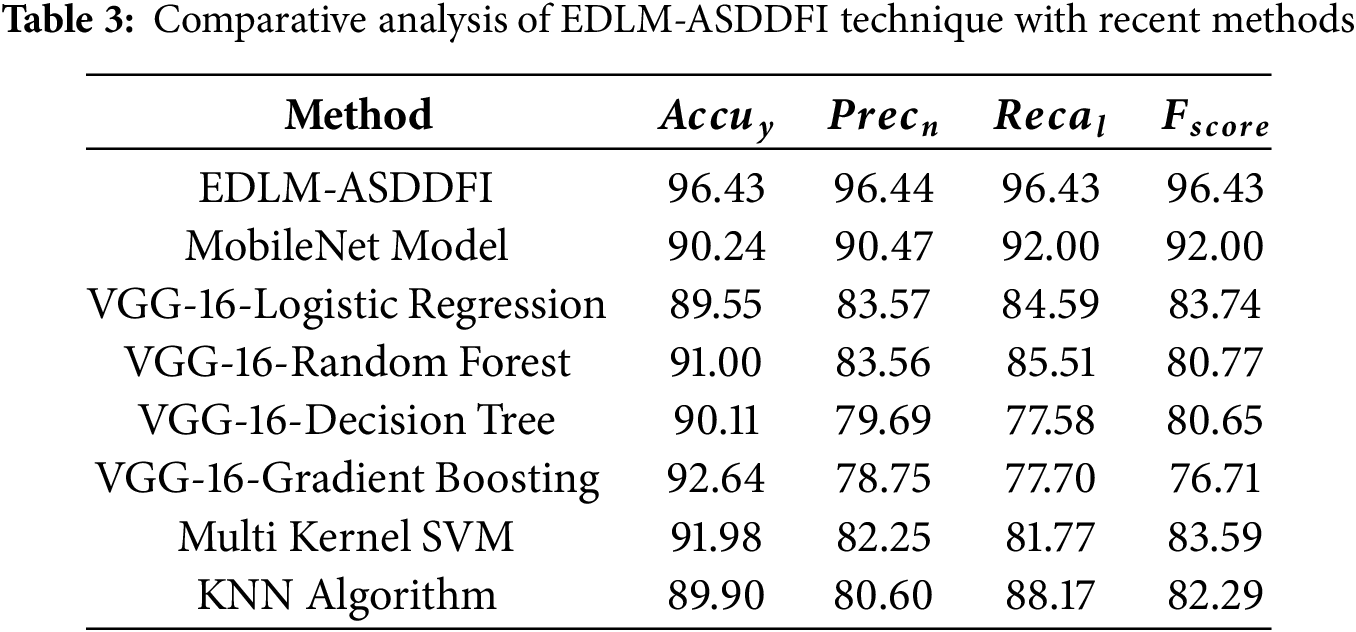
The ROC curve of the EDLM-ASDDFI system is considered. The outcomes suggest that the EDLM-ASDDFI method under separate epochs reaches boosted ROC outcomes over every class, indicating a major ability to discern the classes. This consistent trend of amended ROC values over several classes suggests the capable performance of the EDLM-ASDDFI method in forecasting classes, emphasizing the strong nature of the classification method. Table 2 proves the experimental outcomes of the EDLM-ASDDFI system are compared with existing works. On equating with accu_y, the EDLM-ASDDFI model shows its supremacy with an enlarged accu_y of 96.43% while the MobileNet, VGG-16-LR, VGG-16-RF, VGG-16-DT, VGG-16-GB, Multi Kernel SVM, and KNN (K-Nearest Neighbor) approaches get reduced performance with accu_y of 90.24%, 89.55%, 91.00%, 90.11%, 92.64%, 91.98%, and 89.90%, respectively. Moreover, equating with F_score, the EDLM-ASDDFI system shows its power with an improved F_score of 96.43% where the MobileNet, VGG-16-LR, VGG-16-RF, VGG-16-DT, VGG-16-GB, Multi Kernel SVM, and KNN approaches get reduced performance with F_score of 92.00%, 83.74%, 80.77%, 80.65%, 76.71%, 83.59%, and 82.29%, respectively.

To investigate the generalization capabilities of the proposed model (EDLM-ASDDFI), evaluate its performance on unseen data by cross-validation and a distinct benchmark dataset. Generalization is an essential attribute that guarantees the model’s efficacy on data outside its training set, making it robust and dependable for practical applications Table 3. Inevitably applied 5-fold cross-validation to evaluate the model’s capacity for generalization to novel data. The dataset was partitioned into five subsets, with each fold employing 80% of the data for training and 20% for testing. The model consistently attained elevated accuracy and F1 scores across all folds, exhibiting minimal variance. This stable performance signifies robust generalization on the specified dataset.

The comparative evaluation of classification models indicates that the EDLM-ASDDFI model obtains improved performance across accuracy, precision, recall, and F-score. The improvement is credited to the ensemble learning architecture, which utilizes many classifiers for superior decision-making, lowering bias and variation. Additionally, the incorporation of CPO-based parameter adjustment provides optimum hyperparameter selection, significantly enhancing model efficiency. MobileNetV2’s superior feature extraction capabilities help greatly to better ASD detection by collecting fine-grained face patterns. The proposed model’s superior performance, as shown in comparative results, highlights its robustness in feature representation and classification, making it a more reliable approach for ASD identification compared to traditional methods. In Table 4, the comparative outcomes of the EDLM-ASDDFI system are stated in terms of computational time (CT). The results recommend that the EDLM-ASDDFI technique obtains improved performance. Based on CT, the EDLM-ASDDFI approach gets a reduced CT of 0.94 s while the Mobile-Net, VGG-16-LR, VGG-16-RF, VGG-16-DT, VGG-16-GB, Multi Kernel SVM, and KNN methodologies achieve higher CT values of 2.55, 4.45, 4.24, 4.18, 4.59, 3.95, and 4.53 s, respectively, in Fig. 2.

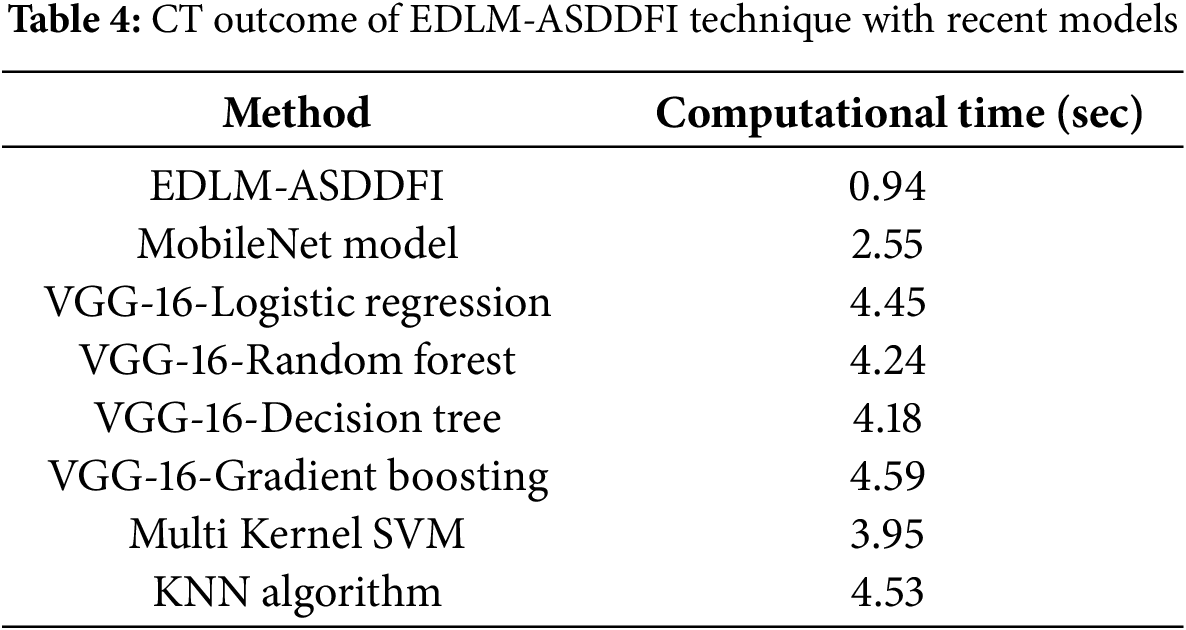
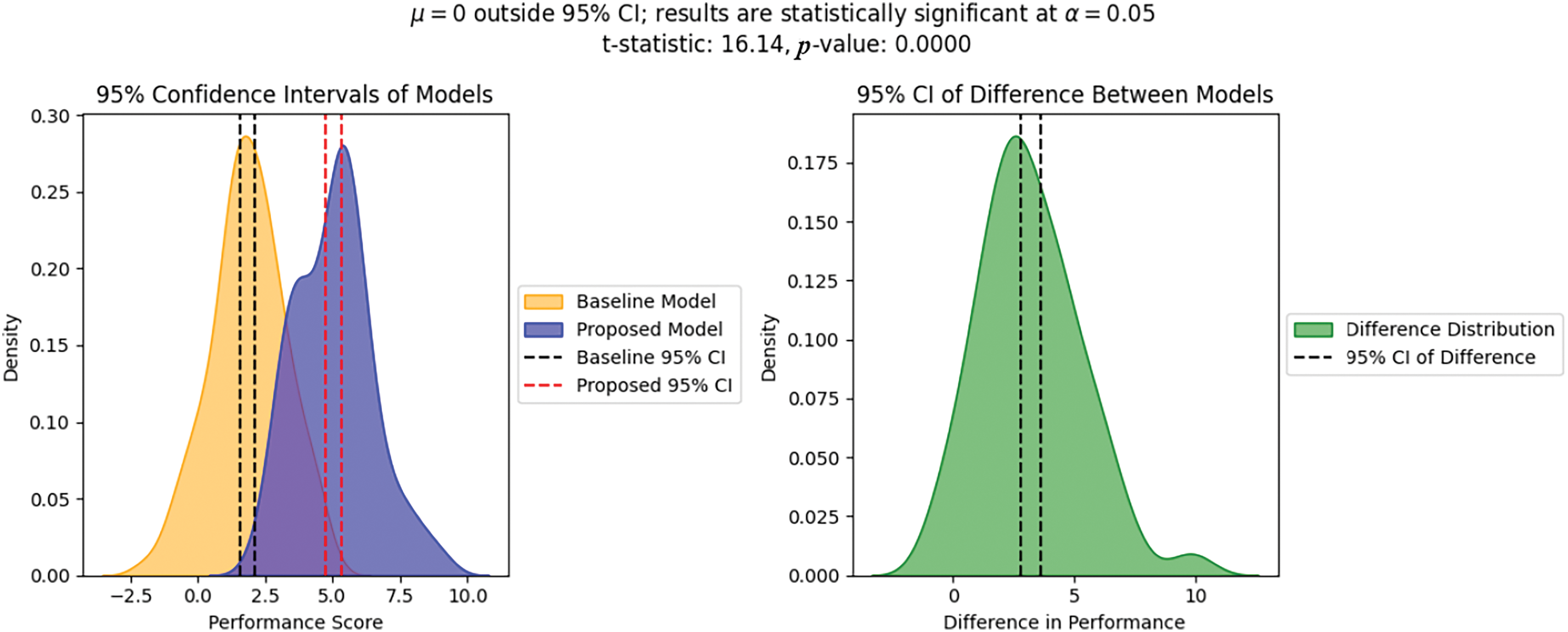
Figure 2: CT outcome confidence interval of models with statistically significant

4  Conclusion

In this study, we have developed an EDLM-ASDDFI model. The main objective of the EDLM-ASDDFI model is to recognize the dissimilar stages of ASD employing facial images. In the EDLM-ASDDFI method, the primary level of data pre-processing is involved by GF. Besides, the EDLM-ASDDFI technique applies the MobileNetV2 model to learn complex features from the pre-processed data. For the ASD detection process, the EDLM-ASDDFI method uses ensemble techniques for the classification procedure that encompasses LSTM, DBN, and HKELM. Finally, the hyper-parameter selection of the three DL classifiers is implemented by the design of the CPO system. An extensive experiment was conducted to emphasize the improved ASD detection performance of the EDLM-ASDDFI method. The simulation outcomes indicated that the EDLM-ASDDFI technique highlighted betterment over other existing models in terms of numerous performance measures. Augmenting the dataset by an increase in size and variety may enhance statistical dependability. Augmenting the dataset with superior feature representations might enhance insight approaches like as SIFT (Scale Invariant Feature Transform), HOG (Histogram of Oriented Gradient), or CNN-based feature extraction. Multimodal learning enhances contextual insights for performance assessment by integrating image-based model performance measures with IoT sensor data from practical applications.

Acknowledgement: The authors extend their appreciation to King Saud University for funding the publication of this research through the Researchers Supporting Grant Project number (RSPD2025R1107) by King Saud University, Riyadh, Saudi Arabia.

Funding Statement: Researchers supporting Project number (RSPD2025R1107), King Saud University, Riyadh, Saudi Arabia.

Author Contributions: Conceptualization, Mohammad Zakariah and Jagadesh Balasubramani; methodology, Surendran Rajendran; software, Jagadesh Balasubramani; validation, Surendran Rajendran and Jagadesh Balasubramani; formal analysis, Mohammad Zakariah; investigation, Surendran Rajendran; resources, Mohammad Zakariah; data curation, Abeer Alnuaim; writing—original draft preparation, Surendran Rajendran; writing—review and editing, Surendran Rajendran; visualization, Abeer Alnuaim; supervision, Abeer Alnuaim; project administration, Surendran Rajendran; funding acquisition, Abeer Alnuaim and Mohammad Zakariah. All authors reviewed the results and approved the final version of the manuscript.

Availability of Data and Materials: Openly available in the Kaggle repository at https://www.kaggle.com/datasets/cihan063/autism-image-data (accessed on 22 November 2024).

Ethics Approval: This study did not involve direct experiments on humans or the use of human tissue samples. Instead, publicly available datasets were utilized specifically datasets from Kaggle.

Conflicts of Interest: The authors declare no conflicts of interest to report regarding the present study.

References

1. Nogay HS, Adeli H. Machine learning (ML) for the diagnosis of autism spectrum disorder (ASD) using brain imaging. Rev Neurosci. 2020;31(8):825–41. doi:10.1515/revneuro-2020-0043. [Google Scholar] [PubMed] [CrossRef]

2. Liao M, Duan H, Wang G. Application of machine learning techniques to detect children with autism spectrum disorder. J Healthc Eng. 2022;22(1):9340027. doi:10.1155/2022/9340027. [Google Scholar] [PubMed] [CrossRef]

3. Yang X, Zhang N, Schrader P. A study of brain networks for autism spectrum disorder classification using resting-state functional connectivity. Mach Learn Appl. 2022;8(164):100290. doi:10.1016/j.mlwa.2022.100290. [Google Scholar] [CrossRef]

4. Ibadi H, Lakizadeh A. ASDvit: enhancing autism spectrum disorder classification using vision transformer models based on static facial features images. Intell-Based Med. 2025;11(11):10026. doi:10.1016/j.ibmed.2025.100226. [Google Scholar] [CrossRef]

5. Raj S, Masood S. Analysis and detection of autism spectrum disorder using machine learning techniques. Procedia Comput Sci. 2020;167(12):994–1004. doi:10.1016/j.procs.2020.03.399. [Google Scholar] [CrossRef]

6. Bhola J, Jeet R, Jawarneh MMM, Pattekari SA. Machine learning techniques for analysing and identifying autism spectrum disorder. In: Kautish S, Dhiman G, editors. Artificial intelligence for accurate analysis and detection of autism spectrum disorder. Hershey, PA, USA: Global; 2021. p. 69–81. [Google Scholar]

7. Rahman M, Usman OL, Muniyandi RC, Sahran S, Mohamed S, Razak RA. A review of machine learning methods of feature selection and classification for autism spectrum disorder. Brain Sci. 2020;10(12):949. doi:10.3390/brainsci10120949. [Google Scholar] [PubMed] [CrossRef]

8. Alhakbani N. Facial emotion recognition-based engagement detection in autism spectrum disorder. Int J Adv Comput Sci Appl. 2024;15(3):1–27. [Google Scholar]

9. Thanarajan T, Alotaibi Y, Rajendran S, Nagappan K. Eye-tracking based autism spectrum disorder diagnosis using chaotic butterfly optimization with deep learning model. Comput Mater Contin. 2023;76(2):1995–2013. doi:10.32604/cmc.2023.039644. [Google Scholar] [CrossRef]

10. Sharma A, Tanwar P. Autism spectrum disorder prediction system using machine learning and deep learning. Int J Appl Syst Stud. 2024;11(2):159–73. doi:10.1504/IJASS.2024.140025. [Google Scholar] [CrossRef]

11. Khan B, Bhatti SM, Akram A. Autism spectrum disorder detection in children via deep learning models based on facial images. Bull Bus Econ. 2024;13(1):1–27. doi:10.61506/01.00241. [Google Scholar] [CrossRef]

12. Vidyadhari C, Karrothu A, Manickavasagam P, Anjali Devi S. Autism spectrum disorder detection using fractional social driving training-based optimization enabled deep learning. Multimed Tools Appl. 2024;83(13):37523–48. doi:10.1007/s11042-023-16784-x. [Google Scholar] [CrossRef]

13. Alkahtani H, Aldhyani TH, Alzahrani MY. Deep learning algorithms to identify autism spectrum disorder in children-based facial landmarks. Appl Sci. 2023;13(8):4855. doi:10.3390/app13084855. [Google Scholar] [CrossRef]

14. Gaddala LK, Kodepogu KR, Surekha Y, Tejaswi M, Ameesha K, Kollapalli LS, et al. Autism spectrum disorder detection using facial images and deep convolutional neural networks. Rev D’intelligence Artif. 2023;37(3):1–18. doi:10.18280/ria.370329. [Google Scholar] [CrossRef]

15. Umanandhini D. Deep learning algorithms for children-based facial expression to recognize autism spectrum disorder. J Nonlinear Anal Optim. 2023;14(2):1906–9685. [Google Scholar]