TRLLD: Load Level Detection Algorithm Based on Threshold Recognition for Load Time Series

1  Introduction

Load time series, also referred to as time series load flow (TLF), refers to the resource consumption data recorded over specific time intervals [1], such as cloud computing resource loads, website and database access volumes, or electricity consumption. In the context of the rapid development of the internet, cloud computing, and engineering management, massive amounts of load time series data are continuously generated across various fields. As an important and complex data object, load time series accurately captures valuable information about applications and plays a crucial role in different domains. By analyzing the characteristics of load time series, it is possible to perform anomaly detection, optimize real-time resource allocation strategies, or forecast future loads [2].

Despite the significant applications of load time series analysis across various fields, there exist notable gaps in the current research within this domain. Firstly, existing studies primarily focus on identifying extreme points such as peaks and troughs in load time series. However, the classification of load levels often relies not only on these extremes but also on the overall load variation within specific time intervals [3,4]. Therefore, it is essential to incorporate load level labeling data, normalized load values at different load levels, and load rates [5] into the analysis. Secondly, the current research generally lacks a dynamic description of load levels, often employing simple fixed thresholds for classification, which limits sensitivity and adaptability to load variations. Simple fixed thresholds may fail to capture the subtle differences in load variations, leading to incorrect load classification. Lastly, while load time series are widely applicable across different fields and scenarios, there are substantial numerical differences between various datasets [6,7], and a standardized perspective independent of specific values is lacking to assess the characteristics of load time series across different domains. Addressing these gaps will provide researchers with effective tools to quickly evaluate the applicability of existing methods to specific load time series datasets.

The main contributions of this paper are summarized as follows:

a   A Threshold Recognition-based Load Level Detection Algorithm (TRLLD) has been implemented, characterized by non-parametric properties, low sample friendliness, low spatiotemporal complexity, and high robustness. The algorithm leverages the inherent features of the time series samples, enabling it to effectively identify high load level regions and low load level regions based on sample distribution density uniformity, ultimately yielding normalized load values to facilitate understanding of sample patterns and identification of anomalies. This distinguishes it from peak and trough detection methods, which focus solely on local data points, providing a holistic analytical perspective for load time series.

b   A Density Uniformity Index Based on Differences (DUID) and its computation method have been proposed, applied directly in this algorithm. The DUID uses samples with absolutely uniform distribution density as a reference, effectively representing the distribution density uniformity of load time series samples. When the sample distribution density is uneven, the algorithm sets a higher threshold to prevent noise interference; conversely, when the density is uniform, a lower threshold is set to capture more data features, enabling comprehensive identification of valid signals. Existing statistical measures of density uniformity, such as the chi-squared test, rely on fixed intervals to determine whether to reject the null hypothesis, which prevents automatic adjustment based on the actual distribution of the samples. Furthermore, the chi-squared test requires the construction of a frequency table and the calculation of statistics, which can increase computational complexity when handling large-scale data. In contrast, the DUID dynamically compares the density differences of reference samples, effectively reflecting distribution characteristics and enabling sample adaptivity.

c   The concepts of High Load Level Concentration (HLLC) and Low Load Level Concentration (LLLC) have been introduced, along with a statistical interpretation based on the algorithm described in this paper. HLLC and LLLC provide a standardized perspective independent of load values, allowing horizontal comparisons of load levels across different time periods and scenarios. They effectively explain load distribution characteristics, reflect relative differences in load levels, and indicate volatility within corresponding load level regions, serving as an important reference when load capacity limits are uncertain.

d   The proposed DUID was verified and confirmed to effectively reflect the uniformity of sample distribution density. The performance of the TRLLD algorithm was evaluated on both scene samples and synthetic samples to verify its broad applicability. The output features of the algorithm were confirmed by obtaining a 95% confidence interval through bootstrap sampling. Additionally, five additive noises of different intensities were introduced to confirm the algorithm’s high robustness.

2  Related Work

2.1 Load Time Series Analysis

Load time series analysis is a vital research area in various fields such as computer networks, cloud computing, information systems, and database management. In Management Systems Engineering, it is essential for optimizing performance, enhancing efficiency, and achieving intelligent management.

In computer networks and cloud computing, load time series analysis monitors network traffic and resource usage. Analyzing network load data helps optimize performance and address congestion issues. For example, Bhalaji used time series forecasting for workload allocation to improve network performance [8]. Yadav et al. applied LSTM deep learning for predicting server loads [9]. Khan et al. analyzed workload data as time series to identify virtual machine groups with similar patterns [10].

In information systems and database management, load time series analysis helps identify peak usage and access trends, optimizing storage and retrieval. Higginson et al. employed supervised machine learning to find patterns in workload time series for database capacity planning [11]. McDonald created large database workloads in a private cloud for time series forecasting in hybrid clouds [12].

In Management Systems Engineering, power systems and energy management are significant application areas [13]. Analyzing power load data with machine learning for forecasting is a mainstream direction. Motlagh et al. clustered residential electricity users using load time series for market segmentation [14]. Shilpa et al. proposed a stochastic model for short-term power load forecasting [15]. Loganathan et al. introduced deep learning-based forecasting for photovoltaic generation [16].

2.2 Load Level Detection

Load level detection involves identifying and classifying different load levels within time series data, primarily aiming to automate the recognition of high and low load regions through historical data analysis. This supports resource management and optimization decisions. While peak and trough detection is a key technique for identifying significant change points in load data, load level detection encompasses a broader analysis to classify multiple load intervals and describe load states comprehensively.

In peak and trough detection, peaks indicate high load states, and troughs indicate low load states, helping researchers respond to drastic load changes. For example, Palshikar proposed an algorithm for defining and detecting local peaks in time series to analyze significant events [17]. Schneider utilized statistical definitions based on geometric trends to detect peaks and troughs in time series [18]. Li et al. integrated peak and trough identification into Complex Event Processing (CEP) technology for detecting cloud computing system states [19]. Cao et al. used peak and trough identification to optimize cloud resource allocation in smart grid demand-side management [20].

Load level identification offers a broader perspective, focusing on in-depth analysis of load time series to determine characteristics and patterns across various scenarios. Gupta et al. reviewed early classification methods for time series, highlighting their importance in medical diagnosis and industrial monitoring for timely decision-making [21]. Tsekouras et al. explored pattern recognition methods for classifying load time series to analyze electricity consumption behavior more comprehensively [22]. Manojlović et al. proposed a grouping algorithm combining dimensionality reduction and clustering to identify similar load patterns, optimizing load data models in distribution utilities [23].

Rule-based methods in load level identification and classification exhibit strong interpretability and ease of understanding, allowing users to clearly comprehend the decision-making process of the model. These methods typically rely on expert knowledge and experience, using explicit rules to guide load classification, making them suitable for scenarios where rules are well-defined and subject to minimal change. For example, Qi et al. applied decision trees for identifying load patterns to classify customers into different clusters [24].

Machine learning methods also represent a major research trend in this field. Due to their ability to automatically learn features and patterns from data, they demonstrate greater adaptability and accuracy when handling complex and nonlinear load data. Tambunan et al. employed the K-Means clustering algorithm for analyzing electrical peak loads and provided load level ratings categorized as high, medium, and low [25]. Similarly, Rajabi et al. utilized clustering methods to extract latent patterns from energy consumption [26].

Existing load level detection methods often focus excessively on the detection of extreme points or merely serve as a means of pattern classification, lacking a comparative methodology. This narrow perspective hinders a comprehensive understanding of the complexity and dynamic changes of load data, resulting in difficulties in effectively supporting resource management and optimization decisions in practical applications.

2.3 Outlier Detection

In load time series analysis, outlier detection is crucial for identifying abnormal data points that deviate significantly from normal patterns. These outliers often indicate extreme load conditions due to system failures, sudden events, or other anomalies. While load level detection focuses on classifying load states, outlier detection aims to discover deviations from normal patterns, enabling timely interventions to mitigate negative impacts on system performance. Often, load level detection integrates outlier detection to minimize the influence of outliers on classification results, as outliers can represent extreme load levels and are important for resource management and decision support.

Researchers have developed various methods for effective outlier identification in load time series. The effectiveness of these methods varies significantly with different data distributions, making method selection crucial [27]. Classic outlier detection techniques include Z-score [28], IQR (Interquartile Range) [29], DBScan [30], Isolation Forest [31], and Random Forest [32]. Additionally, new methods have emerged. For instance, Almardeny et al. proposed a non-parametric anomaly detection method that constructs outlier scores by decomposing the attribute space and rotating data points, showing superior performance across datasets [33]. Boukerche et al. reviewed advancements in anomaly detection, analyzing the characteristics and future directions of emerging methods [34].

For time series data, Blázquez-García et al. reviewed the latest unsupervised anomaly detection techniques [35]. Zamanzadeh Darban et al. provided a systematic review of deep learning applications in time series anomaly detection, discussing various strategies and their strengths and weaknesses [36].

The application of outlier detection in load time series analysis has proven effective. Luo et al. proposed a real-time anomaly detection method using a dynamic regression model and adaptive thresholds, enhancing short-term load forecasting accuracy [37]. Yue et al. introduced a descriptive analysis-based method that improved network security load forecasting by increasing the true positive rate and reducing the false positive rate [38]. Cook et al. reviewed anomaly detection techniques in IoT time series data, discussing challenges and case studies [39].

For the subject of this paper, load level detection, directly using the results of outlier detection as the outcomes of load level detection may lead to a one-sided analysis, overlooking the fact that outliers are only a part of the load characteristics. Such a one-dimensional analytical approach may result in misjudgments regarding the load state, thereby affecting the effectiveness of resource management and decision support.

3  Algorithm Description

3.1 Algorithm Characteristics and Overview

Compared to directly using outlier detection, fixed thresholds, or quantile methods, the main characteristics of the TRLLD algorithm are as follows:

a   The TRLLD algorithm effectively identifies anomalies and peaks in load time series by incorporating outlier detection, thereby improving the accuracy and reliability of load level detection. The load time series data samples are flexible and variable, making it unreasonable to assume they follow any specific distribution type. The use of the IQR method is due to its non-parametric nature, which allows it to adapt to data of different distribution types, eliminating dependence on distribution assumptions. Therefore, using the IQR method to ensure the non-parametric characteristics of the TRLLD algorithm is justified. In contrast, the commonly used Z-score method and its modified version, the Modified Z-score, are parametric methods, and thus will not be adopted in the TRLLD algorithm. Compared to machine learning methods, the IQR method is faster in computation and does not require complex model training and tuning, making it suitable for real-time monitoring. This simple and intuitive approach is easy to understand and implement, making it applicable to various practical scenarios.

b   The algorithm enhances adaptability to different samples by introducing the Density Uniformity Index Based on Differences (DUID). DUID provides a quantitative metric by calculating the density differences between the input samples and the ideal uniform distribution samples, helping the algorithm identify the distribution characteristics of the samples. When the distribution density of the load time series is uneven, DUID prompts the algorithm to raise the threshold, thereby reducing noise interference from low-density areas and lowering the risk of misidentification.

c   HLLC and LLLC effectively represent the distribution characteristics of load time series. HLLC quantifies the concentration of data points within high load areas, with higher HLLC values indicating that the load is highly concentrated over a short period (e.g., 80% of the load concentrated in 20% of the time), which helps identify situations of resource abundance. Conversely, LLLC quantifies the concentration of data points in low load areas, with lower LLLC values indicating that low load areas occupy a small proportion but have a large time span (e.g., 20% of the load concentrated over 80% of the time), aiding in the identification of instances of resource idleness.

d   By standardizing results and providing statistical interpretations, the output becomes easier to understand. Furthermore, the introduction of reference load capacity allows the system to directly express resource utilization rates as percentages under different load levels, helping managers quickly identify areas of resource utilization and formulate appropriate resource allocation strategies.

The intuitive comparison is illustrated in Fig. 1. The TRLLD algorithm ensures the identification of high load level regions and low load level regions within any load time series. Furthermore, it demonstrates greater robustness in handling noise and outliers.

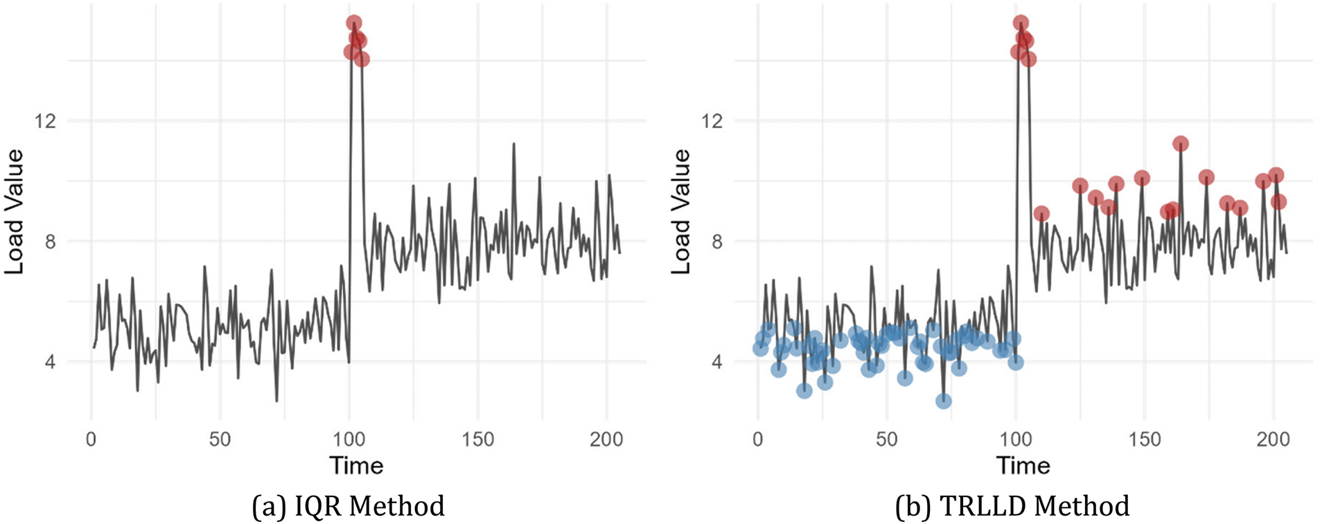
Figure 1: Load level detection: IQR vs. TRLLD

The TRLLD algorithm described in this paper takes load time series data, two control parameters, and a reference carrying capacity (CRef) as inputs. One of the control parameters is the IQR outlier detection threshold (TIQR), and the other control parameter is the algorithm sensitivity (α). The specific calculation process is as follows:

a   Use the IQR method to identify outliers in the load time series, resulting in an Outlier-Removed Time Series.

b   Utilize the DUID and its algorithm, as proposed in this paper, to determine the sample distribution density uniformity characteristics of the Outlier-Removed Time Series.

c   Calculate the high load level threshold and low load level threshold using the obtained DUID. Data points above the high load level threshold are classified as the High Load Level Region, while data points below the low load level threshold are classified as the Low Load Level Region.

d   Calculate the HLLC and LLLC for the High Load Level Region and Low Load Level Region, respectively.

e   Obtain the statistical interpretations of HLLC and LLLC, and output three normalized results expressed as percentages, in conjunction with the reference carrying capacity (CRef).

The overall process and operational mechanism of the TRLLD algorithm are illustrated in Fig. 2.

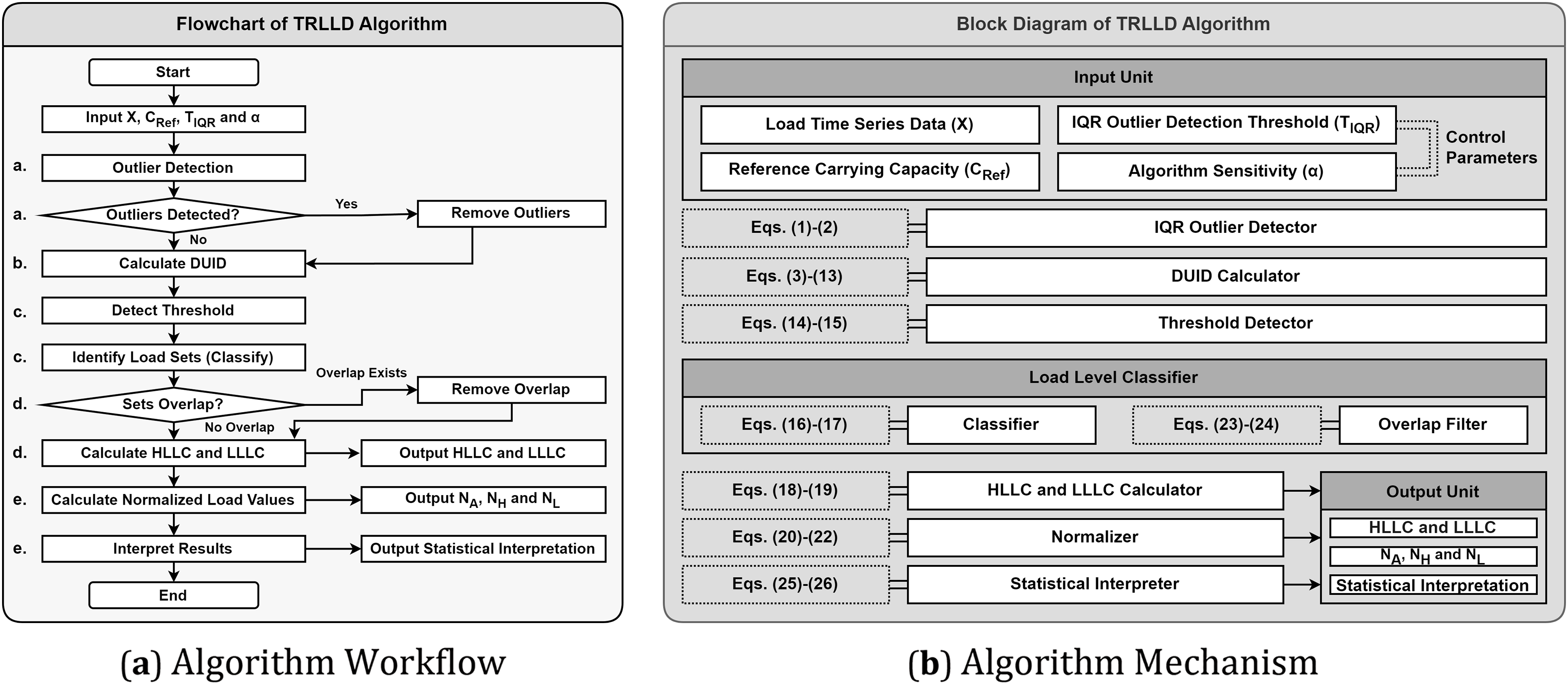
Figure 2: TRLLD algorithm overview

The flowchart Fig. 2a systematically presents the execution steps of the algorithm, clearly labeling the corresponding steps (a–e) as described in the preceding paragraphs, while emphasizing the logical sequence and decision points during the algorithm’s execution. The block diagram Fig. 2b provides an in-depth analysis of the algorithm’s components and implementation mechanisms, linking the equation numbers to the mathematical models and statistical interpretation processes in Sections 3.2 and 3.3. This offers a detailed perspective on the internal workings of the algorithm and establishes a clear framework and reference for subsequent optimization and application.

3.2 Mathematical Model of the Algorithm

In this section, we will provide a detailed description of the mathematical model of the TRLLD algorithm and its core computational processes. Overall, the algorithm is divided into four main parts: the first part involves obtaining the outlier-removed load time series; the second part calculates the DUID of the samples; the third part performs threshold recognition and obtains the sets of different load levels; and the final part calculates the HLLC and LLLC, normalizing the output based on the reference carrying capacity (CRef).

X, CRef, TIQR, and α are the input parameters for the algorithm.

The first part involves obtaining the outlier-removed load time series. We use the IQR outlier detection method to identify outliers in the input load time series. Since IQR is a common and effective outlier detection method, this paper will not provide a detailed explanation of its calculation process. Outliers are directly identified using the IQR method, resulting in the outlier set O, defined as follows:

O={xt∈X|xt<LB∨xt>UB}(1)

where X represents the input load time series and xt denotes a data point within that series. LB and UB represent the lower and upper limits for identifying outliers, respectively.

Then, the identified outliers are removed from the original load time series to obtain the outlier-removed load time series X′:

X′={xt∈X|xt∉O}={x1,x2,⋯,xm}(2)

where m is the length of the outlier-removed time series.

The second part is the key component of the algorithm, where we calculate the DUID for the load time series to quantify the distribution density uniformity of the samples.

Based on the maximum value max(X′) and the minimum value min(X′) of the outlier-removed load time series, we construct a reference sample R that has the same range as the input samples and an absolutely uniform distribution density:

R={r1,r2,⋯,xm}(3)

Here, R is an arithmetic sequence, ri represents the equidistant values, and d is the common difference.

For X′, we need to calculate the maximum equidistant difference set Dmax and the minimum equidistant difference set Dmin, which reflect the degree of variation of the samples over a specified interval. The set Dmax reflects the variation of the data at the maximum equidistant interval (i.e., an interval of m2), focusing on the overall trend changes. The calculation equation is as follows:

Dmax={x(i+m2)−x(i)|i=1,2,⋯,⌈m2⌉}(4)

For Dmin, it reflects the variation of the data at the minimum interval (i.e., an interval of 1), focusing on local changes. The calculation equation is as follows:

Dmin={x(i+1)−x(i)|i=1,2,⋯,m−1}(5)

For the reference sample R, we similarly calculate its maximum equidistant difference set Dr,max and minimum equidistant difference set Dr,min. Since the reference sample R is an arithmetic sequence, the elements in Dr,max and Dr,min are denoted as dR,max and d, where dR,max is:

dR,max=d×⌊m2⌋(6)

To compare the differences between X′ and R, we need to calculate the differences between the corresponding elements of their maximum equidistant difference sets and sum these differences to obtain the cumulative difference SDmax between X′ and R. The cumulative difference provides an intuitive reflection of the level of difference between them. Similarly, for the minimum equidistant difference set, we calculate SDmin.

SDmax=∑d∈Dmax|d−dR,max|(7)

SDmin=∑d∈Dmin|d−dR,min|(8)

To make the differences between any two input samples and their corresponding reference samples comparable, we need to normalize the total difference. Since the minimum cumulative difference between any X′ and its corresponding R is 0, we only need to calculate the maximum cumulative difference between any X′ and its corresponding R to complete the normalization process. When the cumulative difference is at its minimum, X′ represents an arithmetic sequence with an absolutely uniform distribution. Conversely, when the cumulative difference is at its maximum, X′ corresponds to a sample with an extremely uneven distribution, where all values are at the maximum except for one value, which is the minimum.

Due to the characteristic of an arithmetic sequence having an absolutely uniform distribution density, we can directly calculate the cumulative difference STDmax for the maximum equidistant difference set of the extreme sample and the reference sample, as well as the cumulative difference STDmin for the minimum equidistant difference set, using the following formulas:

STDmax=(max(R)−min(R))−dR,max+dR,max×(⌈m2⌉−1)(9)

STDmin=(max(R)−min(R))−d+d×(m−2)(10)

Using STDmax and STDmin as references, we normalize SDmax and SDmin, defining the normalized values as SDmax′ and SDmin′:

SDmax′=SDmaxSTDmax(11)

SDmin′=SDminSTDmin(12)

Since the normalized values reflect the degree of uniformity in the data distribution, to emphasize the weakest link, we focus on the most uneven part of the data distribution. We designate the larger of the two as DUID.

DUID={SDmax′,ifSDmax′≥SDmin′SDmin′,otherwise(13)

The third part involves calculating the high load level threshold, the low load level threshold, and obtaining the high load set and low load set.

The high load level threshold Th and the low load level threshold Tl are calculated based on the obtained DUID:

Th=max(X′)−(ΔX′−(DUID×ΔX′))×α(14)

Tl=min(X′)+(ΔX′−(DUID×ΔX′))×α(15)

Here, ΔX′ represents the range of X′, which is the difference between the maximum and minimum values of X′.

The portion of the input sample X that is greater than Th is identified as the high load set H, while the portion that is less than T is identified as the low load set L:

H={xt∈X|xt>Th}(16)

L={xt∈X|xt<Tl}(17)

The fourth part begins by calculating the HLLC and the LLLC.

For HLLC, it represents the degree of concentration of load values during high load periods. Therefore, the calculation method for HLLC is the ratio of the sum of load values in the high load set to the total load values, divided by the ratio of the number of members in the high load set to the total number of members.

HLLC=∑xt∈Hxt∑xt∈Lxt|H||X|(18)

The same applies to LLLC.

LLLC=∑xt∈Lxt∑xt∈Lxt|L||X|(19)

Here, |H| denotes the size of the high load set H (i.e., the number of elements in the set), |L| denotes the size of the low load set L, and |X| denotes the size of the input sample X.

After obtaining HLLC and LLLC, the next step is to calculate the Normalized Load Level Values. Specifically, this includes the High Load Level Normalized Value NH, the Low Load Level Normalized Value NL, and the Sample Average Load Normalized Value NA.

NH=NA×HLLC(20)

NL=NA×LLLC(21)

where NA represents the ratio of the mean of the input sample X to CRef, multiplied by 100%.

NA=∑xt∈Hxt|X|CRef×100%(22)

The value of NH is equal to the ratio of the mean of the high load set H to CRef, multiplied by 100%. Similarly, NL is calculated in the same manner.

Considering the characteristics of the algorithm model, sets H and L may have overlapping portions. If there is an overlap, the overlapping part will be removed. The subsequent calculations will be performed using the modified sets H’ and L’, which exclude the overlapping portions:

H′=H∖(H∩L)(23)

L′=L∖(H∩L)(24)

At this point, the mathematical model description of the algorithm is fully completed.

3.3 Statistical Interpretation of Algorithm Outputs

Regarding DUID, it represents the difference between the input sample and the reference sample relative to the difference between the extreme sample and the reference sample. The extreme sample is characterized by a distribution that is extremely uneven (where all values are at maximum except for one minimum value). Therefore, a DUID closer to 0 indicates a more uniform distribution density, while a value closer to 1 indicates a more uneven distribution density.

The algorithm described in this paper ultimately outputs two load concentration indicators and three normalized load level values. The normalized load level values are expressed as percentages and can be directly used to confirm the load status of the input load time series samples. The two load concentration indicators, HLLC and LLLC, do not depend on specific load values; instead, they reflect the distribution of data points and relative concentration within different load level regions. This provides a standardized perspective for comparing load levels across different time periods and scenarios, offering significant reference value when assessing the limit load capacity in uncertain scenarios. Therefore, this section further describes these two load concentration indicators.

The classification criteria for HLLC are as follows:

f(HLLC){Insignificant,if1<HLLC≤1+εHighLevelLoad,if1+ε<HLLC≤γExtremeHighLevelLoad,ifHLLC>γ(25)

Here, ε is a small value, typically set at 0.3, while γ is a value greater than 1, usually set at 3. Specifically, when HLLC falls between 1 and 1 + ε, it indicates that high load levels have not been significantly identified. When HLLC exceeds 1 + ε but does not exceed γ, it signifies that the input sample contains high load level states. Conversely, when HLLC exceeds γ, it indicates that the input sample includes Extreme High Level Load states.

The classification criteria for LLLC are as follows:

f(LLLC){Insignificant,if1−ε<LLLC<1LowLevelLoad,ifλ<LLLC≤1−εExtremeLowLevelLoad,if0<LLLC≤λ(26)

Similarly, ε is a small value, typically set at 0.3, while λ is a value less than 1 − ε, usually set at 0.2. When LLLC falls between 1 − ε and 1, it indicates that low load levels have not been significantly identified. When LLLC is between λ and 1 − ε, it signifies that the input sample contains low load level states. Conversely, when LLLC is less than or equal to λ, it indicates that the input sample includes Extreme Low Level Load states.

When both HLLC and LLLC are insignificant, it indicates that the input sample represents a balanced load (BL).

Based on the calculated results of HLLC and LLLC, load types can be classified and combined in multiple dimensions. Specifically, a particular node’s load type may simultaneously include Extreme High Level Load and Extreme Low Level Load. This phenomenon suggests that the load state of the node exhibits high volatility and instability during specific time periods.

In summary, the classification and combination of load types based on HLLC and LLLC provide important statistical foundations for load time series analysis.

4  Experimental and Empirical Research

4.1 Data Source and Experimental Environment

In the Evaluation of the DUID, we generated 10 datasets using R language according to specific distribution types. In the Evaluation of Algorithm Effectiveness, we employed a total of 16 samples from two types, which include 8 non-parametric scenario samples and 8 parametric synthetic samples. The parametric synthetic samples were also generated using R language based on common specific distribution types, such as seasonal or highly volatile data. The non-parametric scenario samples were artificially simulated based on the statistical characteristics of publicly available real-world data, such as power system load curves and network traffic curves.

The computer environment for sample generation, experiments, and empirical research is shown in Table 1.

4.2 Parameter Selection

Since the TRLLD algorithm involves two key parameters, TIQR and α, we will discuss their selection in this section. For the threshold TIQR, the IQR method is widely used in statistics, and a threshold of 1.5 is typically chosen to effectively identify outliers while maintaining sensitivity to the data distribution. In cases where the dataset contains significant extreme values or noise, selecting a higher threshold (e.g., 3) can help reduce false positives.

Regarding the sensitivity parameter α, its value range is [0, 1]. A higher α value results in lower sensitivity, while a lower α value leads to higher sensitivity. We conducted a grid search within this range, starting at 0.1 with a step size of 0.1, up to 1.0. By substituting different α values into the algorithm and calculating HLLC and LLLC, we performed a sensitivity analysis to demonstrate how different α values affect the algorithm’s performance. The analysis results are shown in Fig. 3.

Figure 3: The impact of sensitivity (α) on HLLC and LLLC

The analysis results indicate that when the value of α is too low, the algorithm is excessively influenced by outliers, resulting in an inflated HLLC value and an LLLC value that is close to 0. Conversely, when the value of α is too high, the high load and low load level thresholds overlap, causing sets H and L to each contain nearly half of the data points, which makes both HLLC and LLLC approach 1, thereby reducing the algorithm’s ability to differentiate between different samples.

Therefore, we set TIQR to 1.5 and choose α to be 0.5 as the basis for subsequent experiments.

4.3 Evaluation of the Density Uniformity Index Based on Differences

In this section, we conduct a systematic evaluation of the DUID. To this end, we selected 10 samples with different distribution characteristics for analysis. These samples include random uniform distribution, normal distribution (comprising combinations of 2, 3, and 4 normal distributions), skewed distribution, exponential distribution, log-normal distribution, triangular distribution, linear distribution, and chi-squared distribution. The data range for all samples is set between 0 and 100, with each sample consisting of 100 data points.

In the experimental process, we employed the algorithm described in this paper to identify the high load level thresholds and low load level thresholds, in order to validate the effectiveness of the DUID. The results indicate that as the uniformity of the data distribution increases, the widths of the high load and low load regions identified by the threshold recognition significantly increase. As shown in Fig. 4, it presents information such as the distribution characteristics of the samples, including kurtosis and skewness, the results of the chi-squared test, and the widths of the thresholds. Notably, in the cases of uniform distribution and linear distribution, a substantial increase in the widths of the high load and low load regions can be clearly observed, reflecting the uniformity of their data distributions.

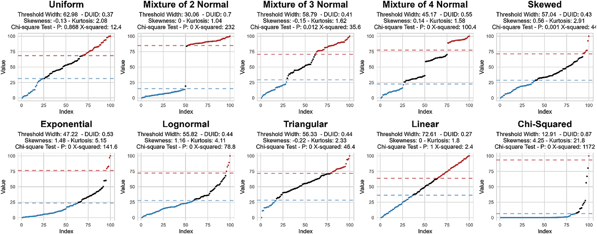
Figure 4: Analysis of ten samples based on density uniformity

The purpose of the chi-squared test is to assess the difference between the sample distribution and the theoretical uniform distribution. Specifically, we compared the observed frequencies of each sample with the expected frequencies to determine whether the samples significantly deviate from a uniform distribution. By calculating the X² statistic, we were able to quantify the degree of this deviation and subsequently analyze the relationship between DUID and X2.

This section clearly demonstrates the correlation between the DUID and the results of the chi-squared test. We generated 1000 time series datasets based on the 10 different distribution characteristics illustrated in Fig. 4, and plotted the relationship between DUID and the chi-square statistic (X2) for these time series data, as shown in Fig. 5. Fig. 5a–c displays the relationship between DUID and the results of the chi-square tests under different numbers of intervals. Through analysis, we found that there is a significant positive correlation between the DUID and the chi-squared statistic (X2).

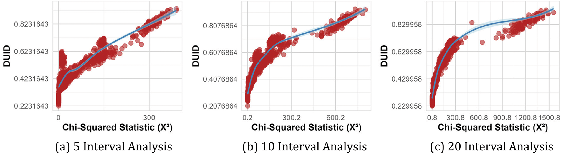
Figure 5: Correlation between DUID and chi-square statistic (X2)

We calculated the correlation coefficients and corresponding p-values between the DUID and the chi-squared statistic (X2) using Kendall’s Tau and Spearman correlation coefficients. The results are presented in Table 2.

From the results above, both Kendall’s Tau and Spearman correlation coefficients indicate a strong positive correlation between the DUID and the chi-squared statistic (X2), with p-values less than 0.001. This suggests that the correlation is highly statistically significant.

In summary, the DUID demonstrates good performance in load time series analysis, effectively identifying and quantifying the characteristics of different load levels, particularly the uniformity of sample distribution density. This provides an important theoretical basis and practical guidance for subsequent load level detection and resource management.

4.4 Evaluation of Algorithm Effectiveness

We conducted a comprehensive performance evaluation of the proposed load level detection algorithm. The evaluation was based on 8 non-parametric scenario samples and 8 parametric synthetic samples, aiming to verify the algorithm’s effectiveness under different data characteristics.

In the non-parametric scenario samples, each sample consists of 72 members, with each member representing a load value. The characteristics of the 8 data sets are illustrated in Fig. 6a, which displays the distribution features and load patterns of the different samples. In the parametric synthetic samples, each sample consists of 300 members, with each member also representing a load value. The characteristics of the 8 data sets are shown in Fig. 6b, further enriching the diversity and complexity of the samples. A detailed description of all 16 samples is provided in Table 3.

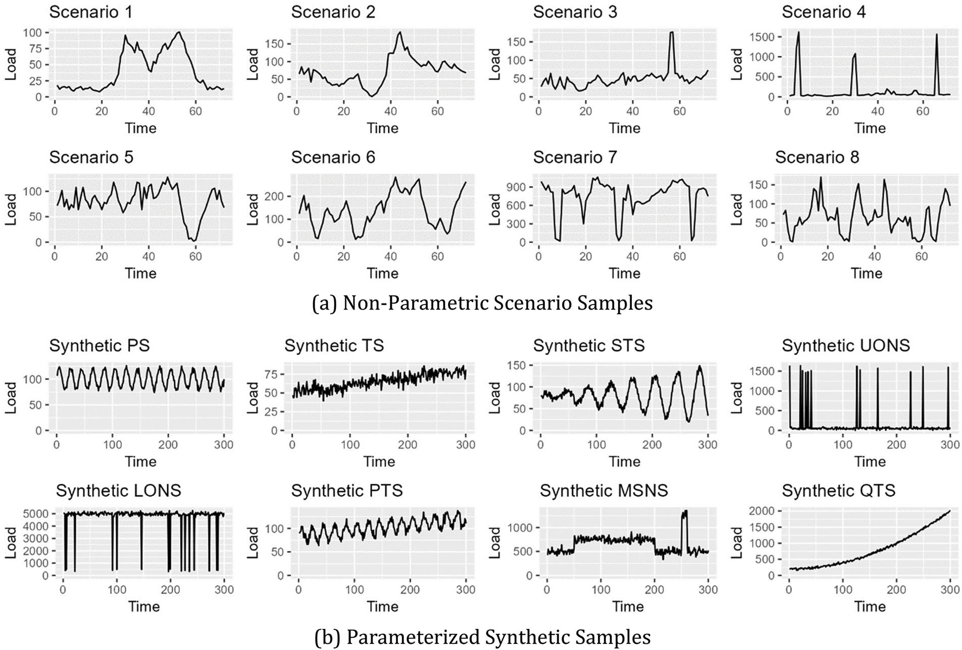
Figure 6: Visualization of 16 load time series samples

We visually presented the algorithm’s results for the 16 samples. Each sample’s visualization consists of two subplots. The first subplot is a line chart, where the red-marked points indicate high-level loads identified by the algorithm, the blue-marked points represent low-level loads, and the remaining points denote regular loads. The second subplot features an improved Pareto chart. In this chart, we replaced the cumulative percentage line traditionally found in Pareto charts with the load percentages of different load types. The labels on the bars indicate the proportion of each load type relative to the total load, while the X-axis text represents the proportion of the corresponding level load time to the total time. To the right of each sample’s visualization analysis conclusion, the normalized load values at different load levels are displayed.

The algorithm’s results for the scenario samples are shown in Fig. 7. During the execution of the algorithm, the parameters were set as follows: TIQR = 1.5, α = 0.5, and CRef = 150.

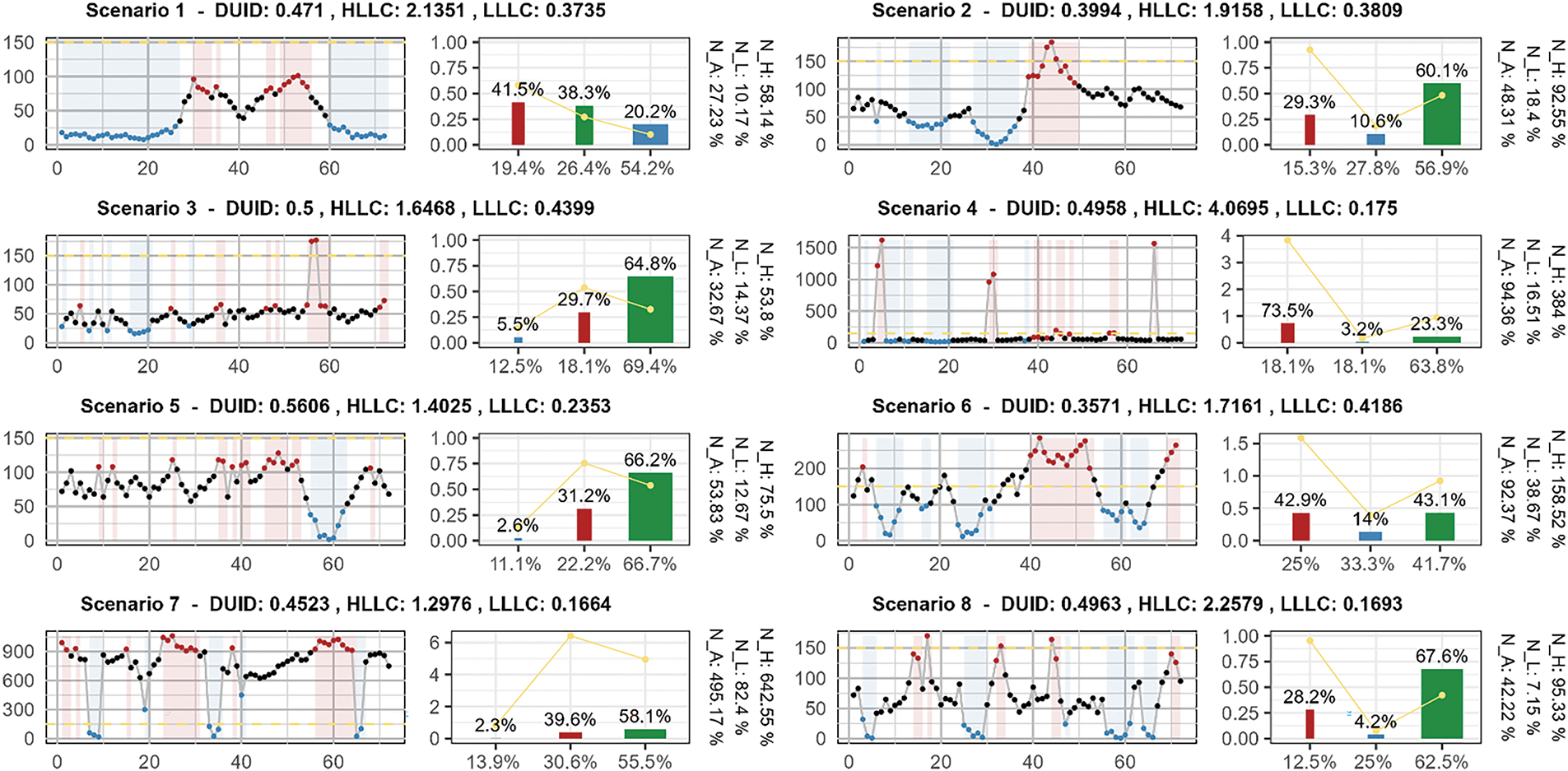
Figure 7: Visualization of algorithm results on non-parametric scenario samples

Taking Scenario 1 as an example, the DUID is 0.471, indicating a moderate degree of uniformity in the sample’s distribution density, with some level of non-uniformity. Therefore, the algorithm does not impose overly strict criteria when identifying high load regions and low load regions. We can observe that during two high load periods, data points are identified as high load regions. The calculation results show that the load amount of the data points identified as high load regions accounts for 41.5%, concentrated within 19.4% of the time. In contrast, the load amount of the data points identified as low load regions only accounts for 20.2%, but is dispersed over 54.2% of the time. The load amount of other data points accounts for a total of 38.3%, distributed over 26.4% of the time. Overall, the results output by the algorithm are reasonable.

Due to space limitations, the algorithm output results for the other 15 samples can be referenced in Fig. 7 and Fig. 8, as well as in Table 4.

Figure 8: Visualization of algorithm results on parameterized synthetic samples

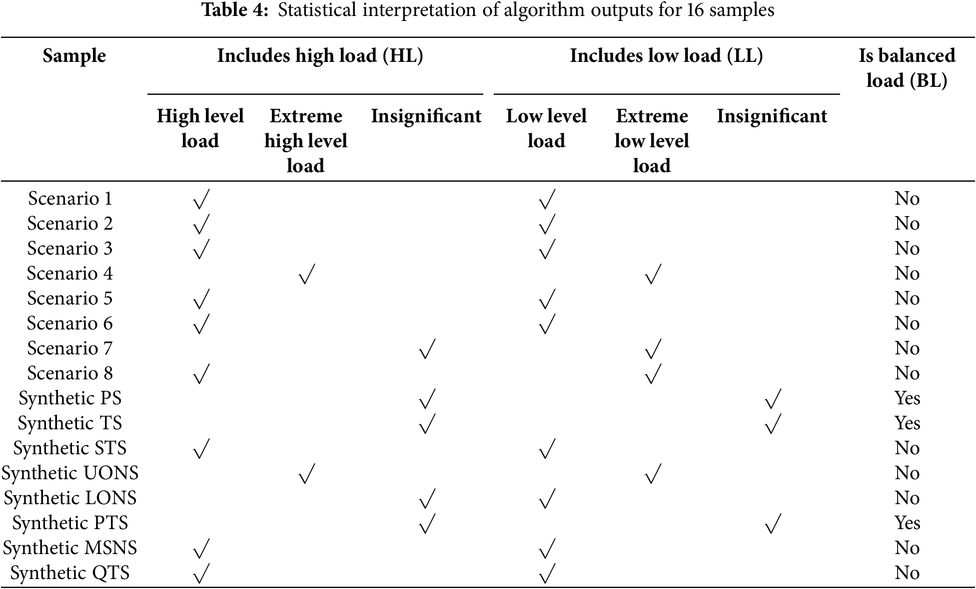
Table 4 summarizes the statistical interpretations of the algorithm’s outputs for the 16 samples. It is noteworthy that the algorithm provides intuitive and easily understandable explanations based on the different characteristics of the samples. For instance, some samples contain Extreme Peak Load, indicating a need to monitor for potential overload situations, while others include Valley Load and Extreme Low Level Load, suggesting that attention should be paid to resource idleness in those samples.

5  Algorithm Validation

5.1 Verification of Algorithm Features

To further validate the effectiveness of the algorithm, we applied the Bootstrap sampling method 1000 times to each of the 16 load time series samples with different characteristics mentioned in Section 4.2. We used the 60%, 75%, 90%, and 95% percentiles of the input samples as references for the high load level thresholds, while the 5%, 10%, 25%, and 40% percentiles of the input samples were used as references for the low load level thresholds for the analysis.

In each bootstrap sample, we identify the regions of different load levels based on the established load level thresholds. Subsequently, we calculate the HLLC and LLLC based on the identification results, using the 2.5% and 97.5% percentiles as the boundaries for the confidence intervals. Finally, we compare the calculated confidence intervals with the values obtained from the TRLLD algorithm proposed in this paper to determine whether they fall within the corresponding confidence intervals.

Through this method, we are able to systematically assess the conclusion preferences of the TRLLD algorithm, thereby validating the effectiveness of automated threshold detection on samples with different characteristics. All statistical results are retained to two decimal places to ensure the precision and readability of the results.

For ease of comparison, the DUID in Tables 4 and 5 is calculated using the input samples after outlier removal, while DUID′ is calculated using the original input samples.

According to Tables 5 and 6, it is evident that as the DUID increases, the HLLC obtained by the TRLLD algorithm tends to fall within the confidence intervals defined by more extreme percentiles for high load level thresholds, such as the 90% and 95% percentiles. Conversely, the LLLC tends to fall within the confidence intervals defined by more extreme percentiles for low load level thresholds, such as the 10% and 5% percentiles. When the DUID is lower, the opposite trend is observed.

This indicates that the proposed algorithm can flexibly adjust the recognition thresholds based on load variations, demonstrating that the algorithm can automatically adjust the high and low load thresholds according to the uniformity of the load distribution (as measured by the DUID index) and accurately identify significant load changes. This validates the effectiveness and adaptability of the TRLLD algorithm in processing load time series.

5.2 Robustness Verification

To validate the robustness of the algorithm, we introduced five different levels of additive noise: 3%, 5%, 10%, and 25% for each data set, and then recalculated the HLLC and LLLC. Subsequently, we assessed the differences between these values and the HLLC and LLLC obtained before the introduction of noise.

The intensity of the introduced noise was determined by calculating the Median Absolute Deviation (MAD) of the original data and adjusting it based on the specified noise percentage. The generated noise followed a normal distribution with a mean of 0 and a standard deviation equal to MAD multiplied by the noise percentage. To ensure the validity of the data, any generated negative values were set to zero. The noise introduced in this manner can moderately simulate uncertainties in real-world scenarios, helping to validate the algorithm’s performance under different noise intensities. The HLLC and LLLC calculated after introducing varying levels of noise are shown in Fig. 9a and b, respectively.

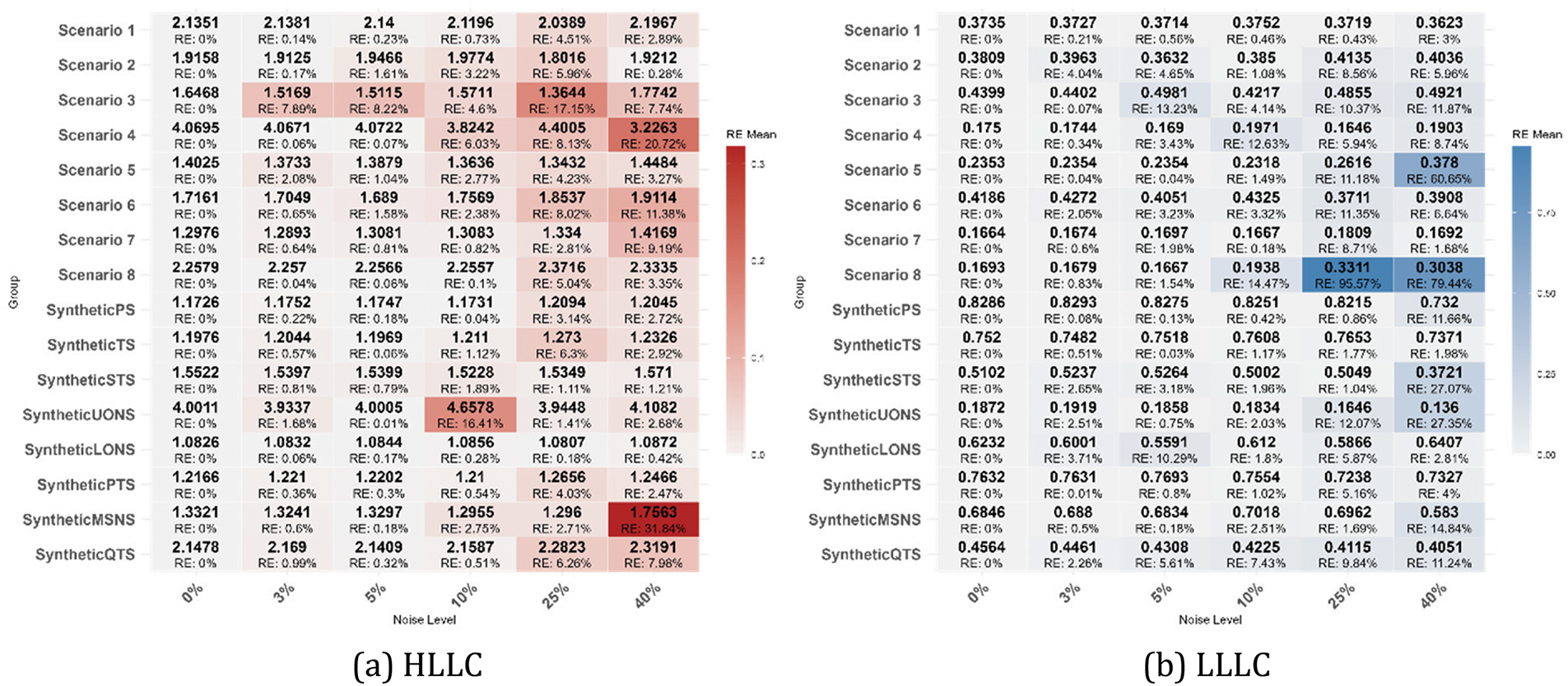
Figure 9: Heatmap of HLLC and LLLC relative errors with varying noise levels

According to Fig. 9, we can observe that when the introduced noise intensity is at 10% or below, the relative errors remain at a low level. It is only when the noise intensity reaches 25% or 40% that some samples exhibit relative errors exceeding 5%. The average relative errors for the eight scenario samples and the eight synthetic samples are presented in Table 7.

According to the results in Table 7, under the introduction of 3%, 5%, and 10% noise, the relative errors for both HLLC and LLLC are all below 5%, with the highest being only 4.72%. The statistical interpretations of the algorithmic analysis conclusions for each sample remain unchanged.

In summary, this indicates that the TRLLD algorithm demonstrates excellent performance when faced with low to moderate levels of additive noise, maintaining high robustness and consistency. This suggests that the algorithm can effectively handle data uncertainty in practical applications, further enhancing its reliability in real-world scenarios.

6  Discussion

The TRLLD algorithm described in this paper is a load level detection algorithm based on threshold recognition using the DUID, representing a relatively foundational research effort in this field. The statistical interpretations provided in this study also lay the groundwork for further applications of this algorithm in engineering contexts.

Currently, most research focuses more on peak and trough detection (extreme point detection) and load forecasting within load time series. Conducting systematic and foundational research on load time series can effectively promote the overall development of this field.

This study demonstrates certain advantages over existing research. Compared to the simple peak detection algorithm proposed by Palshikar [17], the TRLLD algorithm presented in this paper effectively identifies features of load time series by automatically recognizing peaks and troughs and utilizing the DUID, thereby enhancing accuracy and robustness in complex load time series. Gokcesu et al. proposed a non-parametric method for envelope extraction and peak detection in time series by minimizing cumulative L1 drift, achieving a near-linear time complexity [40]. The TRLLD algorithm described in this paper has a time complexity of O(nlog⁡n), primarily due to the sorting operations involved in feature extraction. The TRLLD algorithm is also a non-parametric method, offering multiple perspectives, which enhances its applicability across a wider range of scenarios. The multi-scale method by Messer et al. [41], which combines statistical testing with peak position estimation, performs excellently in the study of neuronal activity; however, the TRLLD algorithm provides a more comprehensive description of load time series features by introducing HLLC and LLLC to quantify load characteristics. The online two-stage peak detection algorithm (TSPD) by Gupta et al. [21] improves adaptability through parameter adjustment, while the TRLLD algorithm also offers two adjustable parameters to optimize sensitivity to outliers and threshold settings, thereby enhancing adaptability and performance across various application domains.

The findings of this study can also be utilized to improve existing research. In the field of load peak and trough detection, this research can enhance the accuracy and sensitivity of peak and trough detection by introducing the DUID, or selectively identifying peak and trough data points with demand characteristics.

In the field of load forecasting, this study can be utilized to enhance the training process of existing forecasting models. The TRLLD algorithm effectively identifies and classifies different load levels, generating high-quality training data that can serve as input for various predictive models, such as LSTM [42] and Transformer [43], thereby enhancing their adaptability to complex dynamic load variations. For LSTM, the load level annotations and time series features from TRLLD help capture temporal dependencies, improving the accuracy of short-term load forecasts. Additionally, HLLC and LLLC can be calculated at a finer granularity to further optimize model performance. For Transformer, the load feature information from TRLLD enhances the effectiveness of the self-attention mechanism, improving the understanding of long-term dependencies and complex load patterns, thereby increasing prediction accuracy. By integrating the outputs of TRLLD, models such as LSTM and Transformer can more accurately forecast future loads when faced with complex load variations, thereby expanding the application potential of deep learning models.

Although the TRLLD algorithm proposed in this paper demonstrates good performance and robustness in load time series analysis, there remain many unexplored areas in the overall interpretability of load time series characteristics. The dynamic evolution of load time series is crucial for resource management and decision support. Future research could focus on the relationship between long-term trends and short-term fluctuations in load behavior, integrating temporal analysis and forecasting models to delve into the driving factors and influencing mechanisms behind load variations. Additionally, further summarizing quantitative metrics for load time series is a mainstream direction.

7  Conclusion

This study proposes the TRLLD algorithm that effectively identifies and classifies high and low load regions within load time series data. The algorithm described in this paper demonstrates enhanced adaptability and accuracy in handling complex load time series by introducing a DUID, thereby providing more dimensional information for further research on load time series.

The experimental results indicate that the proposed DUID effectively reflects the distribution density uniformity of load time series. The TRLLD algorithm can effectively identify regions with different load levels in 16 load time series samples of various distribution types and calculate the load concentration index. Validation results demonstrate that the algorithm can automatically adjust the thresholds for high and low loads based on the uniformity of load distribution (as measured by the DUID index), exhibiting good robustness. Even with the introduction of noise levels of 3%, 5%, and 10%, the relative errors for HLLC and LLLC did not exceed 5%, with a maximum error of only 4.72%.

However, this paper has certain limitations. Specifically, the performance of the TRLLD algorithm on larger datasets has not been thoroughly investigated, and there is a lack of targeted exploration in specific industry segments. Future research should focus on assessing the adaptability and performance of TRLLD in large-scale load time series datasets or datasets from specific industry segments. Nevertheless, due to the temporal correlation commonly found in load time series data, larger datasets can achieve results comparable to those presented in this study by reducing the time granularity, thereby ensuring the algorithm remains feasible in practical applications.

Further discussions require the introduction of more diverse and complex samples, as well as the exploration of new quantitative metrics. A current challenge is the insufficient availability of large-scale load time series samples. Future goals include incorporating additional data samples to create a more rigorous dataset that captures both long-term trends and short-term fluctuations in load behavior, such as the relationship between long-term trends and short-term volatility, as well as the load volatility index. Applying the TRLLD algorithm to time series forecasting models such as LSTM and Transformer is also one of the primary research directions for the future. Additionally, further validation of the applicability of TRLLD and related metrics like DUID in practical scenarios across different fields is also a key objective for future research. Through these efforts, we aim to advance the theoretical and practical development of load time series analysis and promote research progress in related fields.

Acknowledgement: I would like to express my sincere gratitude to Professor Kharin Aleksey Y. for the insightful statistical testing concepts shared during his lecture. His ideas greatly inspired me and helped me to better apply statistical methods in this research.

Funding Statement: The authors received no specific funding for this study.

Author Contributions: The authors confirm contribution to the paper as follows: Conceptualization, Qingqing Song; methodology, Qingqing Song; software, Qingqing Song and Shaoliang Xia; validation, Qingqing Song, Shaoliang Xia, and Zhen Wu; formal analysis, Qingqing Song and Shaoliang Xia; investigation, Qingqing Song; resources, Qingqing Song; data curation, Qingqing Song; writing, original draft preparation, Qingqing Song; writing, review and editing, Qingqing Song, Shaoliang Xia, and Zhen Wu; visualization, Zhen Wu; project administration, Qingqing Song. All authors reviewed the results and approved the final version of the manuscript.

Availability of Data and Materials: Not applicable.

Ethics Approval: Not applicable.

Conflicts of Interest: The authors declare no conflicts of interest to report regarding the present study.

References

1. Samet H, Khorshidsavar M. Analytic time series load flow. Renew Sustain Energy Rev. 2018;82(2):3886–99. doi:10.1016/j.rser.2017.10.084. [Google Scholar] [CrossRef]

2. Choi K, Yi J, Park C, Yoon S. Deep learning for anomaly detection in time-series data: review, analysis, and guidelines. IEEE Access. 2021;9:120043–65. doi:10.1109/ACCESS.2021.3107975. [Google Scholar] [CrossRef]

3. Pereira LES, da Costa VM. Interval analysis applied to the maximum loading point of electric power systems considering load data uncertainties. Int J Electr Power Energy Syst. 2014;54(6):334–40. doi:10.1016/j.ijepes.2013.07.026. [Google Scholar] [CrossRef]

4. Hu S, Gao Z, Wu J, Ge Y, Li J, Zhang L, et al. Time-interval-varying optimal power dispatch strategy based on net load time-series characteristics. Energies. 2022;15(4):1582. doi:10.3390/en15041582. [Google Scholar] [CrossRef]

5. Song Q, Wu Z, Xia S. Node load rate calculation method based on database query statistics in load balancing strategy. In: 2024 Asia-Pacific Conference on Image Processing, Electronics and Computers (IPEC); 2024 Apr 12–14; Dalian, China: IEEE; 2024. p. 408–12. doi:10.1109/IPEC61310.2024.00077. [Google Scholar] [CrossRef]

6. Liu G, Liu J, Bai Y, Wang C, Wang H, Zhao H, et al. EWELD: a large-scale industrial and commercial load dataset in extreme weather events. Sci Data. 2023;10(1):615. doi:10.1038/s41597-023-02503-6. [Google Scholar] [PubMed] [CrossRef]

7. Zhou K, Hu D, Hu R, Zhou J. High-resolution electric power load data of an industrial park with multiple types of buildings in China. Sci Data. 2023;10(1):870. doi:10.1038/s41597-023-02786-9. [Google Scholar] [PubMed] [CrossRef]

8. Bhalaji N. Cloud load estimation with deep logarithmic network for workload and time series optimization. J Soft Comput Paradigm. 2021;3(3):234–48. doi:10.36548/jscp. [Google Scholar] [CrossRef]

9. Yadav MP, Pal N, Yadav DK. Workload prediction over cloud server using time series data. In: 2021 11th International Conference on Cloud Computing, Data Science & Engineering (Confluence); 2021 Jan 28–29; Noida, India: IEEE; 2021. p. 267–72. doi:10.1109/confluence51648.2021.9377032. [Google Scholar] [CrossRef]

10. Khan A, Yan X, Tao S, Anerousis N. Workload characterization and prediction in the cloud: a multiple time series approach. In: 2012 IEEE Network Operations and Management Symposium; 2012 Apr 16–20; Maui, HI, USA: IEEE; 2012. p. 1287–94. doi:10.1109/NOMS.2012.6212065. [Google Scholar] [CrossRef]

11. Higginson AS, Dediu M, Arsene O, Paton NW, Embury SM. Database workload capacity planning using time series analysis and machine learning. In: Proceedings of the 2020 ACM SIGMOD International Conference on Management of Data; Portland OR USA: ACM; 2020. p. 769–83. doi:10.1145/3318464. [Google Scholar] [CrossRef]

12. McDonald R. Time series forecasting of database workloads in hybrid cloud [dissertation]. Dublin, Ireland: National College of Ireland; 2021. [Google Scholar]

13. Hagan MT, Behr SM. The time series approach to short term load forecasting. IEEE Trans Power Syst. 1987;2(3):785–91. doi:10.1109/TPWRS.1987.4335210. [Google Scholar] [CrossRef]

14. Motlagh O, Berry A, O’Neil L. Clustering of residential electricity customers using load time series. Appl Energy. 2019;237(1):11–24. doi:10.1016/j.apenergy.2018.12.063. [Google Scholar] [CrossRef]

15. Shilpa GN, Sheshadri GS. Electrical load forecasting using time series analysis. In: 2020 IEEE Bangalore Humanitarian Technology Conference (B-HTC); 2020 Oct 8–10; Vijiyapur, India: IEEE; 2020. p. 1–6. doi:10.1109/b-htc50970.2020.9297986. [Google Scholar] [CrossRef]

16. Loganathan U, Nagarajan G, Gopinath S, Chandrasekar V. Deep learning based photovoltaic generation on time series load forecasting. Bulletin EEI. 2024;13(5):3746–56. doi:10.11591/eei.v13i5.7836. [Google Scholar] [CrossRef]

17. Palshikar G. Simple algorithms for peak detection in time-series. In: Proceedings of the 1st International Conference on Advanced Data Analysis, Business Analytics and Intelligence; 2009; Pune, India. Vol. 122, p. 1–13. [Google Scholar]

18. Schneider R. Survey of peaks/valleys identification in time series [master’s thesis]. Zurich, Switzerland: University of Zurich; 2011. [Google Scholar]

19. Li L, Cao B, Liu Y. A study on CEP-based system status monitoring in cloud computing systems. In: 2013 6th International Conference on Information Management, Innovation Management and Industrial Engineering; 2013 Nov 23–24; Xi’an, China: IEEE; 2013. p. 300–3. doi:10.1109/ICIII.2013.6702934. [Google Scholar] [CrossRef]

20. Cao Z, Lin J, Wan C, Song Y, Zhang Y, Wang X. Optimal cloud computing resource allocation for demand side management in smart grid. IEEE Trans Smart Grid. 2017;8(4):1943–55. doi:10.1109/TSG.2015.2512712. [Google Scholar] [CrossRef]

21. Gupta A, Onumanyi AJ, Ahlawat S, Prasad Y, Singh V. TSPD: a robust online time series two-stage peak detection algorithm. In: 2023 IEEE International Conference on Service-Oriented System Engineering (SOSE); 2023 Jul 17–20; Athens, Greece: IEEE; 2023. p. 91–7. doi:10.1109/SOSE58276.2023.00017. [Google Scholar] [CrossRef]

22. Tsekouras GJ, Salis AD, Tsaroucha MA, Karanasiou IS. Load time-series classification based on pattern recognition methods. Patt Recognit Techni, Techno Appl. 2008;10:361–432. doi:10.5772/6250. [Google Scholar] [CrossRef]

23. Manojlović I, Švenda G, Erdeljan A, Gavrić M. Time series grouping algorithm for load pattern recognition. Comput Ind. 2019;111(1):140–7. doi:10.1016/j.compind.2019.07.009. [Google Scholar] [CrossRef]

24. Qi Y, Luo B, Wang X, Wu L. Load pattern recognition method based on fuzzy clustering and decision tree. In: 2017 IEEE Conference on Energy Internet and Energy System Integration (EI2); 2017 Nov 26–28; Beijing, China: IEEE; 2017. p. 1–5. doi:10.1109/EI2.2017.8245714. [Google Scholar] [CrossRef]

25. Tambunan HB, Barus DH, Hartono J, Alam AS, Nugraha DA, Usman HHH. Electrical peak load clustering analysis using K-means algorithm and silhouette coefficient. In: 2020 International Conference on Technology and Policy in Energy and Electric Power (ICT-PEP); 2020 Sep 23–24; Bandung, Indonesia: IEEE; 2020. p. 258–62. doi:10.1109/ict-pep50916.2020.9249773. [Google Scholar] [CrossRef]

26. Rajabi A, Eskandari M, Ghadi MJ, Li L, Zhang J, Siano P. A comparative study of clustering techniques for electrical load pattern segmentation. Renew Sustain Energy Rev. 2020;120:109628. doi:10.1016/j.rser.2019.109628. [Google Scholar] [CrossRef]

27. Song Q, Xia S. Research on the effectiveness of different outlier detection methods in common data distribution types. J Comput Technol Appl Mathem. 2024;1(1):13–25. doi:10.5281/zenodo.10888672. [Google Scholar] [CrossRef]

28. Shiffler RE. Maximum Z scores and outliers. Am Stat. 1988;42(1):79–80. doi:10.1080/00031305.1988.10475530. [Google Scholar] [CrossRef]

29. Larson MG. Descriptive statistics and graphical displays. Circulation. 2006;114(1):76–81. doi:10.1161/CIRCULATIONAHA.105.584474. [Google Scholar] [PubMed] [CrossRef]

30. Khan K, Rehman SU, Aziz K, Fong S, Sarasvady S. DBSCAN: past, present and future. In: The Fifth International Conference on the Applications of Digital Information and Web Technologies (ICADIWT 2014); 2014 Feb 17–19; Bangalore, India: IEEE; 2014. p. 232–8. doi:10.1109/ICADIWT.2014.6814687. [Google Scholar] [CrossRef]

31. Al Farizi WS, Hidayah I, Rizal MN. Isolation forest based anomaly detection: a systematic literature review. In: 2021 8th International Conference on Information Technology, Computer and Electrical Engineering (ICITACEE); 2021 Sep 23–24; Semarang, Indonesia: IEEE; 2021. p. 118–22. doi:10.1109/icitacee53184.2021.9617498. [Google Scholar] [CrossRef]

32. Mensi A, Cicalese F, Bicego M. Using random forest distances for outlier detection. In: International Conference on Image Analysis and Processing. Lecce, Italy: Springer; 2022. p. 75–86. [Google Scholar]

33. Almardeny Y, Boujnah N, Cleary F. A novel outlier detection method for multivariate data. IEEE Trans Knowl Data Eng. 2022;34(9):4052–62. doi:10.1109/TKDE.2020.3036524. [Google Scholar] [CrossRef]

34. Boukerche A, Zheng L, Alfandi O. Outlier detection: methods, models, and classification. ACM Comput Surv. 2020;53(3):1–37. doi:10.1145/3421763. [Google Scholar] [CrossRef]

35. Blázquez-García A, Conde A, Mori U, Lozano JA. A review on outlier/anomaly detection in time series data. ACM Comput Surv. 2021;54(3):1–33. doi:10.1145/3444690. [Google Scholar] [CrossRef]

36. Zamanzadeh Darban Z, Webb GI, Pan S, Aggarwal C, Salehi M. Deep learning for time series anomaly detection: a survey. ACM Comput Surv. 2025;57(1):1–42. doi:10.1145/3691338. [Google Scholar] [CrossRef]

37. Luo J, Hong T, Yue M. Real-time anomaly detection for very short-term load forecasting. J Mod Power Syst Clean Energy. 2018;6(2):235–43. doi:10.1007/s40565-017-0351-7. [Google Scholar] [CrossRef]

38. Yue M, Hong T, Wang J. Descriptive analytics-based anomaly detection for cybersecure load forecasting. IEEE Trans Smart Grid. 2019;10(6):5964–74. doi:10.1109/TSG.2019.2894334. [Google Scholar] [CrossRef]

39. Cook AA, Mısırlı G, Fan Z. Anomaly detection for IoT time-series data: a survey. IEEE Internet Things J. 2020;7(7):6481–94. doi:10.1109/JIOT.2019.2958185. [Google Scholar] [CrossRef]

40. Gokcesu K, Gokcesu H. Nonparametric extrema analysis in time series for envelope extraction, peak detection and clustering. arXiv:2109.02082. 2021. [Google Scholar]

41. Messer M, Backhaus H, Fu T, Stroh A, Schneider G. A multi-scale approach for testing and detecting peaks in time series. Statistics. 2020;54(5):1058–80. doi:10.1080/02331888.2020.1823980. [Google Scholar] [CrossRef]

42. Yu Y, Si X, Hu C, Zhang J. A review of recurrent neural networks: LSTM cells and network architectures. Neural Comput. 2019;31(7):1235–70. doi:10.1162/neco_a_01199. [Google Scholar] [PubMed] [CrossRef]

43. Wen Q, Zhou T, Zhang C, Chen W, Ma Z, Yan J, et al. Transformers in time series. In: Proceedings of the Thirty-Second International Joint Conference on Artificial Intelligence; 2023 Aug 19–25; Macau, China: International Joint Conferences on Artificial Intelligence Organization. p. 6778–86. doi:10.24963/ijcai.2023/759. [Google Scholar] [CrossRef]