A Feature Selection Method for Software Defect Prediction Based on Improved Beluga Whale Optimization Algorithm

1  Introduction

Software quality assurance has become a critical challenge in software engineering as the size and complexity of software systems continue to grow. Software defects can not only compromise reliability but also lead to high maintenance costs or even severe system failures. Therefore, SDP has received widespread attention as an effective means of prevention and detection. By analyzing historical code and project data to build a SDP model, potential defect-prone modules can be identified early in the software development process, thereby reducing development risks and improving development efficiency [1]. Previous experiments [2] have predicted the defect tendency of software modules by analyzing various metrics in software source code. These metrics reflect the complexity of the code and related information in the development process, but too many metrics may lead to poor quality of the prediction model. This is because there will be redundant metrics that are irrelevant to defect prediction. Using feature selection can avoid this problem. Feature selection is crucial in SDP. It aims to eliminate irrelevant or redundant features, thereby enhancing model performance, improving training efficiency, and avoiding overfitting [3,4]. In SDP, we may use multiple features such as Coupling Between Objects (CBO), Depth of Inheritance Tree (DIT), Lack of Cohesion in Methods (LCOM), Number of Children (NOC), Response For a Class (RFC), and Weighted Methods per Class (WMC). These features reflect different complexities and design characteristics of classes, but some of them may be redundant or irrelevant. For example, CBO and RFC are often highly correlated because class coupling and response set size are closely related. In contrast, DIT may show a weaker correlation with defect occurrence, making it an irrelevant feature. Feature selection helps boost the prediction accuracy of SDP and speeds up training by eliminating unnecessary or irrelevant features. Therefore, feature selection helps the model focus on truly useful features, enhancing its generalization ability.

Goyal et al. [5] proposed to use lion optimization algorithm for feature selection to enhance the performance of SDP. Malhotra et al. [6] introduced a SDP model that uses a two-phase grey wolf optimization for feature selection, and Chantar et al. [7] proposed using an enhanced binary grey wolf optimizer for text classification. The performance of the population-based metaheuristic algorithm is impacted by initialization and parameter control. In particular, if the population position is not initialized with sufficient randomness and the search space may not be fully explored, which means not all features will be traversed and redundant or irrelevant features will not be effectively removed. Goyal [8] proposed a genetic evolution algorithm for feature selection. Genetic algorithms involve several parameters, including population size, crossover rate, and mutation rate, etc. The choice of these parameters significantly affects the final performance of the algorithm. If these parameters are set unreasonably, the algorithm may converge too slow, thus affecting the final performance of defect prediction. To solve these problems, this study introduces a novel feature selection method CTMBWO based on BWO. As far as we know, BWO has not been used for feature selection in the SDP field. This method generates the initial individual population through Cubic chaotic mapping, which is more random and uniform and can effectively avoid falling into the local optimal solution. And an update mechanism based on the combination of Cauchy mutation and reverse learning is used to effectively boost the diversity and the speed of global convergence of the population. When the current population is not optimal, the triangle wandering strategy is used to update the selected population. At the same time, the algorithm uses a small number of parameters.

The contributions of this paper are as follows:

(1)   In the initialization stage of CTMBWO, the Cubic chaotic map is introduced to generate a more evenly distributed initial population and strengthen the algorithm’s global search ability.

(2)   In the exploration phase of CTMBWO, the triangle walk strategy is used to further expand the search range of the algorithm and improve the search accuracy.

(3)   During the whale fall phase of CTMBWO, an update mechanism based on the combination of Cauchy mutation and reverse learning is used to effectively enhance the distribution and the speed of global convergence of the population. In addition, a sparrow alert mechanism is also integrated to further ensure that the beluga can avoid getting stuck in the local optimal solution.

2  Related Work

Feature selection is crucial in SDP that aims to select the feature subset that has the greatest impact on the prediction results from a lot of features. The dataset may contain a large number of irrelevant and redundant features in SDP, and the excessive number of features may increase the time cost of training the classifier and may reduce the performance of the classifier. When dealing with high-dimensional features, feature selection methods are currently widely used. Feature selection methods are divided into filtering method, wrapping method, and ensemble learning method.

(1)   Filtering method

The filtering method is an unsupervised feature selection method that scores features by evaluating the correlation or divergence of each feature with the target variable individually, without relying on a specific model. This method does not require model training, so it is computationally efficient and suitable for processing large-scale data sets. Based on the scoring results, the filtering method selects features based on a set threshold or the top N highest-scoring features. Some commonly used filtering methods are Chi-Square (CS), Information Gain (IG), Relief method, etc.

(2)   Wrappering method

The wrappering method closely combines feature selection with the model training process and systematically assessing the performance of various feature subsets to identify the most effective ones. The core idea of the wrappering method is to use a specific machine learning algorithmto train the model and evaluate the pros and cons of each feature subset based on the model’s predictive performance. This method can obtain a better feature set, especially when the feature dimension is high. Commonly used methods include forward selection and exhaustive search.

(3)   Ensemble learning method

The ensemble learning method is a combination of filtering and wrapping methods. Features are selected by comprehensively selecting the results of multiple filtering or wrapping methods, or the output of the filtering method is used as the input of the wrapping method to screen features. The ensemble method combines the advantages of filtering and wrapping methods, and often produces better prediction performance than models based on single filtering or wrapping methods.

Population-based metaheuristic algorithms are often used for feature selection, especially in high-dimensional data or complex problems. They can explore the feature space by simulating the natural evolution process and select the most advantageous feature subset.

Das et al. [9] introduced a cutting-edge feature selection method known as the Golden Jackal Optimization (GJO) algorithm, a metaheuristic inspired by the hunting strategies of the golden jackal. The method can be further applied to multi-objective optimization problems by using feature selection. The researchers integrated this algorithm with four classification models to extract significant feature subsets from SDP datasets.

Arasteh et al. [10] proposed an innovative feature selection method by changing the Binary Chaos-based Olympiad Optimization Algorithm. Using this method to get the features that have the greatest impact on the prediction results. Integrating the method with classification models can greatly improve the precision and accuracy of software module classification.

Kukkar et al. [11] proposed a feature extraction technique by improving the ant colony optimization (ACO) to find out more relevant features for SDP. At the same time, the algorithm was integrated with machine learning to boost prediction performance. The results demonstrated a significant improvement in accuracy compared to the baseline methods.

Anbu et al. [12] used the firefly algorithm for feature selection. Fireflies tend to fly towards brighter areas, and their flight direction and distance are influenced by two important factors: brightness and attractiveness. These factors are used to guide the selection of solutions, with fireflies attracted to one another based on brightness differences, ultimately searching for the global optimal solution. Through this process, a representative feature subset is selected.

Wang et al. [13] proposed a binary adaptation of the Gray Wolf Optimizer algorithm aiming at identifying the most impactful features within the dataset to solve the problems of excessive feature volume in the training dataset. Through feature selection, the features that have the greatest impact on the SDP are selected. These features include the number of lines of code and complexity, etc. At the same time, experiments show that accuracy, Recall, and F1 have been significantly improved.

Sekaran et al. [14] proposed a new feature selection method that combines mutation-enhanced Salp Swarm Optimizer (MBSSO) with rough set theory. Rough set theory offers a structured approach to examining the relationships and dependencies among features. It refines the search space by assessing fitness scores and incorporates a mutation enhancement strategy to evade getting stuck at local optima. SDP is performed after feature selection using kernel extreme learning machine.

Alsghaier et al. [15] proposed combining genetic algorithm (GA) with support vector machine (SVM) classifier and particle swarm algorithm (PSO) to obtain better SDP performance. The experimental results show that when applied to limited scale datasets, integrating GA with SVM and PSO can obtain good SDP results and overcome the limitations of previous studies.

Inspired by the above techniques, this paper also uses a population-based metaheuristic algorithm CTMBWO for feature selection. The algorithm uses chaotic mapping [16] to change the initialization method of the population, making the distribution of the population more uniform and random. At the same time, mutation operations are performed during each iteration to find the optimal population and optimal feature subset faster, thereby improving the SDP performance.

3  Proposed Methodology

3.1 Beluga Whale Optimization Algorithm

Beluga whale optimization algorithm (BWO) was proposed by Zhong et al. in 2022 [17], which is a heuristic algorithm based on the beluga’s lifestyle, as shown in Fig. 1. The algorithm simulates the beluga’s swimming behavior (a), praying behavior (b), and death behavior (c) and they are modeled as the exploration, exploitation, and whale-fall phases.

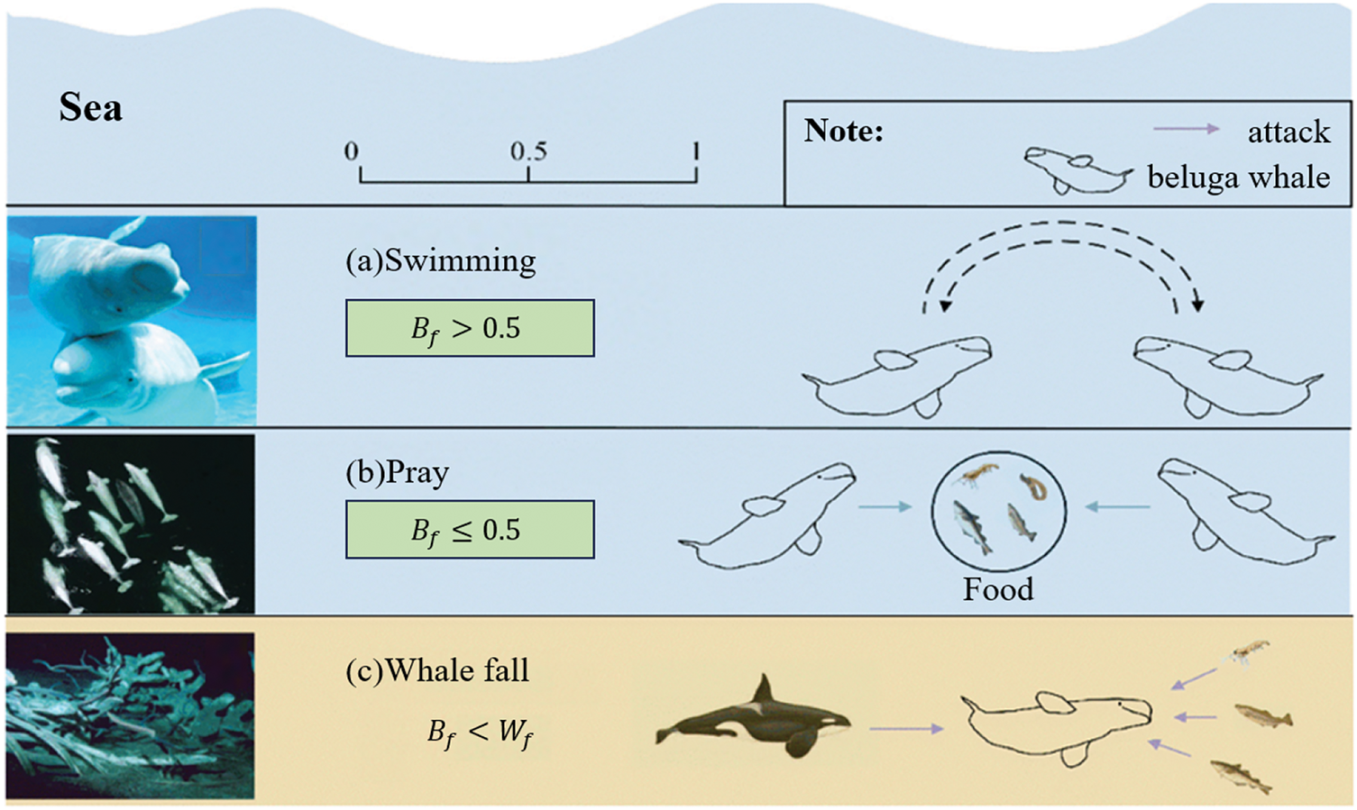
Figure 1: The lifestyle of Beluga, (a) Swimming behavior; (b) Pray behavior; (c) Whale fall behavior

In the feature selection task, BWO searches for the optimal feature subset by representing each feature as a binary vector and simulating the strategy of beluga whales swimming around their prey. The fitness of each beluga whale is calculated and evaluate their performance. The algorithm updates the position of the beluga whale based on the fitness value and gradually selects the most useful features for SDP.

By comparing the balance factor Bf, the BWO decides whether to enter the exploration or exploitation phase. When Bf>0.5 the algorithm is in the exploration phase, and when Bf≤0.5, it shifts to the exploitation phase. The probability Wf and Bf together determine whether the whale fall phase occurs and it happens when Bf<Wf. The mathematical model of Bf and Wf are:

Bf=B0(1−T/2Tmax)(1)

Wf=0.1−0.05T/Tmax(2)

where T is the iteration number currently being executed, Tmax is the maximum iterative number, B0 is a random number between (0, 1).

3.1.1 Initialization Phase

In the initialization stage, BWO randomly generates a population of beluga whales and calculates the fitness value corresponding to each population. It determines whether the current population is optimal by comparing the fitness value. Using the matrix X to represent the obtained population.

3.1.2 Exploration Phase

When Bf>0.5, the algorithm enters the exploration phase. In this phase, the beluga whales swim randomly in all directions to locate the global optimal solution and avoid getting trapped in local optima. The updated position of the beluga whale is expressed as:

{Xi,jT+1=Xi,pjT+(Xr,p1T−Xi,pjT)(1+r1)sin⁡(2πr2)j=evenXi,jT+1=Xi,pjT+(Xr,p1T−Xi,pjT)(1+r1)cos⁡(2πr2)j=odd(3)

where T is the current iteration, Xi,jT+1 is the new position of the ith beluga whale on the jth dimension, pj(j=1,2,⋯,d) is a randomly chosen dimension from the d-dimension, Xi,pjT is the position of the ith beluga whale on pj dimension, Xr,p1T is the current positions of the rth beluga whale (r is the beluga whale chosen at random), r1 and r2 are random number between (0,1), sin⁡(2πr2) and cos⁡(2πr2) denote the fin orientation of the mirrored beluga, with odd and even choices.

3.1.3 Exploitation Phase

The exploitation phase happens when Bf≤0.5. In this stage beluga whale uses the Levy flight strategy [18] to enhance convergence to approach the target solution more accurately by hunting prey.

3.1.4 Whale Fall

The whale fall happens when Bf<Wf. In this stage the beluga whale abandons inferior prey or focuses on catching high-quality prey and further converging to the optimal solution. This stage ensures that the algorithm focuses on optimizing the current best solution, thereby improving the accuracy and reliability of the final result.

3.2 Boosted Beluga Whale Optimization Algorithm CTMBWO

As the feature dimension increases, the feature selection method based on BWO will easily fall into local optimal solutions and uneven population distribution that makes it difficult to choose a feature subset that is both highly accurate in classification and has a limited number of features. In BWO, the distribution of its population is shown in Fig. 2a. Most of the populations are distributed in the lower left corner and the distribution is not uniform. Therefore, when selecting features, processing these densely distributed populations in the lower left corner increases the possibility of obtaining a local optimal solution. The population distribution of CTMBWO is shown in Fig. 2b, which shows that it is evenly distributed. This ensures that all populations will be calculated, and the solution obtained is also the global optimal solution rather than the local optimal solution.

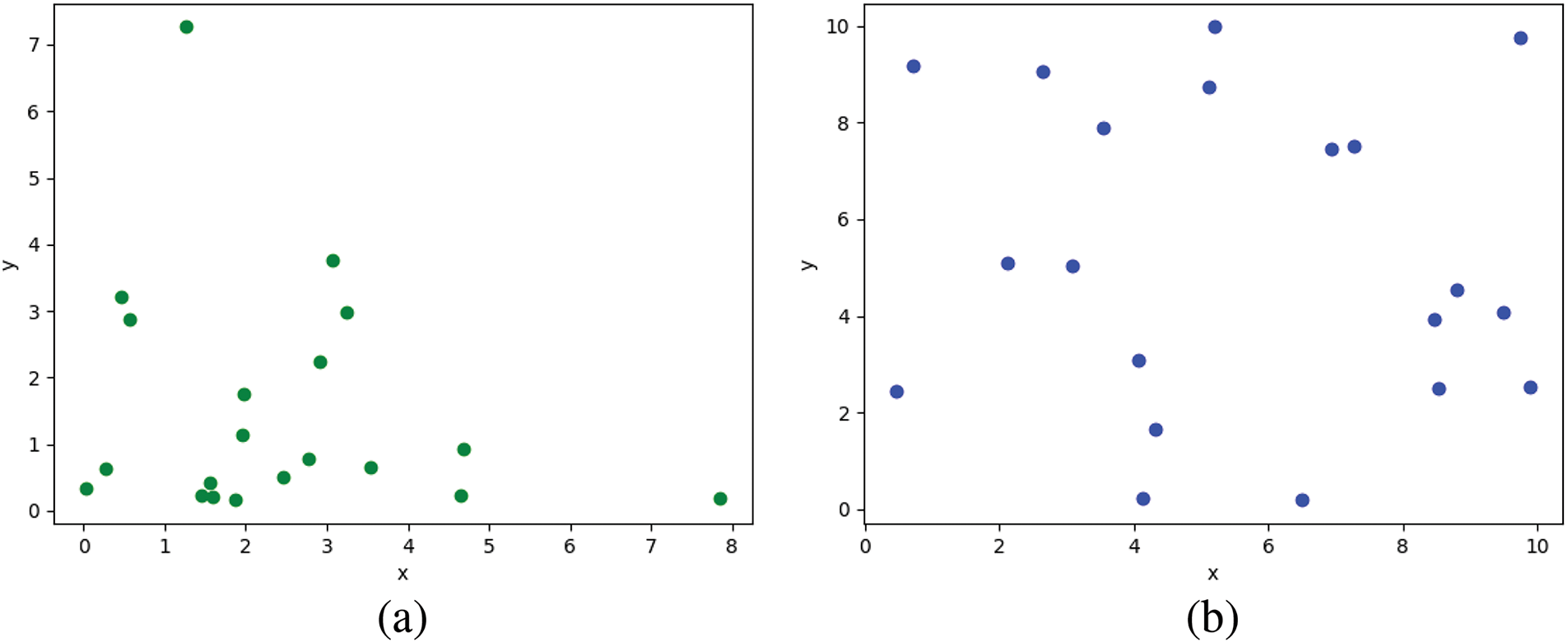
Figure 2: Comparison of population distribution between BWO and CTMBWO, (a) The population distribution of BWO, (b) The population distribution of CTMBWO

3.2.1 Cubic Chaos Mapping

A diverse population will have a significant impact on the predicted results. However, the way BWO generates populations often leads to an uneven distribution, which in turn reduces diversity. To improve the global search capability, it is essential for the beluga whale population to be evenly distributed across the entire search space. Chaotic mapping [16] is known for its randomness, regularity and ergodicity, which can help achieve even distribution and increase population diversity. Therefore, this paper introduces a chaotic iterative mapping based on the Cubic, the formula is as follows:

xn+1=ρxn(1−xn2)(4)

where xn denotes the position of the nth population, ρ denotes the mixing factor and the Cubic mapping has better chaotic traversal when x0 = 0.3, β = 0.259. By using Eq. (4), the new population initialization is obtained as:

X′=(x1,1′x1,2′⋯x1,d′x2,1′x2,2′⋯x2,d′⋮⋮⋱⋮xn,1′xn,2′⋯xn,d′)(5)

and calculate the fitness value:

Ffv=(f(x1,1′,x1,2′,⋯,x1,d′)f(x2,1′,x2,2′,⋯,x2,d′)⋮f(xn,1′,xn,2′,⋯,xn,d′))(6)

where n is the size of the beluga whale population, d is the number of dimensions associated with the design variable.

3.2.2 Triangle Wandering Strategy

(1)   The distance dis between the beluga whale and its conspecifics is expressed as:

dis=XbestT−XiT(7)

(2)   The range of the beluga whale’s walking step length range, is expressed as:

range=α⋅dis1(8)

where α is a normally distributed random number.

(3)   Define the direction β of the beluga whale’s movement and express it as:

β=2πα(9)

where α is a normally distributed random number.

(4)   Calculate the final distance Dist between the wandering position and the same type by using Eqs. (7) and (9):

Dist=dis2+range2−2⋅dis⋅range⋅cos⁡(β)(10)

(5)   The updated position is expressed as:

{Xi,jT+1=Xi,pjT+(Xr,p1T−Xi,pjT)(1+r1)sin⁡(2πr2)+Dist⋅rand(0,1)j=evenXi,jT+1=Xi,pjT+(Xr,p1T−Xi,pjT)(1+r1)cos⁡(2πr2)+Dist⋅rand(0,1)j=odd(11)

where T is the current iteration, Xi,jT+1 is the new position for the ith beluga whale on the jth dimension, pj(j=1,2,⋯,d) is a randomly chosen dimension from d-dimension, Xi,pjT is the position of the ith beluga whale on pj dimension, Xr,p1T is the current positions of the rth beluga whale (r is the beluga whale chosen at random), r1 and r2 are random number between (0, 1), sin⁡(2πr2) and cos⁡(2πr2) denote the fin orientation of the mirrored beluga, with odd and even choices.

3.2.3 Cauchy Mutation Combined with Reverse Learning

During the whale fall phase, Cauchy mutation and reverse learning strategies are used to update the beluga whale’s position to avoid getting stuck into local optima.

In BWO, the target position is updated based on the position change after each iteration and the fitness value is recalculated so the new position replaces the target position. However, the target position remains unaffected which may lead to the algorithm trapped by local optimal solution. Therefore, a strategy of combining Cauchy mutation and reverse learning is proposed to randomly update the target position based on a random probability P to prevent the algorithm from converging to the local optimal solution. The mathematical model of the whale fall stage is:

XiT+1=r5XiT−r6XrT+r7Xstep+XnewT+1(12)

Ps=−exp⁡(1−TTmax)10+ω(13)

XbestT∗=ub+r(lb−XbestT)(14)

{XnewT+1=b3(XnewT−XbestT∗)XnewT+1=Cauchy(0,1)XbestT(15)

where r5, r6, r7, r are random numbers from 0 to 1, Xstep is the movement size during the whale fall stage, Xstep=(ub−lb)exp⁡(−C2T/Tmax) where C2 is the scaling factor for the movement size, C2=2Wf×n, ub and lb are the maximum and minimum limits, ω is the adjustment factor, and the optimal result of the function is obtained when ω is equal to 0.05, XbestT∗ is the reverse solution of the generation T target solution XbestT, XnewT+1 is the generation T+1 target solution, Cauchy(0,1) is the standard Cauchy distribution function, b3 is the pseudo-information exchange coefficient, b3=αe(−βT)/Tmax, α is the random initial value, β is the decay rate, T is the iteration number currently being executed, Tmax is the maximum iterative number.

3.2.4 Sparrow Alert Mechanism

In the whale fall phase, the failed individuals can share useful information with other individuals by simulating the behavior of alert individuals in the sparrow alert mechanism, thereby transmitting environmental risks. This information may include the search space situation around the failed individuals and help other individuals avoid being confined to the same solution or further optimize their own solutions. The formula is:

XiT+1=XiT+α(XnewT+1−XiT)+βR(16)

where XiT+1 is the position of the current individual i in generation T+1, XnewT+1 is the target solution of generation T+1, α is a scaling factor to control the direction of the individual’s movement, β is a scaling factor to control the scope of the randomized search and R is a random vector, which is used to guide the individual to perform the randomized search and increase the stochasticity and diversity of the exploration.

3.2.5 Summary of CTMBWO Algorithm

Fig. 3 is the algorithm flow chart of CTMBWO.

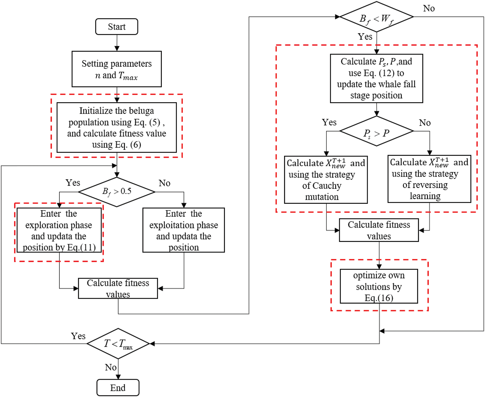
Figure 3: The algorithm flow chart of CTMBWO

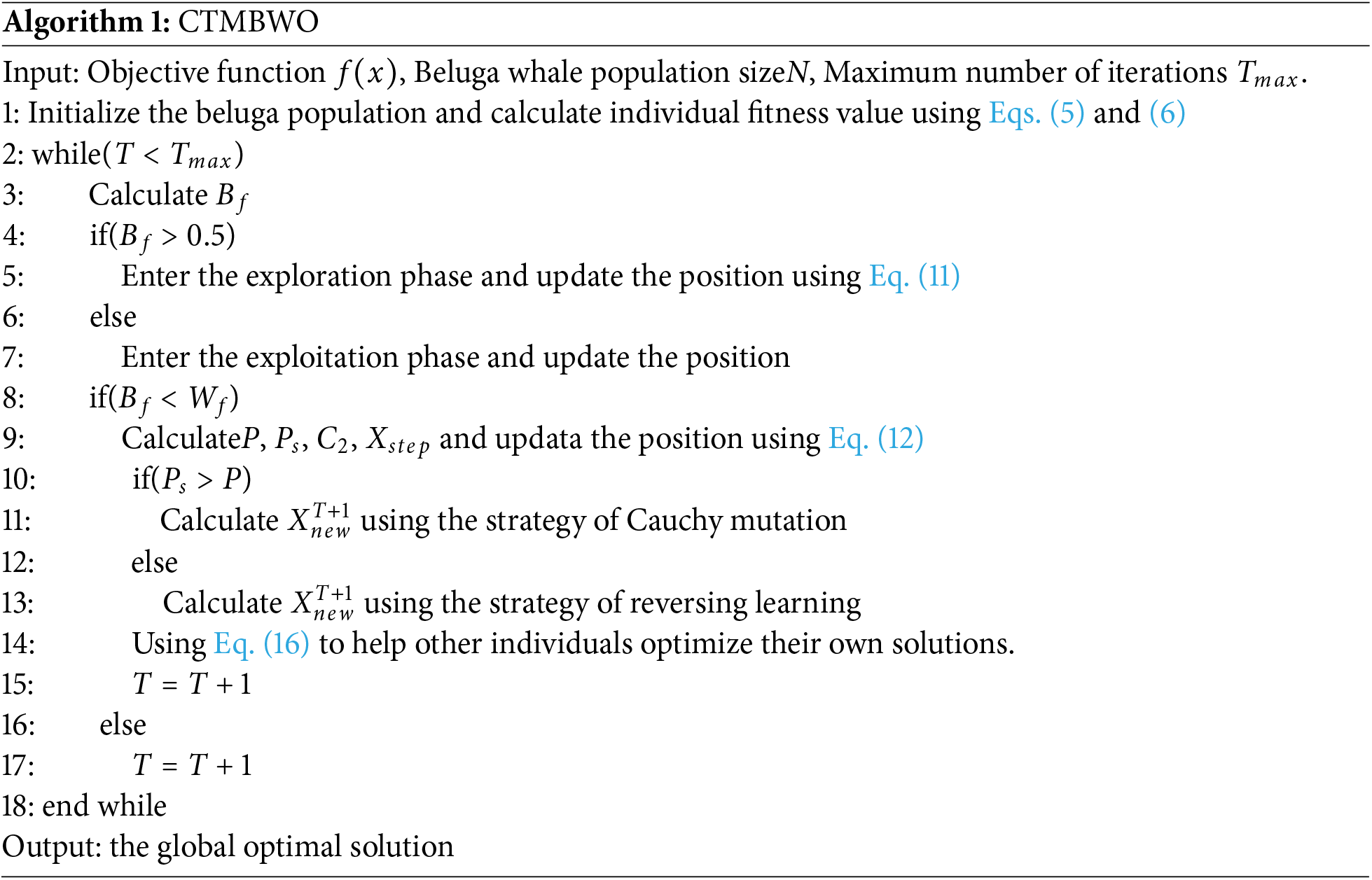
The specific algorithm of CTMBWO is as shown in Algorithm 1.

4  Experimental Design

4.1 Experimental Condition

The experiments in this paper are conducted using Python 3.9 on 64-bit Windows 10 operating system, with Pycharm and an i7-10700F CPU.

4.2 Datasets

The datasets used in this paper are 19 projects from NASA and PROMISE. The datasets details are shown in Table 1.

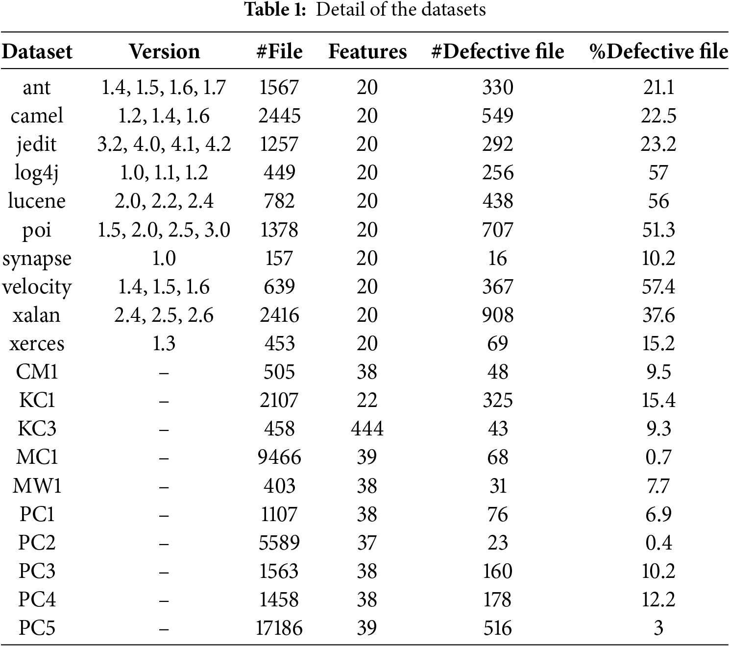
By further observing the specific feature values of each project in Table 1, it can be found that the feature value distribution in the data set has a large range of differences. For example, in project ant-1.5, the value of WMC is 9, the value of DIT is 6, the value of LCOM3 is 0.8125, and the value of AMC is 17.2222. This difference in numerical range will affect the model’s processing of features. To address this problem we use Min-Max normalization [19] that scales the data and ensures that all numbers have the same range, thereby eliminating the numerical differences between different features. The formula is:

X′=X−XminXmax−Xmin(17)

where Xmax and Xmin are the maximum and minimum values of the features. According to the Pareto principle, about 80% of software defects occur in about 20% of software modules [20]. And the sample size for particular categories in the dataset that we use is far less than that in other categories. To effectively address this problem, we adopted the Synthetic Minority Over-sampling Technique (SMOTE) [21], which generates synthetic samples by oversampling the minority class to balance the class distribution.

To assess the stability and generalization capability of the proposed method, we employ 5-fold cross-validation. The dataset is split evenly into 5 subsets, with 4 subsets used for training in each iteration and the remaining one used for testing. This process is repeated 5 times, and the final result is the average of all 5 runs. By doing so, each subset is used as a test set at least once, enhancing the model’s overall reliability and robustness. At the same time, we employ a strategy combining cross-validation and early stopping to further prevent overfitting.

4.3 Baseline Model

The benchmark models used are four well-known models GAPSO [15], Fed-OLF [22], MFWFS [23], and SLSTM [24].

4.4 Evaluate Metrics

We evaluate the prediction model’s performance using widely recognized metrics, accuracy, precision, recall, F1, and the area under the curve (AUC). In addition, we use the Matthews Correlation Coefficient (MCC) that is a more comprehensive performance indicator. The formulas are:

Accuracy=TN+TPTN+TP+FN+FP(18)

Precision=TPTP+FP(19)

Recall=TPTP+FN(20)

F−measure=2×Precision×RecallPrecision+Recall(21)

MCC=TP×TN−FP×FN(TP+FP)(TP+FN)(TN+FP)(TN+FN)(22)

where TP is True Positive that refers to the cases where the sample is positive, and the model also predicts it as positive, TN is True Negative that refers to the cases where the sample is negative, and the model predicts it as negative as well, FN is False Negative that refers to the cases where the actual class is positive, but the model predicts it as negative, FP is False Positive that refers to the cases where the actual class is negative, but the model predicts it as positive. AUC is the area under the receiver operating characteristic curve (ROC). ROC curve is an effective tool for evaluating the performance of binary classification models. By plotting the false positive rate and recall at different classification thresholds, it helps us gain a comprehensive understanding of the model’s performance under various conditions. The AUC measures the discriminatory ability of the classification model, with values closer to 1 indicating better classification performance.

5  Result

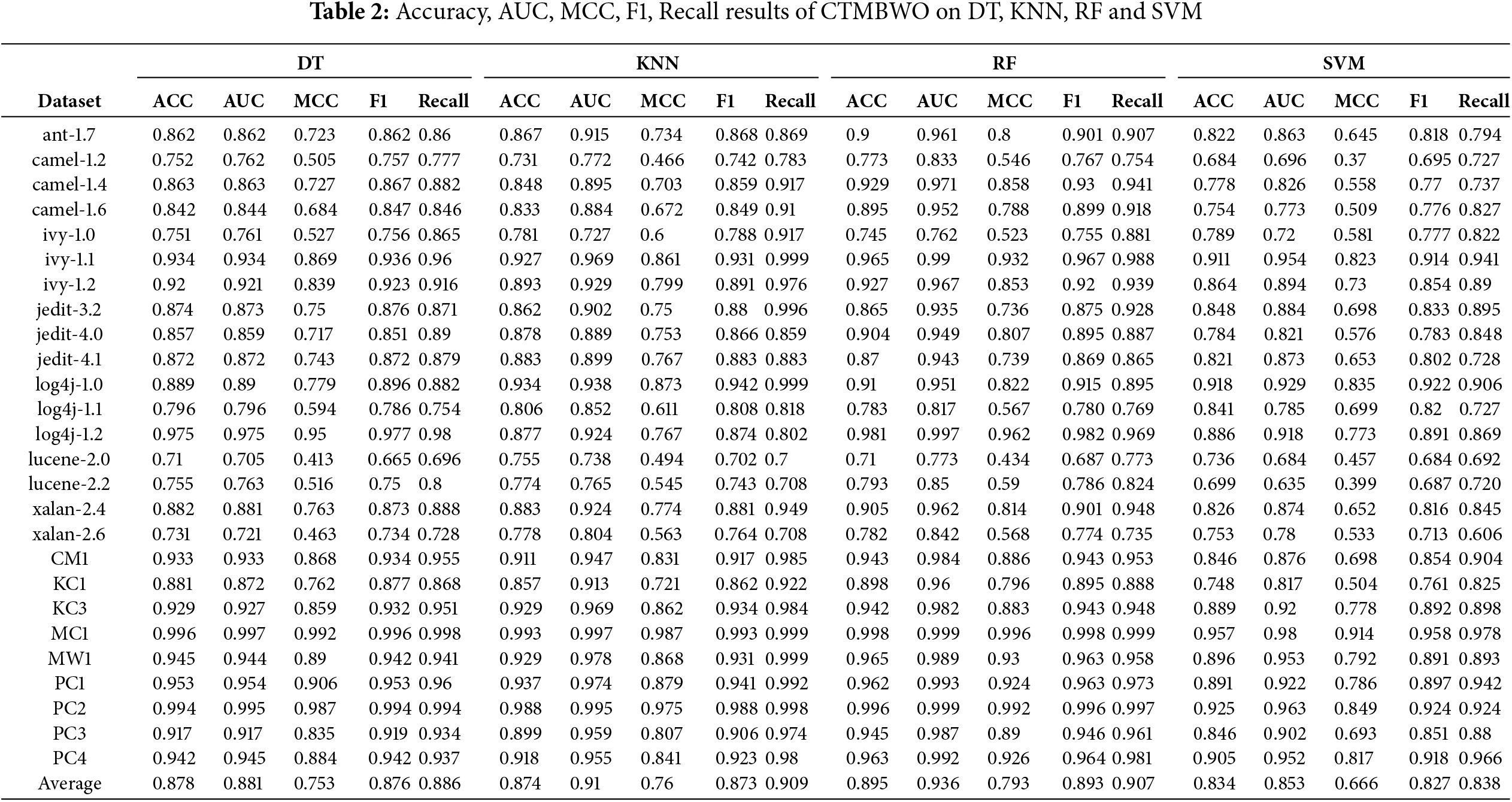
To evaluate the performance of CTMBWO, we use 5-fold cross-validation on four classifiers, namely SVM [25,26], RF [27], DT [28], and KNN [29], to conduct experiments and obtain the experimental results of Accuracy, AUC, MCC, F1, and Recall. Table 2 is the experimental results of the same version (training and testing are completed in the same project and the same version). Table 3 is the experimental results of the cross-version (Training is done with the lower version, and testing is conducted with the higher version).

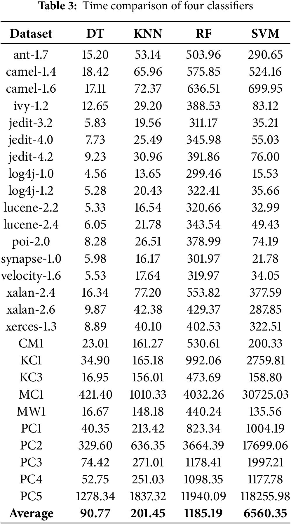
To further compare the performance of the four classifiers, we calculated their fitness values on several datasets, with the results shown in Fig. 4. And Table 4 presents the running time (in seconds) of the four classifiers after 100 iterations on each dataset, with the average value bolded.

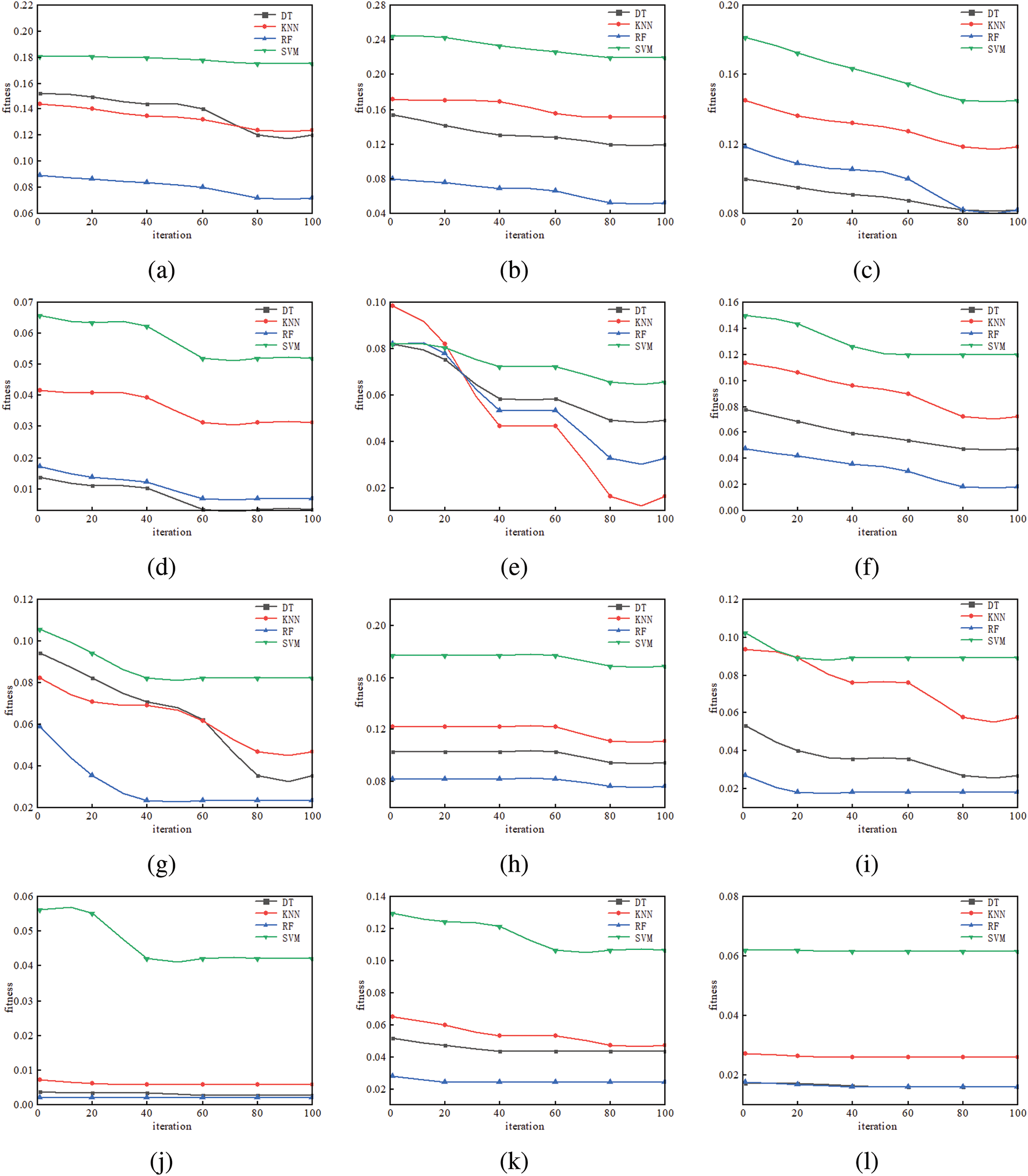
Figure 4: The fitness values of four classifiers on some datasets, (a) The fitness value of ant-1.7; (b) The fitness value of camel-1.4; (c) The fitness value of jedit-3.2; (d) The fitness value of jedit-4.3; (e) The fitness value of log4j-1.0; (f) The fitness value of poi-2.0; (g) The fitness value of synapse-1.0; (h) The fitness value of xalan-2.4; (i) The fitness value of MW1; (j) The fitness value of MC1; (k) The fitness value of PC1; (l) The fitness value of PC5

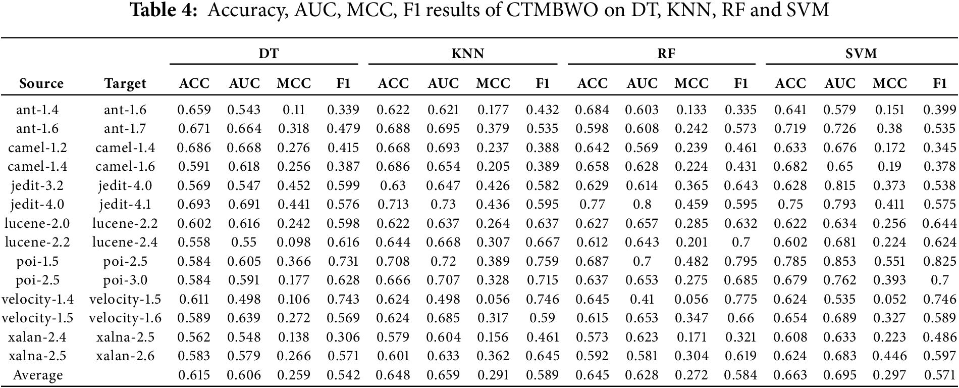
Table 2 illustrates that the experimental results obtained when using RF as a classifier are better than the other three classifiers. It can be concluded that the overall experimental results of projects Lucene and Log4j are worse than those of other projects; the overall experimental results of MC1 and PC2 are better than those of other projects. By specifically analyzing the detail of datasets in Table 1, projects MC1 and PC2 have 9466 and 5589 instances, respectively, while projects Lucene and Log4j have only 782 and 449 instances. From this, it is evident that the results of SD are closely linked to the number of instances in the project.

Table 4 shows that when using CTMBWO for cross-version defect prediction, the average accuracy is above 60%, the F1 value varies greatly for different projects, and the average MCC value is low, with the highest being 0.2963. It can be concluded that the prediction performance of using CTMBWO for cross-version prediction is weak. The main reason is that we only consider traditional features and do not further explore the semantic features and other dependencies between codes.

5.1 Comparison with Baseline Models

It can be concluded from Fig. 4 that the fitness values of the four classifiers are ranked as RF, DT, KNN, and SVM on most datasets. From Table 3, we observe that DT and KNN have the shortest running times among the classifiers. To further test the effectiveness of CTMBWO in feature selection, we compared CTMBWO with 4 prominent methods, namely GAPSO, Fed-OLF, MFWFS, and SLSTM. Table 5 shows a comparison between our method and the baseline methods(with the maximum value is bolded). Our results are the average of the outcomes obtained using KNN and RF as classifiers. And the comparison between CTMBWO and the baseline models’ average values is shown in Fig. 5. The ‘–’ in Table 5 indicates missing values, meaning there is no relevant data available in the original paper. We also attempted to reach out to the authors, but they did not share their code with us.

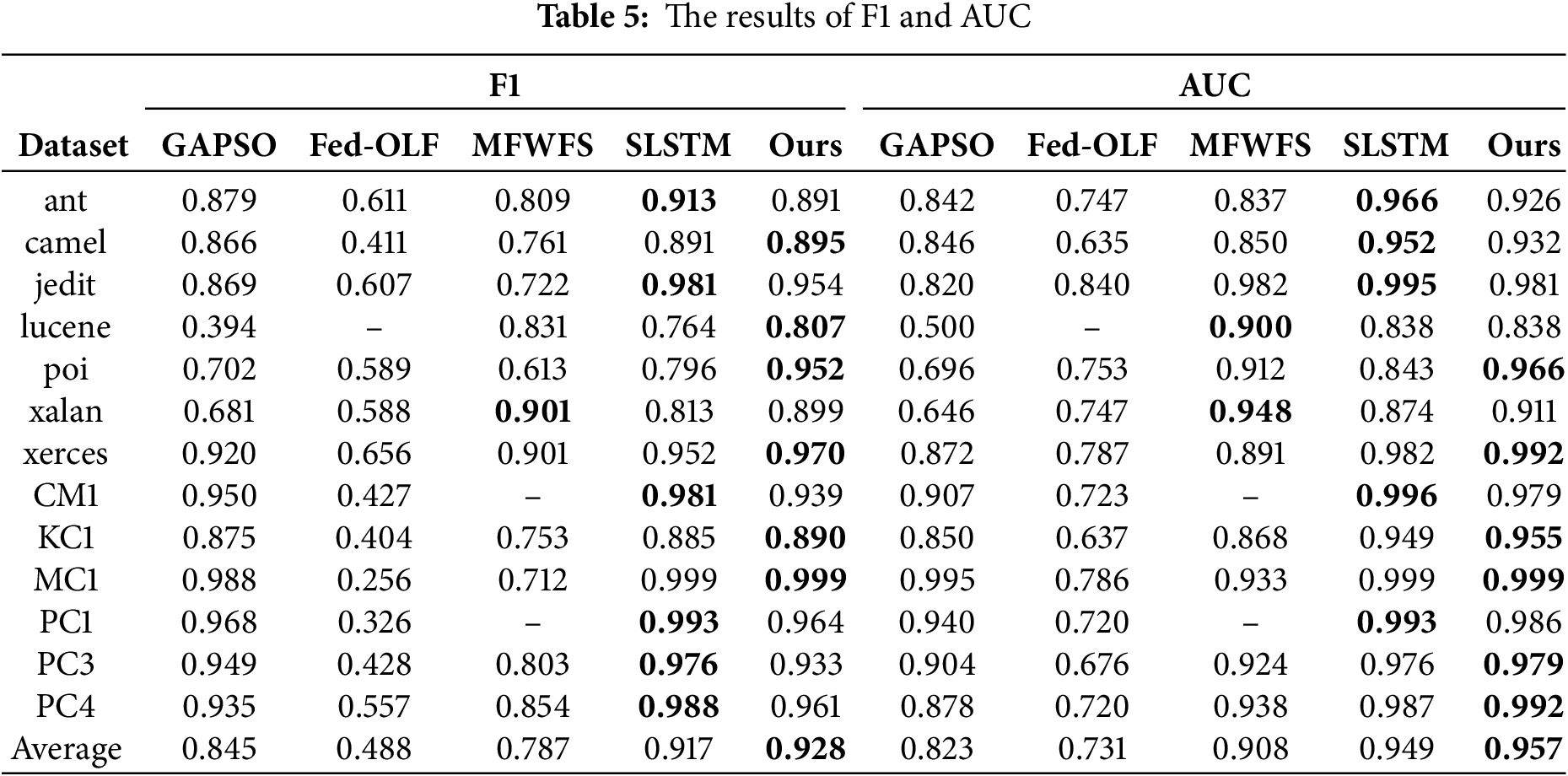
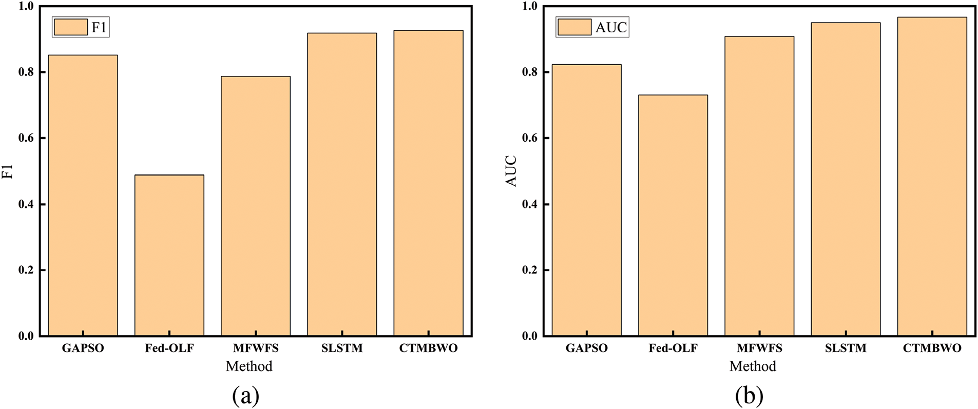
Figure 5: The comparison of the average values of F1 and AUC

Based on the results in Table 5, it can be observed that the F1 and AUC values of CTMBWO show significant improvements compared to the four baseline methods. The F1 score increased by 0.3%–74%, and AUC improved by 4.9%–33.8%. Additionally, the average F1 and AUC values of CTMBWO are higher than those of the baseline methods. These improvements indicate that CTMBWO is more effective at capturing the underlying patterns in the data, leading to higher accuracy and better performance in classification tasks. The increase in the F1 score suggests that the model performs better in handling class imbalance, achieving a better balance between recall and precision. The rise in AUC indicates that the model is more capable of distinguishing between different classes, especially when faced with complex and incomplete input data, making more accurate predictions. These results highlight the advantages of CTMBWO in defect prediction tasks and validate its effective improvement over baseline methods.

5.2 Ablation Experiment

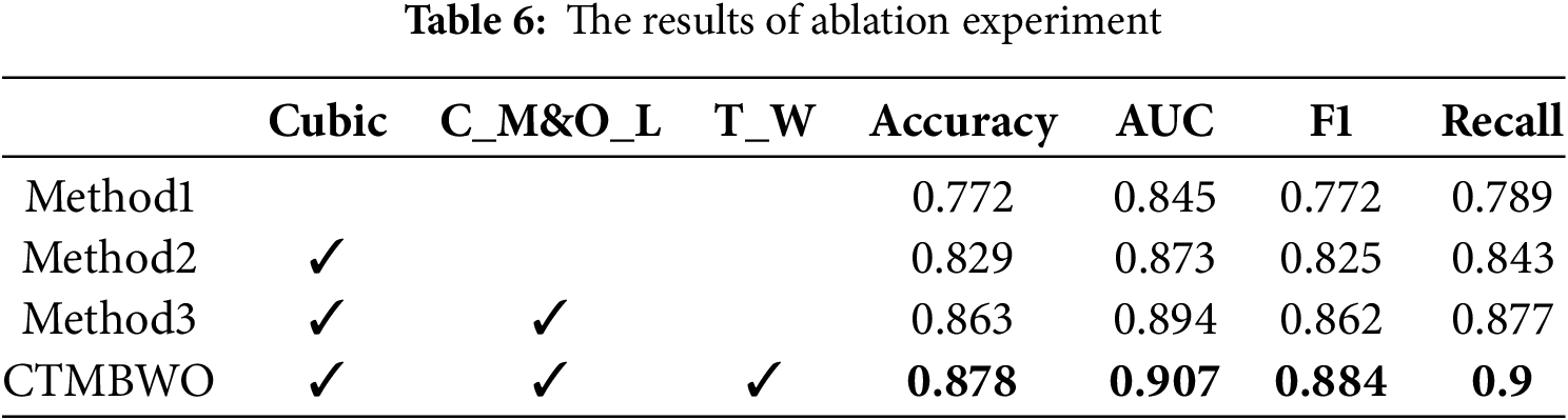
To further verifying the feasibility of our method, we conducted ablation experiments to compare the effects of using CTMBWO and other methods. Table 6 presents the results of ablation experiments. The methods tested include a baseline (Method1) without using feature selection, and two methods that incorporate Cubic chaotic mapping and an update mechanism combining Cauchy mutation and reverse learning. Method2 initializes the population using Cubic chaotic mapping, resulting in a 5.71% improvement in accuracy compared to Method1. Method3 builds on Method2 by adding a position update mechanism and achieves a further 3.46% improvement in accuracy. In Table 6, Cubic is the initialization of the population using Cubic chaotic mapping, C_M&O_L are the Cauchy variation and reverse learning, and T_W is the triangular wandering strategy.

In addition, we discussed the influence of parameters on the experimental results. The hyperparameter Tmax has minimal impact on the experimental results because we use the strategy of early stopping and cross validation to avoid overfitting. Therefore, we focus primarily on analyzing how the population size N affects the results. We set the population size to 10, 20, and 30 and the experimental results are shown in Table 7. From Table 7, we can see that as the population size increases, both the Accuracy and AUC values of the model generally improve. This suggests that a larger population size enhances the model’s performance. However, the population size cannot be increased indefinitely, as each individual in the population needs to be processed as the population grows, which significantly increases both computational time and space complexity, and may slow down the speed of convergence. In other words, the algorithm will take longer to reach the optimal solution. For this reason, we chose a population size of 30, which strikes a balance between resource usage and model performance.

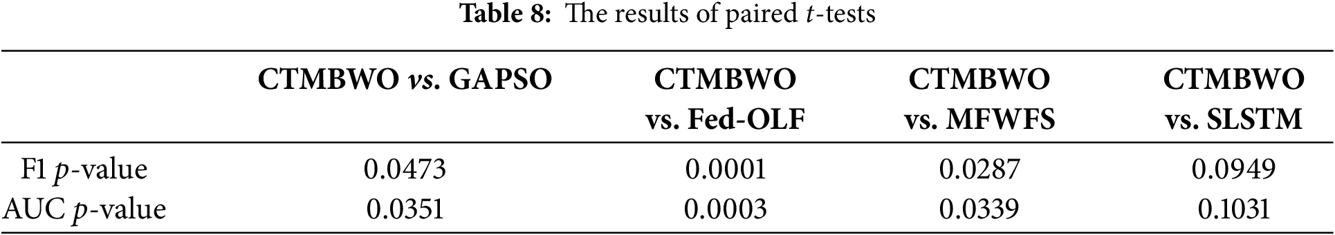
5.3 The results of Paired t-Tests

Table 8 summarizes the results obtained from the paired t-test at a significance level of 5%. The results show that CTMBWO significantly outperforms the three baseline models: GAPSO, Fed-OLF and MFWFS. Although the significance of CTMBWO compared to SLSTM is not as pronounced, we can conclude from the comparison of the average values in Table 5 and Fig. 5 that CTMBWO’s classification performance is clearly superior to that of SLSTM.

6  Conclusion and Future Work

This study proposes a new feature selection method CTMBWO to effectively select the optimal feature subset. CTMBWO aims to exclude redundant and irrelevant features and thus select the most important features. We evaluated the performance of CTMBWO on 19 project using four classifiers and compared the performance with existing models. The results demonstrate that applying CTMBWO in feature selection significantly enhances the performance of SDP. Specifically, the average F1 value increases by 74%, the average AUC value increases by 33.8%. These improvements show that the algorithm effectively removes redundant and irrelevant features and selects the most valuable features for defect prediction, thereby enhancing the accuracy of the model. Furthermore, the CTMBWO improves population diversity and global search capabilities, effectively avoids local optimal solutions, and thus improves the prediction effect.

The application scenarios of CTMBWO in feature selection problems in machine learning include medical diagnosis, image processing, financial analysis, and text classification. Feature selection helps identify key indicators that are most relevant to the task, improving disease prediction accuracy, enhancing classification precision, optimizing risk assessment and investment decisions, and boosting text classification effectiveness.

However, CTMBWO has some limitations. It mainly performs feature selection based on traditional features and cannot consider the semantic information between codes, which leads to poor performance when predicting cross-version defect prediction. Therefore, future research will focus on exploring methods that combine semantic information and traditional features for SDP.

Acknowledgement: We are grateful to our families and friends for their unwavering understanding and encouragement.

Funding Statement: Not applicable.

Author Contributions: The authors confirm contribution to the paper as follows: study conception and design: Shaoming Qiu, Jingjie He, Yan Wang and Bicong E; data collection and analysis: Shaoming Qiu, Jingjie He and Bicong E; draft manuscript preparation: Shaoming Qiu and Jingjie He. All authors reviewed the results and approved the final version of the manuscript.

Availability of Data and Materials: The data that support the findings of this study are available from the corresponding author, Yan Wang, upon reasonable request.

Ethics Approval: Not applicable.

Conflicts of Interest: The authors declare no conflicts of interest to report regarding the present study.

References

1. Pachouly J, Ahirrao S, Kotecha K, Selvachandran G, Abraham A. A systematic literature review on software defect prediction using artificial intelligence: datasets, data validation methods, approaches, and tools. Eng Appl Artif Intell. 2022;111:104773. doi:10.1016/j.engappai.2022.104773. [Google Scholar] [CrossRef]

2. Goyal S, Bhatia PK. Comparison of machine learning techniques for software quality prediction. Int J Knowl Syst Sci. 2020;11(2):20–40. doi:10.4018/IJKSS. [Google Scholar] [CrossRef]

3. Pal S, Sillitti A. Cross-project defect prediction: a literature review. IEEE Access. 2022;10:118697–717. doi:10.1109/ACCESS.2022.3221184. [Google Scholar] [CrossRef]

4. Zhao Y, Damevski K, Chen H. A systematic survey of just-in-time software defect prediction. ACM Comput Surv. 2023;55(10):1–35. doi:10.1145/3567550. [Google Scholar] [CrossRef]

5. Goyal S, Bhatia PK. Software fault prediction using lion optimization algorithm. Int Inf Technol. 2021;13:2185–90. doi:10.1007/s41870-021-00804-w. [Google Scholar] [CrossRef]

6. Malhotra R, Khan K. A novel software defect prediction model using two-phase grey wolf optimisation for feature selection. Cluster Comput. 2024;1–23. doi:10.1007/s10586-024-04599-w. [Google Scholar] [CrossRef]

7. Chantar H, Mafarja M, Alsawalqah H, Heidari AA, Aljarah I, Faris H. Feature selection using binary grey wolf optimizer with elite-based crossover for Arabic text classification. Neural Comput Appl. 2020;32:12201–20. doi:10.1007/s00521-019-04368-6. [Google Scholar] [CrossRef]

8. Goyal S. Genetic evolution-based feature selection for software defect prediction using SVMs. J Circuits Syst Comput. 2022;31(11):2250161. doi:10.1142/S0218126622501614. [Google Scholar] [CrossRef]

9. Das H, Prajapati S, Gourisaria MK, Pattanayak RM, Alameen A, Kolhar M. Feature selection using golden jackal optimization for software fault prediction. Mathematics. 2023;11(11):2438. doi:10.3390/math11112438. [Google Scholar] [CrossRef]

10. Arasteh B, Arasteh K, Ghaffari A, Ghanbarzadeh R. A new binary chaos-based metaheuristic algorithm for software defect prediction. Cluster Comput. 2024;1–31. doi:10.1007/s10586-024-04486-4. [Google Scholar] [CrossRef]

11. Kukkar A, Kumar Y, Sharma A, Sandhu JK. Bug severity classification in software using ant colony optimization based feature weighting technique. Expert Syst Appl. 2023;230:120573. doi:10.1016/j.eswa.2023.120573. [Google Scholar] [CrossRef]

12. Anbu M, Anandha Mala G. Feature selection using firefly algorithm in software defect prediction. Clust Comput. 2019;22:10925–34. doi:10.1007/s10586-017-1235-3. [Google Scholar] [CrossRef]

13. Wang H, Arasteh B, Arasteh K, Gharehchopogh FS, Rouhi A. A software defect prediction method using binary gray wolf optimizer and machine learning algorithms. Comput Electr Eng. 2024;118:109336. doi:10.1016/j.compeleceng.2024.109336. [Google Scholar] [CrossRef]

14. Sekaran K, Lawrence SPA. Mutation boosted salp swarm optimizer meets rough set theory: a novel approach to software defect detection. Trans Emerg Telecomm Technol. 2024;35(3):e4953. doi:10.1002/ett.4953. [Google Scholar] [CrossRef]

15. Alsghaier H, Akour M. Software fault prediction using particle swarm algorithm with genetic algorithm and support vector machine classifier. Softw Pract Exp. 2020;50(4):407–27. doi:10.1002/spe.2784. [Google Scholar] [CrossRef]

16. Feng J, Zhang J, Zhu X, Lian W. A novel chaos optimization algorithm. Multimed Tools Appl. 2017;76:17405–36. doi:10.1007/s11042-016-3907-z. [Google Scholar] [CrossRef]

17. Zhong C, Li G, Meng Z. Beluga whale optimization: a novel nature-inspired metaheuristic algorithm. Knowl Based Syst. 2022;251(1):109215. doi:10.1016/j.knosys.2022.109215. [Google Scholar] [CrossRef]

18. Mantegna RN. Fast, accurate algorithm for numerical simulation of Levy stable stochastic processes. Phys Rev E. 1994;49(5):4677. doi:10.1103/PhysRevE.49.4677. [Google Scholar] [PubMed] [CrossRef]

19. Ryu D, Choi O, Baik J. Improving prediction robustness of VAB-SVM for cross-project defect prediction. In: 2014 IEEE 17th International Conference on Computational Science and Engineering; 2014; Sanya, China: IEEE. p. 994–9. doi:10.1109/CSE.2014.198. [Google Scholar] [CrossRef]

20. Fenton N, Bieman J. Software metrics: a rigorous and practical approach. CRC Press; 2014. [Google Scholar]

21. Fernández A, Garcia S, Herrera F, Chawla NV. SMOTE for learning from imbalanced data: progress and challenges, marking the 15-year anniversary. J Artif Intell Res. 2018;61:863–905. doi:10.1613/jair.1.11192. [Google Scholar] [CrossRef]

22. Hu X, Zheng M, Zhu R, Zhang X, Jin Z. Fed-OLF: federated oversampling learning framework for imbalanced software defect prediction under privacy protection. IEEE Trans Reliab. 2025. doi:10.1109/TR.2024.3524064. [Google Scholar] [CrossRef]

23. Malhotra R, Chawla S, Sharma A. Software defect prediction based on multi-filter wrapper feature selection and deep neural network with attention mechanism. Neural Comput Appl. 2025;2025:1–28. doi:10.1007/s00521-024-10902-y. [Google Scholar] [CrossRef]

24. Vasishth O, Bansal A. Enhanced software defect prediction using krill herd algorithm with stacked LSTM with attention mechanism. Int J Syst Assur Eng Manag. 2024;2024:1–21. doi:10.1007/s13198-024-02630-2. [Google Scholar] [CrossRef]

25. Weston J, Mukherjee S, Chapelle O, Pontil M, Poggio T, Vapnik V. Feature selection for SVMs. Adv Neural Inf Process Syst. 2000; 647–53. doi:10.5555/3008751.3008845. [Google Scholar] [CrossRef]

26. Nguyen MH, De la Torre F. Optimal feature selection for support vector machines. Pattern Recognit. 2010;43(3):584–91. doi:10.1016/j.patcog.2009.09.003. [Google Scholar] [CrossRef]

27. Breiman L. Random forests. Mach Learn. 2001;45:5–32. doi:10.1023/A:1010933404324. [Google Scholar] [CrossRef]

28. Krawczyk B, Woźniak M, Schaefer G. Cost-sensitive decision tree ensembles for effective imbalanced classification. Appl Soft Comput. 2014;14:554–62. doi:10.1016/j.asoc.2013.08.014. [Google Scholar] [CrossRef]

29. Meiliana, Karim S, Warnars HLHS, Gaol FL, Abdurachman E, Soewito B. Software metrics for fault prediction using machine learning approaches: a literature review with PROMISE repository dataset. In: 2017 IEEE International Conference on Cybernetics and Computational Intelligence (CyberneticsCom); 2017; Exeter, UK: IEEE. p. 19–23. doi:10.1109/CYBERNETICSCOM.2017.8311708. [Google Scholar] [CrossRef]