Rolling Bearing Fault Diagnosis Based on Cross-Attention Fusion WDCNN and BILSTM

1  Introduction

The reliability of high-speed train engines plays a key role in ensuring the normal operation of trains, and rolling bearings are integral components of high-speed train engines, providing support for rotating parts and reducing friction as well as bearing loads [1]. However, bearing damage can occur due to overloading, overheating, normal fatigue failure, contamination, lubricant failure, and corrosion [2]. Fault diagnosis, as an important method of monitoring the condition of bearings [3], can detect failures in time, thus preventing unnecessary losses due to bearing damage.

In bearing fault diagnosis technology, vibration signals have become the most commonly used monitoring indicators, and the majority of common faults can be identified through the analysis of vibration signals. However, usually due to the complexity of the environment, the collected vibration signals present a nonlinear and non-stationary state, so signal processing has become an inevitable step [4–7]. The most commonly employed signal processing techniques encompass time-domain analysis, frequency-domain analysis, and time-frequency domain analysis. The latter has gained considerable traction due to its capacity to encapsulate both temporal and spectral attributes [8]. Among the most commonly employed time-frequency domain analysis methods, the VMD [9] has a good concentration in the time-frequency domain because of its (1) powerful time-frequency decomposition capability, which can decompose a complex signal into several intrinsic modal functions (IMFs) with finite bandwidth [10]. Compared with the traditional empirical modal decomposition (EMD), VMD introduces a frequency domain optimization model in the decomposition process to avoid the modal aliasing problem of EMD [11]. (2) Nonlinear and non-smooth signal analysis. For nonlinear and nonsmoothed signals, it may be difficult to obtain good time-frequency analysis by traditional methods, and the bandwidth optimization mechanism of VMD can effectively handle such signals [12]. (3) Noise reduction and feature extraction, when processing signals containing noise, VMD can separate the noise component from the main signal component, which facilitates the retention of signal features [13]. By analyzing the time-frequency characteristics of the decomposed modes [14], important information in specific frequency bands can be extracted. In summary, because VMD has the above ability to process signals, it has a wide range of applications in the field of signal processing.

The advent of deep learning as a computational framework has led to the emergence of numerous sophisticated deep learning algorithms in the field of fault diagnosis [15–17]. Convolutional neural network (CNN) [18], as a classical deep neural network, has been extensively employed in the domains of lifetime prediction and fault diagnosis. Literature [19] proposed a stacked CNN-based multiscale feature extraction scheme to improve the accuracy of the model. Literature [20] uses the acquired vibration signals directly as inputs to the CNN, resulting in end-to-end fault diagnosis. However, the above algorithm ignores the effect of noise on diagnosis. Literature [21] proposes a first-layer wide convolutional kernel neural network that achieves an accuracy of more than 90% at a signal-to-noise ratio of −4 dB, which results in a model that possesses strong performance even under strong noise. To address the issue of long-term information dependence, two types of neural networks have been proposed: the LSTM and the BILSTM. Literature [22] used LSTM models to analyze fault characteristics in motor current signals and achieved efficient diagnosis of rolling bearing faults by capturing the time series relationship of current signals. Literature [23] proposed an improved bidirectional LSTM neural network model to enhance the accuracy of fault classification by combining forward and backward time series characteristics. Literature [24] proposes a new multi-scale wide convolutional kernel convolutional neural network for bearing fault diagnosis, aiming to enhance the model’s ability to extract features of different scales by introducing convolutional kernels of different sizes, to improve the accuracy. In the literature [25], a multi-scale convolution kernel network is used to capture fault features of different scales, and LSTM is used to model the time series characteristics of fault signals, to achieve accurate diagnosis of different fault modes.

In recent years, the combination of attentional mechanisms and neural networks has become a megatrend with a wide range of applications in the field of mechanical fault diagnosis. The core idea of the attention mechanism is to mimic the human vision and attention system by focusing on important information and ignoring secondary information [26]. It enables the model to process complex data more efficiently by dynamically assigning weights to different parts of the input. Literature [27] proposes an attention-based bilinear feature fusion method, by fusing features from multiple signals, the model can better extract complementary fault information, while the cross-attention mechanism is used to dynamically adjust the feature weights to improve the diagnostic performance. Literature [28] proposes a bearing fault diagnosis method that combines CNN and attention mechanism, automatically extracts features through visual vibration signal analysis, and uses the attention mechanism to highlight important information in fault signals. Literature [29] proposes a twin converter model based on cross-attention fusion, which can improve the model’s ability to recognize complex fault modes by simultaneously processing features in the time domain and frequency domain and carrying out feature fusion across attention mechanisms.

The WDCNN can automatically extract the spatial features from the signals, but it is less capable of processing time-series data with strong time dependence, while the BILSTM effectively solves the long-term dependency problem. Therefore, by combining the two, it is possible to enhance the extraction of spatial and time-sequence features, thus obtaining more comprehensive information about the signal. Cross-attention mechanism, on the other hand, enables feature fusion by exploiting the correlation between two input features (Query and Key-Value).

Combining the above theories, rolling bearing fault diagnosis based on cross-attention fusion of WDCNN and BILSTM is proposed. It not only gives full play to the respective advantages of WDCNN and BILSTM networks but also achieves feature complementarity. Moreover, the signal is preprocessed using VMD decomposition to reduce the burden of the neural network, enhance the performance of the model, and improve the accuracy. The model proposed in this paper addresses the limitations imposed by the single-feature extraction method in the domain of bearing fault diagnosis. It employs a dynamic feature fusion approach to address the issue of model instability caused by a single feature. The validity of this approach is substantiated by experimental findings that demonstrate enhanced accuracy and reliability in comparison to conventional models.

2  Methods

2.1 Variational Modal Decomposition

VMD is an adaptive time-frequency analysis method based on signal decomposition. VMD is capable of decomposing complex signals into a number of modes (IMFs) and can handle non-stationary signals efficiently. The core idea of VMD decomposition is to decompose the signal by finding the center frequency of the components and bandwidth minimization.

The goal of the VMD is to minimize the objective function of Eq. (1):

min{uk,ωk}∑k‖∂t[(δ(t)+jπt)uk(t)]e−jwkt‖22(1)

where, ωk represents the center frequency of each mode, (δ(t)+jπt)uk(t) is the Hilbert transform of uk(t), It is used to extract the positive frequency part of the signal.

The constraints on the objective function are:

f(t)=∑K=1Kuk(t)(2)

where, K stands for the number of components.

The constraints mean that the sum of all components can reconstruct the original signal.

Variational solution process: the constrained optimization is converted to unconstrained optimization by α and a Lagrange function.

Lagrange function:

L({uk},{ωk},λ)=α∑k‖δt[(δ(t)+jπt)uk(t)]e−jwkt‖22+‖f(t)−∑kuk(t)‖22+<λ(t),f(t)−∑kuk(t)>(3)

Iterative update: Iterative solution by alternating direction multiplier method as a way to update uk, ωk and λ.

Update the modal component uk:

ukn+1(ω)=f(ω)−∑i≠kui(ω)+λ(ω)21+2α(ω−ωk)2(4)

Frequency of updating centers ωk:

ωkn+1=∫0∞ω|uk(ω)|2dω∫0∞|uk(ω)|2dω(5)

Updating Lagrange multipliers λ:

λn+1(ω)=λn(ω)+τ(f(ω)−∑kukn+1(ω))(6)

Repeat (3)–(6) and the VMD iteration stops when the decomposed modes satisfy the following equation:

∑k‖ukn+1−ukn‖22/∑k‖ukn‖22<ϵ(7)

The decomposition can be completed through the above process, and VMD decomposition has the following advantages: adaptive (no need to preset the decomposition bandwidth, and can automatically adjust the decomposition bandwidth and center frequency of the signal), highly robust (compared with empirical modal decomposition, VMD is more robust to the noise, and avoids the problem of mode aliasing), and controllable (by adjusting the parameter α and the number of decomposed modes K, the accuracy and effect of decomposition can be controlled), and so on.

2.2 WDCNN Network

CNN is nowadays widely used in the fields of image processing, natural language recognition, etc., and has now been widely used in the field of bearing fault diagnosis. CNN consists of input, convolution, activation, pooling, fully connected, and output layers. There are some shortcomings of convolutional neural networks, for example, when dealing with one-dimensional vibration signals, unlike 2D images, where CNNs perform well with small 3 × 3 kernels on 224 × 224 images, it is impractical to design a model using only 3 × 1 small kernels for 1D vibration signals, such as 1024 × 1 or 2048 × 1 sequences. This would result in a very deep network and difficult to train. In addition, the small kernels in the initial layer are vulnerable to disruption from high-frequency noise, which is prevalent in industrial settings. It is therefore necessary to capture useful information about the vibration signals in the low and medium frequency bands and to process one-dimensional signals optimally, the first layer of convolution uses a wide convolution kernel to extract the features, and then successively smaller 3 × 1 kernels are used to obtain a better representation of the features, and the structure of the model is shown in Fig. 1.

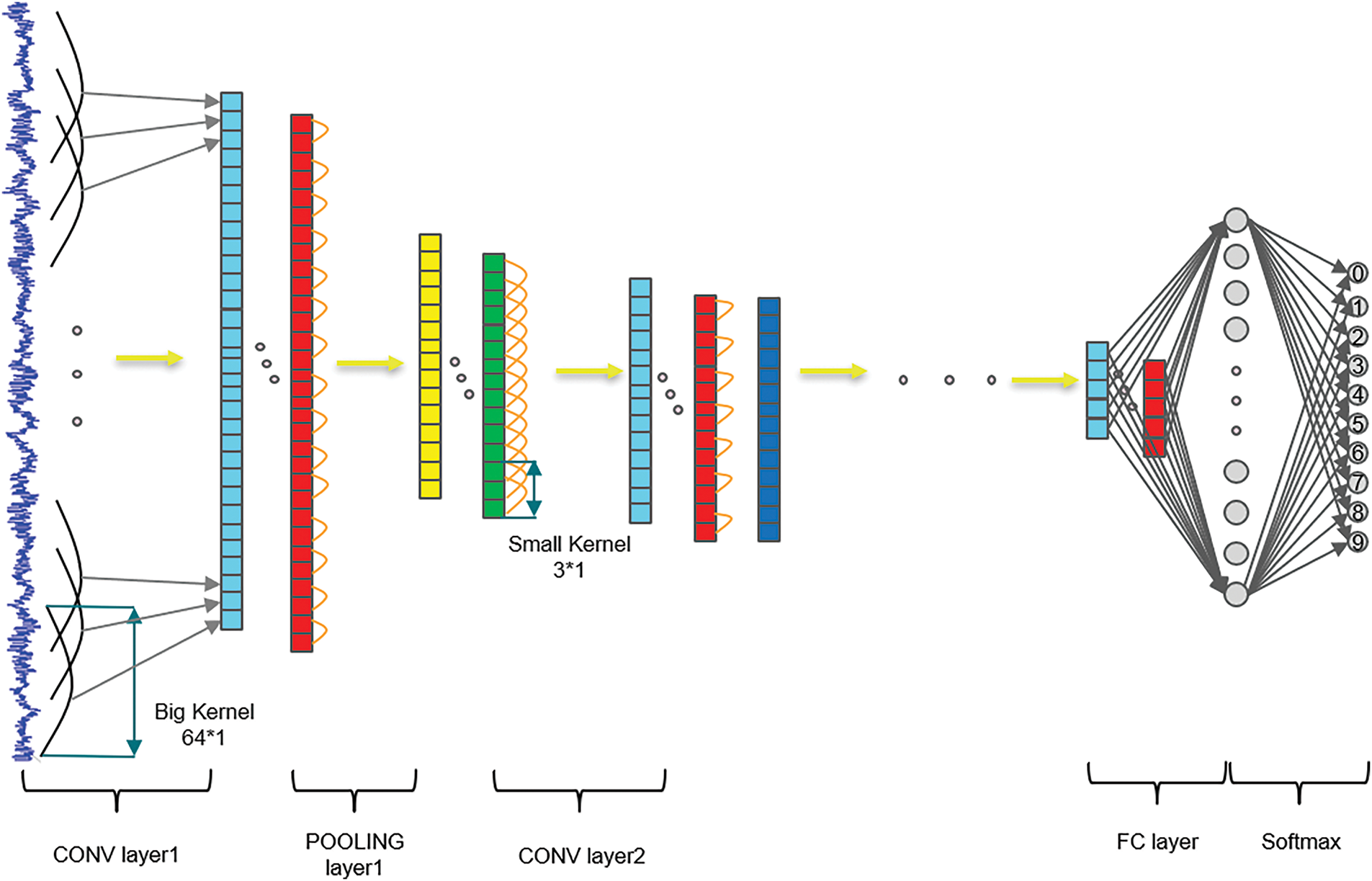
Figure 1: WDCNN model

WDCNN is generally an extension of traditional CNN, because the first layer is a convolutional layer with a wide convolutional kernel and has multiple convolutional layers, so the feature extraction effect of the vibration signal is improved. It can directly process one-dimensional signals, avoiding the loss of features due to other transformations, and the extensive convolution kernel utilized in the initial layer is capable of effectively mitigating the adverse effects of high-frequency noise, which is more conducive to capturing useful information in the low and medium frequency vibration signals.

2.3 BILSTM Network

In order to be able to adequately capture the time-series characteristics of vibration signals, a BILSTM is therefore used. Compared with the traditional LSTM, the BILSTM [30] consists of a combination of a forward LSTM [31] and a backward LSTM, and thus it can not only learn the information before the current moment but also make use of the information afterward.

The structure of BILSTM is shown in Fig. 2. In BILSTM, the input data goes into two LSTM layers, respectively. Two LSTM layers: one is a forward pass layer, which is used to train the forward time series. One is the backward pass layer, which is used to train the backward time series. The pre-passing and post-passing layers have the same composition and work on the same principle, except that the input sequences are in reverse order. The outputs of the two layers are connected and finally output by integration.

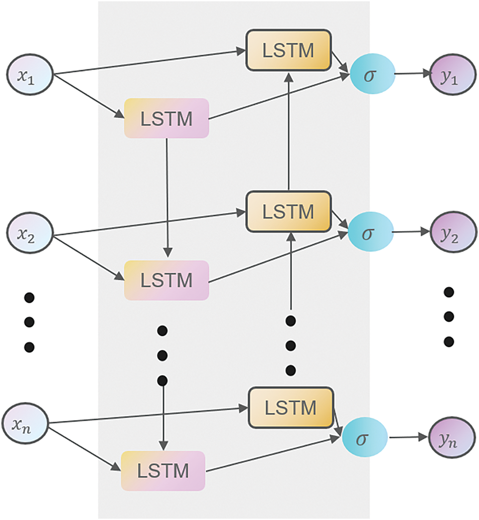
Figure 2: BILSTM model structure

The LSTM component of the BILSTM structure represents an advancement over the Recurrent Neural Network (RNN). As illustrated in Fig. 3, the LSTM structure addresses the issue of gradient vanishing and exploding during the training process by incorporating input gates, forgetting gates, output gates, and memory units.

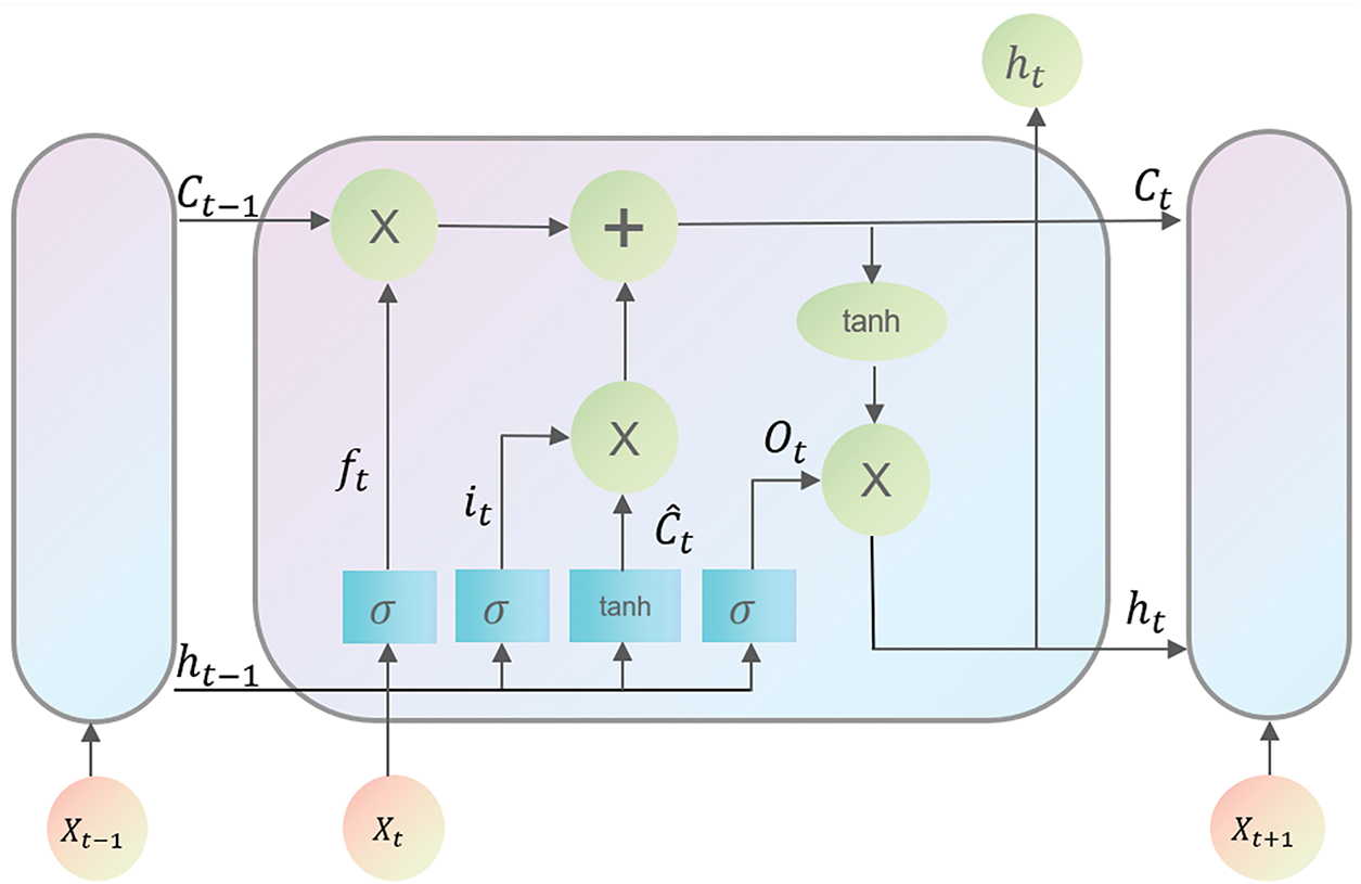
Figure 3: LSTM model structure

The idea of LSTM calculation is as follows:

Oblivion gate: determines how much of the information delivered in the previous time step is discarded.

ft=σ(Wf⋅[ht−1,xt]+bf)(8)

where, xt is the input of the current time step, ht−1 is the hidden state of the previous time step.

Input gate: determines the quantity of information entered at the current time step that can be written to the cell state.

it=σ(Wi⋅[ht−1,xt]+bi)(9)

C~t=tanh(Wc⋅[ht−1,xt]+bc)(10)

where, C~t is the temporary cell state, σ and tanh are the activation functions.

Memory unit: carries memory information for long time sequences, it is the core of LSTM.

Ct=ft⋅Ct−1+it⋅C~t(11)

where, Ct−1 is the cell state at the previous moment, Ct is the cell state at the current moment.

Output Gate: determines how much of the current time’s output is used as a hidden state.

ot=σ(Wo⋅[ht−1,xt]+bo)(12)

ht=ot⋅tanh⁡(Ct)(13)

where, ot represents the value of the output gate, ht is the current hidden state.

2.4 Cross-Attention Mechanisms

Cross-Attention Mechanism (CAM) is an important technique used for multi-input sequence processing, aiming at extracting the relationship between two or more features through mutual correlation operations. The core idea is to match a set of queries (Query) with another set of keys (Key) and values (Value) to extract the relevant information of both.

Cross-attention mechanisms differ from general self-attention mechanisms in that they deal with features from different sources or different representations and are therefore more suitable for related tasks such as feature fusion.

The formula is expressed as:

1.    First assume that two sets of features are input:

(a)    Query the feature matrix Q∈RLQ×d.

(b)    Key identity matrix K∈RLK×d and value identity matrix V∈RLK×d.

Weighting of attention: dot product calculation by K and V, with scaling and normalization.

AttentionWeights(Q,K)=softmax(QKTd)(14)

where, QKT∈RLQ×LK denotes the relevance of the query and key, and d is the scaling factor.

Calculation of weighted sums: Based on the above weights, V is weighted and summed.

CrossAttention(Q,K,V)=AttentionWeights(Q,K)V(15)

The final output of the cross-attention is obtained: it results in a new feature matrix of dimension RLQ×d.

Output=oftmax(QKTd)V(16)

The cross-attention mechanism is characterized by dynamic mapping between one set of inputs and another set of inputs, which can effectively capture the interaction between different modes or feature sources. In comparison with alternative attention mechanisms, it possesses the following advantages: (1) Focus on multi-modal fusion: This makes it a better fit for the multi-source feature fusion needs of this study. (2) Enhance feature complementarity: Exploration of the correlation between different features is facilitated by the dynamic interaction of Query and Key/Value. (3) High computational efficiency: In comparison with global attention, cross attention merely necessitates the calculation of the weight matrix between cross-sources, thus resulting in reduced computational complexity. Consequently, this paper elects the cross-attention mechanism as the method for feature fusion.

2.5 Model Architecture

Based on the above theory, the model structure of this paper is proposed, based on the cross-attention fusion of WDCNN and BILSTM for the rolling bearing diagnosis model. The model structure is shown in Fig. 4.

Figure 4: Model structure diagram

The diagnostic idea mainly includes the following. Firstly, the vibration signals were decomposed by VMD, and multiple IMF components were obtained after decomposition, calculating the envelope entropy and kurtosis values for each component (The smaller the envelope entropy value means the higher the correlation of the component, the more faults it contains. Kurtosis [32] is an index that describes the spikiness of the waveform, according to the value of the kurtosis under normal conditions, the value of the kurtosis approximately obeys the normal distribution close to 3, when the bearing fails, and the kurtosis value of the fault signal will increase, so the larger the value of the kurtosis indicates that the more shock components are contained in the component). The components that conform to both envelope entropy and crag are filtered out and reconstructed, thus completing the initial noise reduction of the signal and retaining the main fault characteristic components.

The subsequent stage of the process involves the input of the reconstructed signals into the WDCNN and BILSTM networks, respectively, to extract different features of the signals. The first layer of the WDCNN uses a wide convolution kernel, which can capture the characteristic pattern of the signal more efficiently while carrying out high-frequency noise reduction. In comparison with a small convolution kernel, a wide convolution kernel demonstrates superiority in terms of its ability to capture features during the extraction process. The spatial feature of the signal is extracted in the WDCNN network. The BILSTM network utilized in this study comprises two layers: the first layer incorporates 32 hidden units, while the second layer comprises 64 hidden units. The activation function employed in the hidden layer is the hyperbolic tangent function (Tanh). The BILSTM network is primarily employed to capture the temporal relationship that exists within the feature sequence. The bi-directional LSTM structure enables the model to learn both forward and backward dependencies of the sequence data, thereby facilitating a comprehensive understanding of the dynamic features inherent in time series data.

Finally, the spatial features extracted by WDCNN and the temporal features extracted by BILSTM are, respectively, input into the cross-attention module for fusion. In this process, the features extracted by WDCNN are regarded as Query, and the features extracted by BILSTM are regarded as Key and Value, respectively. The output of the two is weighted by the cross-attention mechanism. The cross-attention mechanism can dynamically adjust the weights of WDCNN and BILSTM output according to the current input features. This enables the model to automatically optimize the feature selection under different input signals, thus improving the diagnostic accuracy. The fused features are then sent to the Fully Connected Layer for classification, which ultimately enables the diagnosis and classification of different fault types. The architecture of the model is such that WDCNN captures local spatial information, while BILSTM addresses the time dependence of these local features. Ultimately, the combination of time domain information and frequency domain information facilitates a more accurate classification of bearing fault signals.

3  Model Testing

The proposed model in this paper is tested using the public dataset provided by Case Western Reserve University (CWRU).

3.1 Data Set and Segmentation

The data were obtained from the Bearing Test Centre of CWRU, using deep groove ball bearings of model SKF 6205, which were experimentally obtained after manufacturing faults by EDM. The vibration signals were collected from the drive end of the experimental bench with a motor speed of 1772 r/min, a load of 1 HP, and a sampling frequency of 12 kHz.

The data set used in this paper includes normal, inner ring failure, rolling body failure, and outer ring failure in a total of four states, and each failure state also includes: 0.1778, 0.3556, 0.5334 mm three failure levels represent light to medium-heavy failures, so the sample data contains a total of ten failure states, the specifics are shown in Table 1.

The sample length of each data set is 1024, and the data are expanded by overlapping sampling with an overlap ratio of 0.5, and the division is shown in Fig. 5. The data are divided into a training set, validation set, and test set in the ratio of 0.7, 0.2 and 0.1. In summary, there are 10 states and 2330 data samples, and the training set contains 1631 samples, the validation set contains 466 samples, and the test set contains 233 samples.

Figure 5: Overlapping sample division

3.2 Signal Pre-Processing

In this paper, noise reduction is performed by VMD, and the choice of K and α as the main parameters is particularly important. K determines the number of components of VMD decomposition. In rolling bearing fault signal processing, different fault types usually correspond to characteristic signals in different frequency bands. Combined with experience and signal spectrum analysis, the four modes can cover the main characteristic frequencies while avoiding redundancy or overfitting problems caused by too many components. α controls the convergence of the decomposition process and the sparsity of the modes. According to the literature [33] and our analysis of bearing signals, α = 2000 can effectively separate different modes in a noisy environment, while ensuring the stability and physical meaning of the decomposition results. After the VMD decomposition, four IMF components are obtained, and then the entropy of the envelope (It has been established that an increase in the value of the envelope entropy is indicative of a more complex change in the signal. This is most commonly related to the instability or fault state of the system. By comparing the envelope entropy in different states, the health status of the device can be determined) and the kurtosis value (This statistic is employed to describe the distribution pattern of a signal or data set. It is typically utilized to assess the degree of concentration present in a signal’s tail distribution, relative to the parameters of a normal distribution. The term “spiky” is often used to describe a signal with a pronounced tail distribution, characterized by its high concentration of data points) of the four components are computed, and the IMF components with smaller entropy and larger kurtosis are filtered out and reconstructed to obtain the signal after noise reduction. Components with small envelope entropy values and large kurtosis values are filtered out and reconstructed to obtain the noise-reduced signal.

To show the signal processing process more clearly, the signal with serial number 4 in Table 1, the fault diameter of 0.5334 mm, and the fault type of the inner ring fault is shown as an example. First of all, the VMD decomposition of the fault signal to obtain its decomposition of the time domain signal map shown in Fig. 6.

Figure 6: Decomposition time-domain diagram

After obtaining the four IMF components continue to calculate the envelope entropy value and the kurtosis value of each component, the kurtosis is defined as follows, the particular outcomes are presented in Table 2, and the signal components that meet the screening conditions are selected for reconstruction.

K=E(x−μ)4σ4(17)

From Table 2, it can be seen that the envelope entropy values of components 3 and 4 are smaller than the other components, while the kurtosis values are also significantly larger than the other components, so it is more helpful for the next diagnosis to include a large amount of information about the original signal in components 3 and 4, and therefore, components 3 and 4 are selected for the reconstruction of the signal.

The reconstructed signal is shown in Fig. 7.

Figure 7: Time domain diagram of the reconstructed signal

Through the above process, the initial processing and noise reduction of the signal is completed and the noise-reduced signal is obtained, the next step is to input the reconstructed signal into the neural network to complete further noise reduction and diagnosis.

3.3 Fault Diagnosis

The experiments in this paper were run on a computer configured with CPU i7-12700H and 32 GB RAM and implemented in PyTorch 1.13 deep learning framework using PyThon 3.11 as the programming language. The hyperparameter settings of the WDCNN network in the model of this paper are shown in Table 3. The BILSTM is configured with two layers, with 32 and 64, respectively, hidden units. The optimizer is selected as Adam, the learning rate is set to 0.0001 and the number of training times is 50.

In order to assess the efficacy of the model, the model is evaluated using Precision (The elevated precision rate signifies that the substantial proportion of model predictions are accurate when the outcomes are favorable), Recall (A high recall rate means that the model misses fewer positive samples), F1 score (Scores in the F1 range from 0 to 1, with higher values indicating a superior balance of accuracy and recall for the model and superior performance) and Accuracy, the results of which are shown in Fig. 8, according to which it can be seen that all the four evaluations are close to 1, and the accuracy is 99.11%, which indicates the effectiveness of the model. Furthermore, it is estimated that each cycle of the model in this paper takes approximately 31.5 s, and the entire process takes 1575 s in total. Simultaneously, Figs. 9–11 demonstrate the confusion matrix, the visual representation of the original data, and the categorisation of the data subsequent to model training, respectively. The preceding results demonstrate the efficacy of the model in question.

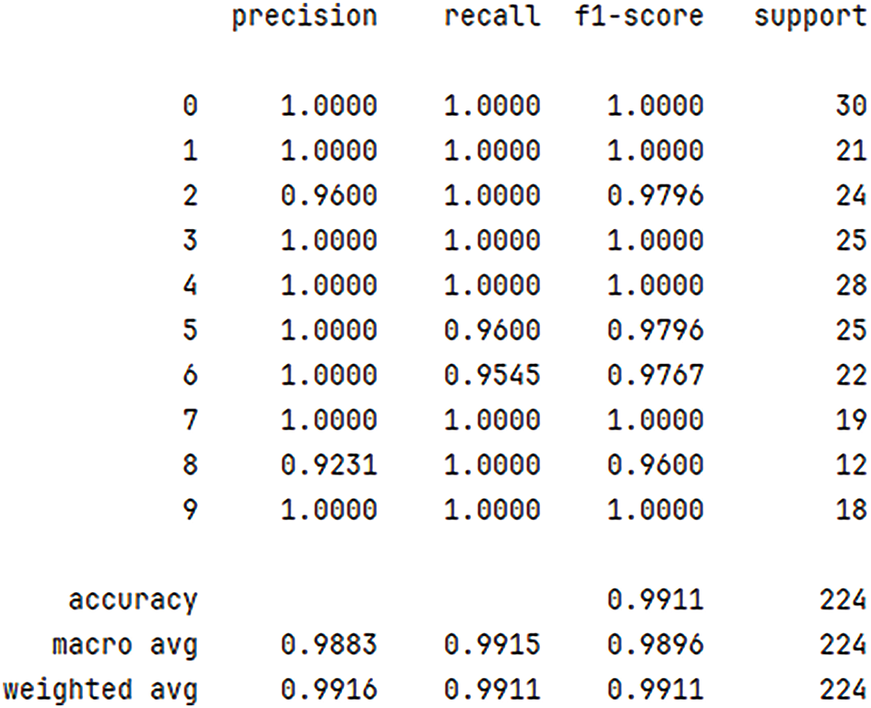
Figure 8: Performance evaluation

Figure 9: Confusion matrix

Figure 10: Initial data visualization

Figure 11: Model training visualization

To further illustrate the performance of the model in this paper, it is compared with the classical CNN, LSTM, BILSTM, CNN-BILSTM, and WDCNN-BILSTM, five models. The hyperparameters of WDCNN and BILSM are set to the same hyperparameters as in the models in this paper, and the hyperparameters of CNN are the same as those of WDCNN except that the convolution kernel of the first layer and the number of convolutional layers is 3. Fig. 12 shows their confusion matrices as well as the visualization results and Fig. 13 illustrates the comparative accuracy of the five models in question, alongside the model presented in this paper.

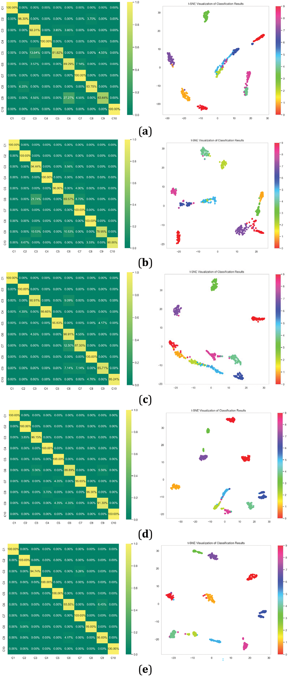
Figure 12: (a) CNN; (b) LSTM; (c) BILSTM; (d) CNN-BILSTM; (e) WDCNN-BILSTM

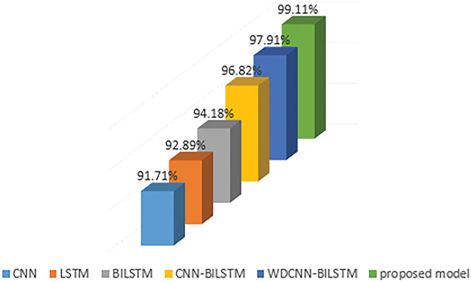
Figure 13: Comparison of model accuracy

The information in the above figure shows that the fault diagnosis model in this paper has better results and exhibits higher accuracy compared to the other classical models introduced, thus also further proving the feasibility of the model in this paper.

3.4 Noise Test

Gaussian white noise with signal-to-noise ratios (SNR) of −5, −2, 2, and 5 was added to the CWRU data set, respectively. The model proposed in this paper was then employed to analyze the data with added noise, and the confusion matrix results were presented in Fig. 14.

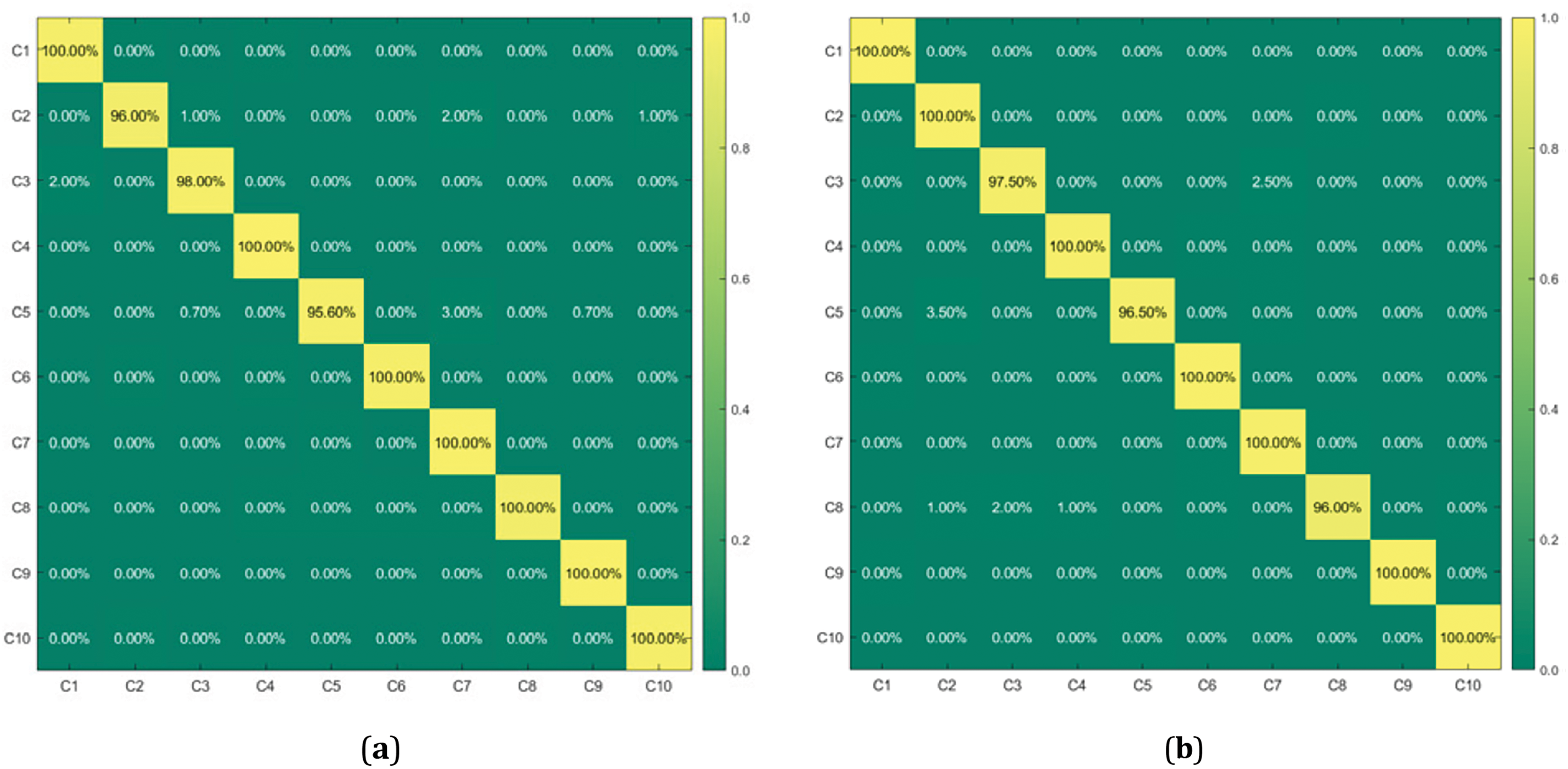
Figure 14: (a) SNR = −5; (b) SNR = −2; (c) SNR = 2; (d) SNR = 5

As demonstrated by the confusion matrix, the proposed model demonstrates an accuracy of approximately 99%, even when the SNR of Gaussian white noise is set to −5, thereby substantiating the model’s viability.

4  Experimental Verifications

The feasibility of the model in this paper was demonstrated by using the bearing dataset from Case Western Reserve University, USA. The diagnostic model in this paper is now further validated by using the data measured by the equipment provided by Changchun University’s mechanical laboratory.

4.1 Experimental Data

The equipment used in the experiment is shown in Fig. 15, the bearing model used is a 30,205 tapered rollers bearing, and EDM is used to set up the single-point failure of the bearing, which contains four kinds of states: normal, inner ring failure, outer ring failure, and rolling body failure. The rotational speed of the motor of the experimental equipment is set to 3000 r/min, the radial load is added, the load is set to 2000 N, and the sampling frequency is 20 KHz. The data set is divided according to the same principle as above, and still, the sample length of each data set is 1024, the overlap rate is 0.5, and the samples are divided according to the ratio of 0.7, 0.2, 0.1. Therefore, 233 samples are set for each fault category, and the data set contains a total of 932 samples. Each sample contains 1024 data points. The specific data situation is displayed in Table 4.

Figure 15: Diagram of experimental equipment

Meanwhile, to demonstrate the efficacy of the model in a challenging noise environment, this study introduces varying levels of Gaussian white noise into the measured vibration signals and changes the strength of the Gaussian white noise by changing the value of the signal-to-noise ratio. In this paper, we add SNR = −5, −2, 2, 5, 4 different noise signals, respectively, to validate the model in the presence of noise. Fig. 16 shows the original signals for the 4 states of the bearing (top side), and the signals after adding a SNR of −5 (bottom side).

Figure 16: (a) Normal state; (b) Inner ring fault state; (c) Outer ring fault state; (d) Rolling element fault state

4.2 Result Analysis

The noise signal is generated by different signal-to-noise ratios and substituted into the model of this paper to compare with other models and the results of the comparative analysis are presented in Table 5. Where the Raw signal denotes the original signal without adding any signal-to-noise ratio.

As illustrated in the table, the decline in accuracy of this paper’s model is less pronounced than that of the other models when the SNR is reduced, with the strongest effect on the CNN model. Especially at SNR = −5, the other models show a large decrease, which is more than 3%. However, the model in this paper only decreases by about 1.14%, which further proves that the model in this paper has good noise immunity and high robustness.

To clearly show the performance of the model, the accuracy rate, recall rate, F1 score, and accuracy rate are also used to evaluate the model, and the results are shown in Fig. 17. Meanwhile, Figs. 18–20 show the confusion matrix diagram, visualization of initial data, and classification of data after model training.

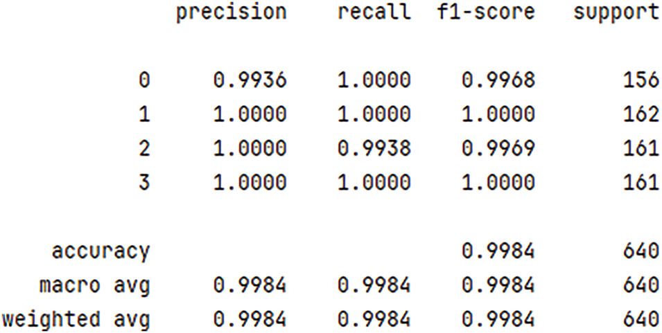
Figure 17: Performance evaluation

Figure 18: Confusion matrix

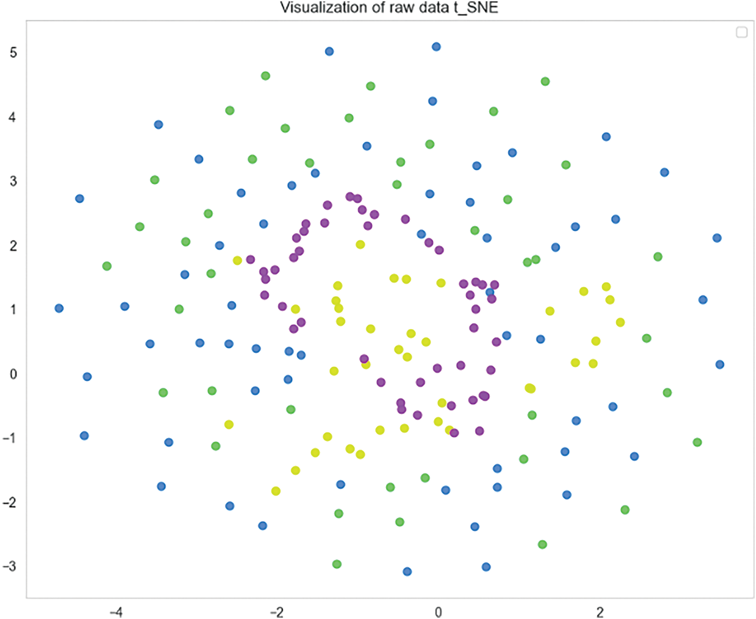
Figure 19: Initial data visualization

Figure 20: Model training visualization

Fig. 21 illustrates the confusion matrix and the classification visualization results of this paper’s model, which has been modified to include varying signal-to-noise ratios in addition to the original signal. The accuracy comparison graph is shown in Fig. 22.

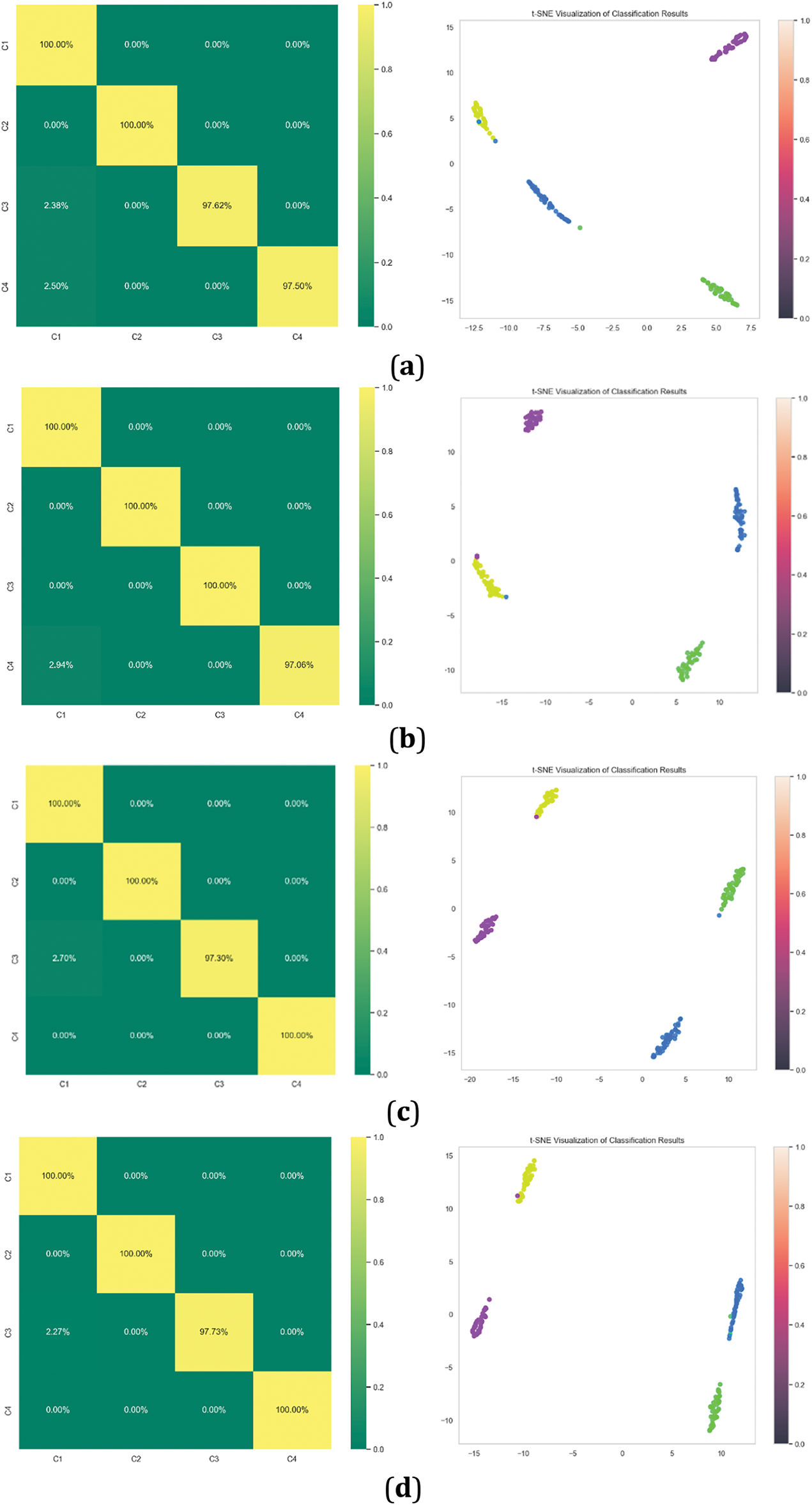
Figure 21: (a) Signal when SNR = −5; (b) Signal when SNR = −2; (c) Signal when SNR = 2; (d) Signal when SNR = 5

Figure 22: Comparison of accuracy rates under different noises

Although the model in this paper shows good performance, it is undeniable that there are still potential limitations. For deep learning models, problems such as model overfitting, hyperparameter setting, and deployment in dynamic industrial environments are inevitable. These problems can be avoided as much as possible by data enhancement, robustness experiments, and other methods. Therefore, more bearing failure datasets covering different working conditions are needed in the future to verify the universality and generalization ability of the model.

5  Conclusion

To address the challenges posed by the low accuracy and instability of the model resulting from noise in rolling bearing fault diagnosis, a network model based on cross-attention fusion WDCNN and BILSTM was proposed in this study. The efficacy of this model was substantiated through experimental verification. Initially, to mitigate the impact of noise on the diagnostic process, the original signal is decomposed into multiple modes by using VMD, and the modes containing more fault information are reconstructed by envelope entropy and kurtosis screening, which significantly improves the quality of the input data. Concerning the model architecture, spatial features are extracted by WDCNN, temporal features are extracted by BILSTM, and dynamic fusion of features is realized by cross-attention mechanism, thus enabling more comprehensive capture of fault mode information in signals.

The experimental results show that:

1.    The accuracy of diagnosis on the open-source data set is 99.11%, which is a substantial improvement on the traditional method, and serves to fully verify the effectiveness of the model.

2.    Following the incorporation of Gaussian white noise with varying signal-to-noise ratios, the model exhibits a high degree of diagnostic accuracy, thereby demonstrating its capacity for anti-noise properties and robustness.

3.    In comparison with conventional diagnostic models, this model exhibits clear advantages in terms of accuracy, robustness, and convergence speed.

The findings of this study demonstrate that the fusion model of WDCNN and BILSTM, founded on cross-attention, is capable of enhancing the precision of rolling bearing fault identification, whilst exhibiting notable resilience in noisy environments. This provides a theoretical basis and practical reference for real-time fault monitoring and diagnosis in industrial scenarios. Future work will focus on the lightweight design of the model to accommodate real-time deployment requirements in dynamic industrial environments.

Acknowledgement: The authors wish to express their appreciation to the reviewers for their helpful suggestions which greatly improved the presentation of this paper.

Funding Statement: This research was funded by the Jilin Provincial Department of Science and Technology, grant number 20230101208JC.

Author Contributions: The authors confirm their contribution to the paper as follows: Study conception and design: Yingyong Zou, Xingkui Zhang and Tao Liu; data collection: Yu Zhang and Long Li; analysis and interpretation of results: Yingyong Zou, Xingkui Zhang and Wenzhuo Zhao; draft manuscript preparation: Yingyong Zou and Xingkui Zhang. All authors reviewed the results and approved the final version of the manuscript.

Availability of Data and Materials: Data is available on request from the authors. The data that support the findings of this study are available from the corresponding author upon reasonable request.

Ethics Approval: Not applicable.

Conflicts of Interest: The authors declare no conflicts of interest to report regarding the present study.

References

1. Rai A, Upadhyay SH. A review on signal processing techniques utilized in the fault diagnosis of rolling element bearings. Tribol Int. 2016;96(4):289–306. doi:10.1016/j.triboint.2015.12.037. [Google Scholar] [CrossRef]

2. El-Thalji I, Jantunen E. A summary of fault modelling and predictive health monitoring of rolling element bearings. Mech Syst Signal Process. 2015;60(7):252–72. doi:10.1016/j.ymssp.2015.02.008. [Google Scholar] [CrossRef]

3. Yi H, Hou L, Gao P, Chen Y. Nonlinear resonance characteristics of a dual-rotor system with a local defect on the inner ring of the inter-shaft bearing. Chin J Aeronaut. 2021;34(12):110–24. doi:10.1016/j.cja.2020.11.014. [Google Scholar] [CrossRef]

4. Tao H, Wang P, Chen Y, Stojanovic V, Yang H. An unsupervised fault diagnosis method for rolling bearing using STFT and generative neural networks. J Frankl Inst. 2020;357(11):7286–307. doi:10.1016/j.jfranklin.2020.04.024. [Google Scholar] [CrossRef]

5. Maqsood A, Oslebo D, Corzine K, Parsa L, Ma Y. STFT cluster analysis for DC pulsed load monitoring and fault detection on naval shipboard power systems. IEEE Trans Transp Electrif. 2020;6(2):821–31. doi:10.1109/TTE.2020.2981880. [Google Scholar] [CrossRef]

6. Li Y, Ding K, He G, Jiao X. Non-stationary vibration feature extraction method based on sparse decomposition and order tracking for gearbox fault diagnosis. Measurement. 2018;124:453–69. doi:10.1016/j.measurement.2018.04.063. [Google Scholar] [CrossRef]

7. Wu C, Jiang P, Ding C, Feng F, Chen T. Intelligent fault diagnosis of rotating machinery based on one-dimensional convolutional neural network. Comput Ind. 2019;108(1):53–61. doi:10.1016/j.compind.2018.12.001. [Google Scholar] [CrossRef]

8. Wan L, Chen Y, Li H, Li C. Rolling-element bearing fault diagnosis using improved LeNet-5 network. Sensors. 2020;20(6):1693. doi:10.3390/s20061693. [Google Scholar] [PubMed] [CrossRef]

9. Dragomiretskiy K, Zosso D. Variational mode decomposition. IEEE Trans Signal Process. 2014;62(3):531–44. doi:10.1109/TSP.2013.2288675. [Google Scholar] [CrossRef]

10. Chen X, Yang Y, Cui Z, Shen J. Vibration fault diagnosis of wind turbines based on variational mode decomposition and energy entropy. Energy. 2019;174:1100–9. doi:10.1016/j.energy.2019.03.057. [Google Scholar] [CrossRef]

11. Jiang X, Wang J, Shen C, Shi J, Huang W, Zhu Z, et al. An adaptive and efficient variational mode decomposition and its application for bearing fault diagnosis. Struct Health Monit. 2021;20(5):2708–25. doi:10.1177/1475921720970856. [Google Scholar] [CrossRef]

12. Li F, Li R, Tian L, Chen L, Liu J. Data-driven time-frequency analysis method based on variational mode decomposition and its application to gear fault diagnosis in variable working conditions. Mech Syst Signal Process. 2019;116(1):462–79. doi:10.1016/j.ymssp.2018.06.055. [Google Scholar] [CrossRef]

13. Li Y, Cheng G, Liu C, Chen X. Study on planetary gear fault diagnosis based on variational mode decomposition and deep neural networks. Measurement. 2018;130(1):94–104. doi:10.1016/j.measurement.2018.08.002. [Google Scholar] [CrossRef]

14. Liu L, Chen L, Wang Z, Liu D. Early fault detection of planetary gearbox based on acoustic emission and improved variational mode decomposition. IEEE Sens J. 2021;21(2):1735–45. doi:10.1109/JSEN.2020.3015884. [Google Scholar] [CrossRef]

15. Wang B, Lei Y, Li N, Wang W. Multiscale convolutional attention network for predicting remaining useful life of machinery. IEEE Trans Ind Electron. 2021;68(8):7496–504. doi:10.1109/TIE.2020.3003649. [Google Scholar] [CrossRef]

16. Yang B, Liu R, Zio E. Remaining useful life prediction based on a double-convolutional neural network architecture. IEEE Trans Ind Electron. 2019;66(12):9521–30. doi:10.1109/TIE.2019.2924605. [Google Scholar] [CrossRef]

17. Li Q, Tang B, Deng L, Xiong P, Zhao M. Cross-attribute adaptation networks: distilling transferable features from multiple sampling-frequency source domains for fault diagnosis of wind turbine gearboxes. Measurement. 2022;200(2):111570. doi:10.1016/j.measurement.2022.111570. [Google Scholar] [CrossRef]

18. Alzubaidi L, Zhang J, Humaidi AJ, Al-Dujaili A, Duan Y, Al-Shamma O, et al. Review of deep learning: concepts, CNN architectures, challenges, applications, future directions. J Big Data. 2021;8(1):53. doi:10.1186/s40537-021-00444-8. [Google Scholar] [PubMed] [CrossRef]

19. Li X, Zhang W, Ding Q. Deep learning-based remaining useful life estimation of bearings using multi-scale feature extraction. Reliab Eng Syst Saf. 2019;182(7):208–18. doi:10.1016/j.ress.2018.11.011. [Google Scholar] [CrossRef]

20. Jin G, Zhu T, Akram MW, Jin Y, Zhu C. An adaptive anti-noise neural network for bearing fault diagnosis under noise and varying load conditions. IEEE Access. 2020;8:74793–807. doi:10.1109/ACCESS.2020.2989371. [Google Scholar] [CrossRef]

21. Zhang W, Peng G, Li C, Chen Y, Zhang Z. A new deep learning model for fault diagnosis with good anti-noise and domain adaptation ability on raw vibration signals. Sensors. 2017;17(2):425. doi:10.3390/s17020425. [Google Scholar] [PubMed] [CrossRef]

22. Sabir R, Rosato D, Hartmann S, Guehmann C. LSTM based bearing fault diagnosis of electrical machines using motor current signal. In: 2019 18th IEEE International Conference on Machine Learning and Applications (ICMLA); 2019 Dec 16–19; Boca Raton, FL, USA. p. 613–18. doi:10.1109/icmla.2019.00113. [Google Scholar] [CrossRef]

23. Qiu D, Liu Z, Zhou Y, Shi J. Modified bi-directional LSTM neural networks for rolling bearing fault diagnosis. In: ICC 2019—2019 IEEE International Conference on Communications (ICC); 2019 May 20–24; Shanghai, China. p. 1–6. doi:10.1109/icc.2019.8761383. [Google Scholar] [CrossRef]

24. Kumar P, Raouf I, Song J, Prince, Kim HS. Multi-size wide kernel convolutional neural network for bearing fault diagnosis. Adv Eng Softw. 2024;198:103799. doi:10.1016/j.advengsoft.2024.103799. [Google Scholar] [CrossRef]

25. Wu C, Zheng S. Fault diagnosis method of rolling bearing based on MSCNN-LSTM. Comput Mater Contin. 2024;79(3):4395–411. doi:10.32604/cmc.2024.049665. [Google Scholar] [CrossRef]

26. Xu Z, Li C, Yang Y. Fault diagnosis of rolling bearings using an Improved Multi-Scale Convolutional Neural Network with Feature Attention mechanism. ISA Trans. 2021;110(3):379–93. doi:10.1016/j.isatra.2020.10.054. [Google Scholar] [PubMed] [CrossRef]

27. Wang D, Li Y, Jia L, Song Y, Wen T. Attention-based bilinear feature fusion method for bearing fault diagnosis. IEEE/ASME Trans Mechatron. 2023;28(3):1695–705. doi:10.1109/TMECH.2022.3223358. [Google Scholar] [CrossRef]

28. Zhang Q, Wei X, Wang Y, Hou C. Convolutional neural network with attention mechanism and visual vibration signal analysis for bearing fault diagnosis. Sensors. 2024;24(6):1831. doi:10.3390/s24061831. [Google Scholar] [PubMed] [CrossRef]

29. Gao Z, Wang Y, Li X, Yao J. Twins transformer: rolling bearing fault diagnosis based on cross-attention fusion of time and frequency domain features. Meas Sci Technol. 2024;35(9):096113. doi:10.1088/1361-6501/ad53f1. [Google Scholar] [CrossRef]

30. Brocki Ł., Marasek K. Deep belief neural networks and bidirectional long-short term memory hybrid for speech recognition. Arch Acoust. 2015;40(2):191–5. doi:10.1515/aoa-2015-0021. [Google Scholar] [CrossRef]

31. Zhu X, Sobihani P, Guo H. Long short-term memory over recursive structures. In: International Conference on Machine Learning; 2015 Jul 6–11; Lille, France. p. 1604–12. [Google Scholar]

32. Wang H, Liu Z, Peng D, Cheng Z. Attention-guided joint learning CNN with noise robustness for bearing fault diagnosis and vibration signal denoising. ISA Trans. 2022;128(2):470–84. doi:10.1016/j.isatra.2021.11.028. [Google Scholar] [PubMed] [CrossRef]

33. Dibaj A, Ettefagh MM, Hassannejad R, Ehghaghi MB. A hybrid fine-tuned VMD and CNN scheme for untrained compound fault diagnosis of rotating machinery with unequal-severity faults. Expert Syst Appl. 2021;167:114094. doi:10.1016/j.eswa.2020.114094. [Google Scholar] [CrossRef]