Using Outlier Detection to Identify Grey-Sheep Users in Recommender Systems: A Comparative Study

1  Introduction

Recommender systems (RSs) are tools that use data and algorithms to predict and suggest items that match a user’s preferences or needs. These algorithms are typically divided into three main categories: content-based methods, collaborative filtering (CF), and hybrid approaches. CF algorithms, such as the neighborhood-based CF [1], matrix factorization [2], and neural collaborative filtering [3], have become one of the most widely adopted techniques due to its simplicity, flexibility in design, and ability to produce effective recommendations.

There are three major challenges in CF: rating sparsity [4], cold-start problems [5], and the presence of grey-sheep (GS) users [6–9]. GS users are individuals with unique preferences that deviate significantly from the majority, which can reduce the effectiveness of CF methods. While various approaches have been proposed to address sparsity and cold-start challenges, solutions for handling GS users remain underexplored. Prior studies [6,7] consistently categorize GS users as outliers within user groups. Researchers have generally recommended separating GS users from mainstream users and employing alternative algorithms, such as content-based methods, to provide recommendations for them [6,10,11]. Although outlier detection techniques are well-studied in data mining and machine learning [12], it is surprising that only limited outlier detection approaches were examined for identifying GS users in recommender systems. This paper seeks to address this gap by conducting an empirical analysis by using a set of comprehensive outlier detection methods for identifying GS users in recommendation systems.

In this paper, we first propose three methods for representing users, to prepare the data for outlier detection. In addition, we deliver an empirical analysis of outlier detection methods for detecting GS users and identify the approaches that can surpass the effectiveness of methodologies in prior studies. Furthermore, we provide deeper insights into the interplay between user representations and outlier detection methodologies.

2  Related Work

In this section, we introduce and discuss relevant research to our studies in this paper, including collaborative filtering, GS users, and the development of outlier detection.

2.1 Collaborative Filtering

CF is a fundamental method in recommender systems that leverages the collective preferences and actions of users to generate personalized recommendations. Traditional CF methods are often based on neighborhood-based techniques, such as user-based k-nearest neighbor (UserKNN) CF [13] and item-based KNN CF [14]. For instance, UserKNN operates on the premise that users with similar past preferences or interactions are likely to rate items in a comparable manner. The rating prediction function in UserKNN is expressed in Eq. (1), where a represents the target user, i denotes the target item, and Na is the set of k users most similar to a. The neighbor u’s rating for item i is indicated by ru,i, while the sim function (e.g., Pearson correlation, cosine similarity, or other metrics) measures similarity between users based on co-rated items. The algorithm ultimately computes Pa,i, which is the predicted rating that user a is likely to assign to the item i.

Pa,i=r¯a+∑u∈Na(ru,i−r¯u)×sim(a,u)∑u∈Nasim(a,u)(1)

The emergence of latent-factor models has positioned matrix factorization [15] as a prominent approach in CF-based RSs, primarily for its effectiveness in mitigating rating sparsity issues. In this method, users and items are represented as vectors corresponding to latent factors, which encapsulate the underlying characteristics influencing user preferences. For instance, in the context of movies, these factors might include genres, actors, or directors. A user vector thus reflects the relative importance a particular user assigns to these latent attributes. More recently, advancements such as neural matrix factorization and neural collaborative filtering models [16], or CF based on graph neural networks [17,18], have been introduced, leveraging the flexibility of generalized matrix factorization within neural network architectures to further enhance recommendation performance.

2.2 Grey-Sheep Users

The issue of cold start is a well-known challenge in CF approaches. The cold-start users refer to the new users in the system, where we have no preference data (such as ratings) rated to these users. Grey-sheep users refer to the set of users who have unusual tastes, and we do have user preferences related to these users. Despite the availability of various solutions aimed at addressing the sparsity issue and cold-start problems in CF, the challenge posed by GS users remains an area of ongoing research. Early studies primarily focused on defining GS users, initially considering them individuals with atypical preferences who neither align with nor contradict the preferences of other users [10,19]. Later, McCrae et al. categorized users in RSs into three distinct types [19]. The majority of users are classified as White Sheep, characterized by strong rating correlations with many other users. Conversely, Black Sheep users typically exhibit few or no correlations with other users, which can be tolerated in the context of rating sparsity. The real challenge, however, lies in identifying GS users, who have unique preferences or unconventional tastes, resulting in low correlations with most other users and leading to atypical recommendations for their peers. As a result, GS users are often described as “a small number of individuals who would not benefit from pure collaborative filtering systems because their opinions do not consistently agree or disagree with any group of people” [20]. It is widely accepted that GS users should be segregated from regular user groups, with alternative recommendation methods, such as content-based approaches, applied to these users [6,10,11]. Consequently, the primary research challenge remains the identification of GS users within recommender systems.

In addition, various clustering techniques [10,21,22] have been developed to identify GS users. Ghazanfar et al. [10,21] were among the first to attempt distinguishing GS users from regular users and apply content-based recommendation algorithms to enhance the recommendations for these users compared to those generated by UserKNN. Their approach was based on the assumption that GS users might be located at the boundaries of user clusters. To address this, they modified the KMeans++ clustering algorithm and introduced a new centroid selection strategy to identify users on the edges of clusters. However, their method has notable limitations, such as the difficulty in determining the optimal number of clusters and the high computational cost associated with the clustering process. Additionally, the approach is sensitive to variations in initial conditions and other parameters. Their experiments demonstrated that content-based recommendation methods could improve the recommendation performance for GS users. In contrast, Gras et al. [6] focused on outlier detection by analyzing the distribution of user ratings and factoring in the imprecision of ratings, such as prediction errors. While rating prediction errors can indicate whether a user might be a GS user, this method is not ideal for precise GS user identification, as significant prediction errors can arise from factors unrelated to GS users.

Based on the classifications of White, Black, and GS users, we subsequently proposed representing each user through the distribution statistics of user-user similarities [7,23] and applied the local outlier factor (LOF) method [24] to assist in the identification of GS users. A key aspect of our approach was the development of a validation technique for the identified GS users. Specifically, we hypothesized that the prediction errors for these GS users, when using the UserKNN algorithm, should be notably higher compared to the errors observed for non-GS users (i.e., regular users who are not classified as GS users).

2.3 Outlier Detection

Outlier detection [12] is a popular category in data mining and machine learning, and it has been successfully applied in different domains to identify outliers or anomalies. Surprisingly, no studies have directly compared these methods for identifying GS users in recommender systems. Existing literature either introduces novel, tailored approaches [10,21] or applies a single, limited outlier detection method (such as LOF) [7,23] to detect GS users within recommendation systems.

Anomaly detection involves techniques designed to identify patterns or observations that significantly deviate from the norm within a given dataset [25,26]. The primary objective of outlier detection is to scan large datasets and isolate observations with unique or unusual characteristics, enabling analysts and systems to focus on these exceptional cases. Outlier detection methods can be generally divided into three broad categories: supervised [27], unsupervised [28], and semi-supervised [29] techniques. In 2019, the PyOD toolbox [30] was introduced as an open-source platform for scalable outlier detection, incorporating a range of state-of-the-art methods. These methods can be grouped into four distinct categories:

•   Proximity-based methods are grounded in estimating neighborhoods (e.g., the KNN method [31]) or the density of data clusters (e.g., the LOF technique [24]).

•   Linear models focus on defining boundaries or representations that characterize normal data patterns, such as the One-Class SVM [32] and principal component analysis (PCA) [33].

•   Neural network-based techniques, such as AutoEncoder variants [34], use advanced architectures to reconstruct input data and identify outliers by evaluating discrepancies between the original and reconstructed data.

•   Ensemble approaches leverage the combined power of multiple base models to improve the robustness of outlier detection. For instance, the Isolation Forest [35] employs an ensemble of isolation trees to efficiently detect outliers.

It is important to highlight that the majority of outlier detection methods in PyOD are designed to work with unlabeled data. These techniques generate outlier scores, which can be used to rank data points and identify the top-ranked ones as outliers. In the context of identifying GS users, where no labels are available, we apply these methods in an unsupervised manner.

3  Data Sets, User Representations and Workflow

3.1 Data Sets

We aim to leverage the PyOD library to conduct an empirical comparison of state-of-the-art outlier detection methods for identifying GS users in recommender systems. To this end, we selected two datasets for our benchmark experiments. The first dataset is the widely used MovieLens data1, which contains 100,000 ratings provided by 943 users across 1682 movies, resulting in a rating sparsity of 93.7%. The second dataset is the Yahoo!Movie data2, where we focused on a subset of the data consisting of ratings from users who provided at least 20 ratings. This subset includes 450,067 ratings from 811 users across 3066 movies, with a rating sparsity of 98.2%. For both datasets, we only considered ratings from users who have rated at least 20 items.

3.2 User Representations

For outlier detection, we need to figure out ways to represent users (i.e., a row vector or a data point in the data set). In this paper, we propose and compare three types of user representations–user-user similarity distributions, user latent-factor vectors, and enhanced user-user dissimilarity distributions.

3.2.1 User-User Similarity Distributions

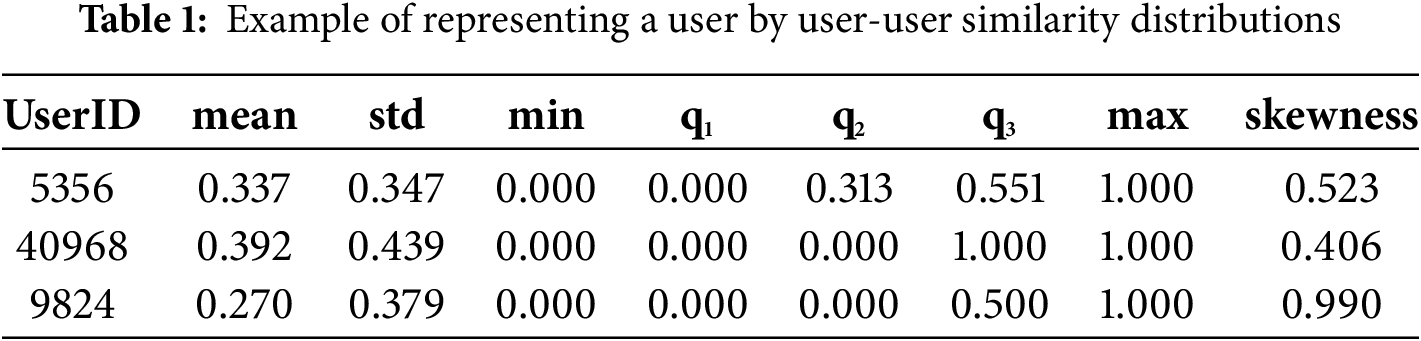
A user can be represented through the distribution statistics of user-user similarity measures, a method proven to outperform clustering-based identification techniques [7]. Specifically, the optimal similarity measure, i.e., the mean squared difference in our experiments for the two datasets, is employed to compute pairwise user-user similarities. For each user, their similarity with all other users is calculated. The user is then represented as a vector comprising distribution statistics of these similarities, including metrics such as minimum, maximum, mean, first quartile (q1), median (q2), third quartile (q3), standard deviation (std), and skewness. One example can be shown by Table 1.

3.2.2 User Latent-Factor Vectors

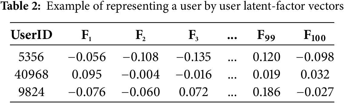
Users can also be represented using latent vectors derived from matrix factorization, where each latent factor corresponds to an underlying reason for a user’s preferences. The values in these vectors indicate the significance of these factors for a specific user. In our experiments, the optimal number of latent factors for both datasets was determined to be 100. Consequently, each user was represented by a latent vector with 100 dimensions. Notably, this form of representation has not been applied to existing methods for identifying GS users. An illustrative example is provided in Table 2, where the F columns denote the latent factors.

3.2.3 Enhanced User-User Dissimilarity Distributions

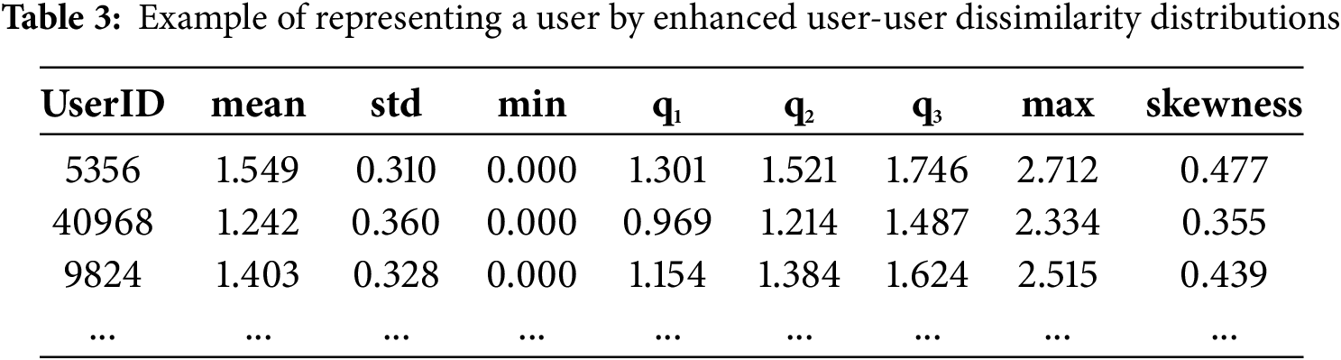
The user-user similarity distributions in Section 3.2.1 were generated from users’ ratings on the items. However, these similarities and similarity distributions may not be reliable if ratings are sparse. By contrast, we can represent users by the latent-factor vectors from matrix factorization first and then calculate user-user similarities from these user latent-factor vectors. In our experiments, we tried different similarity and dissimilarity measures. Finally, we found that using the Euclidean distance between two user latent-factor vectors is the best way to represent dissimilarities since we can identify more GS users by using it. We still utilize the minimum, maximum, mean, first quartile (q1), median (q2), third quartile (q3), standard deviation (std), and skewness as the distribution statistics to represent a user. An example can be shown by Table 3.

We assume this representation from enhanced dissimilarity distribution can work better than the representation by using the traditional similarity distribution since latent-factor models can alleviate the sparsity issue and thus the derived dissimilarities could be more accurate. In Fig. 1, we plot users based on their representations by using user-user similarity distributions depicted by shown by Fig. 1a and the enhanced user-user dissimilarity distributions shown by Fig. 2a. In these plots, we utilize skewness as the y-axis, and we select max, q1, q2, and 13 as x-axes. In Fig. 1a, we can observe some straight-line patterns, e.g., several users with the maximal similarity value of 1.0. These straight lines may lead to difficulties in identifying outliers. By contrast, there are no such line patterns in the plots based on the enhanced user-user dissimilarity distributions, and it is more straightforward for us to observe outliers from Fig. 2a. Similar conclusions can also be drawn from the plots based on Yahoo!Movie data, which can be observed from Fig. 2.

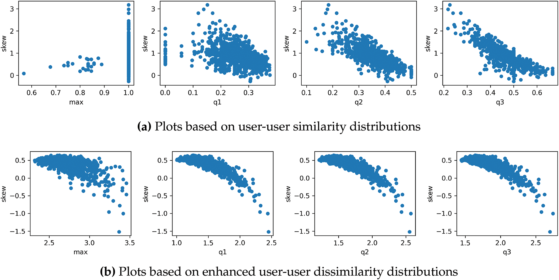
Figure 1: User plots in the MovieLens data

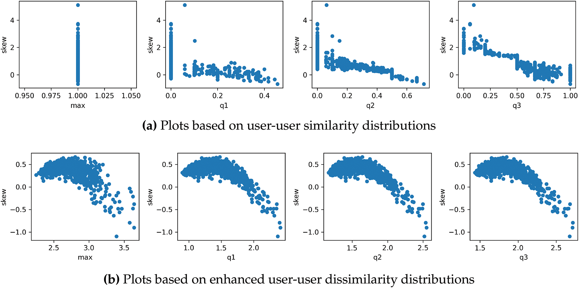
Figure 2: User plots in the Yahoo!Movies data

3.3 Workflow

Once we can represent users in our data, we move forward to run outlier detection by using the following steps. The workflow below also defined the approach for evaluations.

First of all, we applied the UserKNN and matrix factorization models to the two datasets, fine-tuning their hyperparameters to achieve the best configurations. For the UserKNN model, this involved adjusting the number of neighbors and experimenting with various similarity measures, including Pearson correlation, cosine similarity, and mean squared difference. For the matrix factorization model, a grid search approach was employed to identify the optimal values for the number of latent factors, maximum learning iterations, learning rate, and regularization parameters. We record prediction errors for each user using the optimal UserKNN model, which serves as a basis for validating the identified GS users. As highlighted in earlier studies [7,23], the presence of GS users greatly impacts the performance of UserKNN, leading to significantly higher prediction errors for these users compared to regular ones. Although matrix factorization may mitigate the impact of GS users to some extent, we rely exclusively on the prediction errors from UserKNN for validation purposes to enhance the identification process of GS users.

Furthermore, we can start running outlier detection based on different user representations. Building upon prior research that established the effectiveness of applying the LOF method to user representations based on similarity distributions, we adopt LOF as a baseline for this study. We conduct a comprehensive empirical evaluation of various outlier detection techniques available in the PyOD library to identify GS users within the two selected datasets. To validate the identified GS users, we adopt the methodology outlined in previous research [7]. Specifically, we apply the Mann-Whitney U test to conduct hypothesis testing for two independent samples at a 99% confidence level. The test is performed on the prediction errors of two groups: the identified GS users and the remaining regular users. If the test reveals a significant difference, indicating that the prediction errors from UserKNN for GS users are substantially higher than those for regular users, we classify the identified outliers as GS users. Additionally, hyper-parameters for each outlier detection method are carefully tuned to maximize the number of outliers that can be validated as GS users using the Mann-Whitney U test.

3.4 Selected Outlier Detection Methods

The outlier detection techniques used in our experiments can be listed as follows.

3.4.1 Proximity-Based Approaches

•   Local Outlier Factor (LOF) [24]: Measures the deviation in local density of data points and identifies outliers by comparing their density to that of their neighbors. In our experiments, we varied the number of neighbors from 10 to 100, increasing by 10 at each step.

•   Angle-Based Outlier Detection (ABOD) [37]: Analyzes the angles between data points to detect anomalies, with outliers characterized by distinct angular relationships. In our experiments, we varied the number of neighbors from 10 to 100, increasing by 10 at each step.

•   Cluster-Based LOF (CBLOF) [38]: Integrates clustering and density-based strategies to identify outliers within local clusters based on their LOF values. In our experiments, we varied the number of clusters from 10 to 100, increasing by 10 at each step.

•   Histogram-Based Outlier Score (HBOS) [39]: Employs histogram analysis to score and detect anomalies based on deviations from the expected distribution. In our experiments, we varied the number of bins related to histograms from 10 to 100, increasing by 10 at each step.

•   KNN-Based Methods [40]: Includes Largest KNN (LgKNN), which identifies anomalies using the largest distances in the k-nearest neighborhood, and Average KNN (AvgKNN), which leverages average distances for outlier detection. In our experiments, we varied the number of neighbors from 10 to 100, increasing by 10 at each step.

3.4.2 Linear Models

•   One-Class SVM (OCSVM) [32]: Constructs a hyperplane to model normal data, classifying instances outside this boundary as outliers. In our experiments, we varied the kernel functions, including ‘linear’, ‘poly’, ‘rbf’, and ‘sigmoid’, for parameter tuning.

•   Principal Component Analysis (PCA) [33]: Detects anomalies by examining variations in the principal components, highlighting patterns indicative of deviations. We utilized default parameters in PyOD in our experiments.

3.4.3 Neural Network-Based Methods

•   AutoEncoders (AE) [34]: Utilizes neural networks to reconstruct input data, identifying outliers through reconstruction errors. We changed the layers and number of neurons in the layers in the process of parameter tuning, and the following layers were examined, including [4,4], [8,4,4,8], [16,8,4,4,8,16], [32,16,8,4,4,8,16,32].

•   LUNAR [41]: Combines autoencoder and graph-based techniques to detect and rank anomalies by analyzing local behaviors in the feature space. In our experiments, we varied the number of neighbors from 10 to 100, increasing by 10 at each step.

3.4.4 Ensembling Approaches

•   Isolation Forest (IFOREST) [35]: Constructs an ensemble of isolation trees to effectively separate outliers from normal data. In our experiments, we varied the number of base estimators from 20 to 200, increasing by 20 at each step.

•   Local Selective Combination of Parallel Outlier Detectors (LSCP) [42]: An unsupervised ensemble approach that selects the most effective detectors within the local region of a test instance. In the PyOD library, LSCP allows us to fuse any selected outlier detection models. We selected the two best-performing outlier detection approaches above and ran the LSCP ensemble approach in our experiments.

4  Experimental Results and Findings

4.1 UserKNN and Matrix Factorization

Based on the outlined workflow, we first applied UserKNN and matrix factorization models to the two datasets. In the MovieLens dataset, matrix factorization outperformed UserKNN, achieving a mean absolute error (MAE) of 0.719 compared to the 0.732 MAE produced by UserKNN. Conversely, in the Yahoo!Movie dataset, UserKNN demonstrated a slight advantage, attaining an MAE of 0.641, marginally better than the 0.644 recorded by matrix factorization.

For parameter optimization, the mean squared difference emerged as the most effective similarity measure for UserKNN across both datasets. The optimal number of user neighbors was determined to be 70 for MovieLens and 50 for Yahoo!Movie. In the case of matrix factorization, the ideal number of latent factors was set to 100 for both datasets, with consistent learning and regularization rates of 0.01 and 0.1, respectively. The maximum number of learning iterations was optimized at 50 for MovieLens and 150 for Yahoo!Movie.

4.2 Identifying GS Users on the MovieLens Data

For outlier detection, the experimental findings for the MovieLens dataset are summarized in Tables 4 and 5. These tables present the performance outcomes of 12 distinct outlier detection techniques. Among these methods, the LOF approach, which leverages the similarity distribution as the user representation, is treated as the baseline for comparison [7].

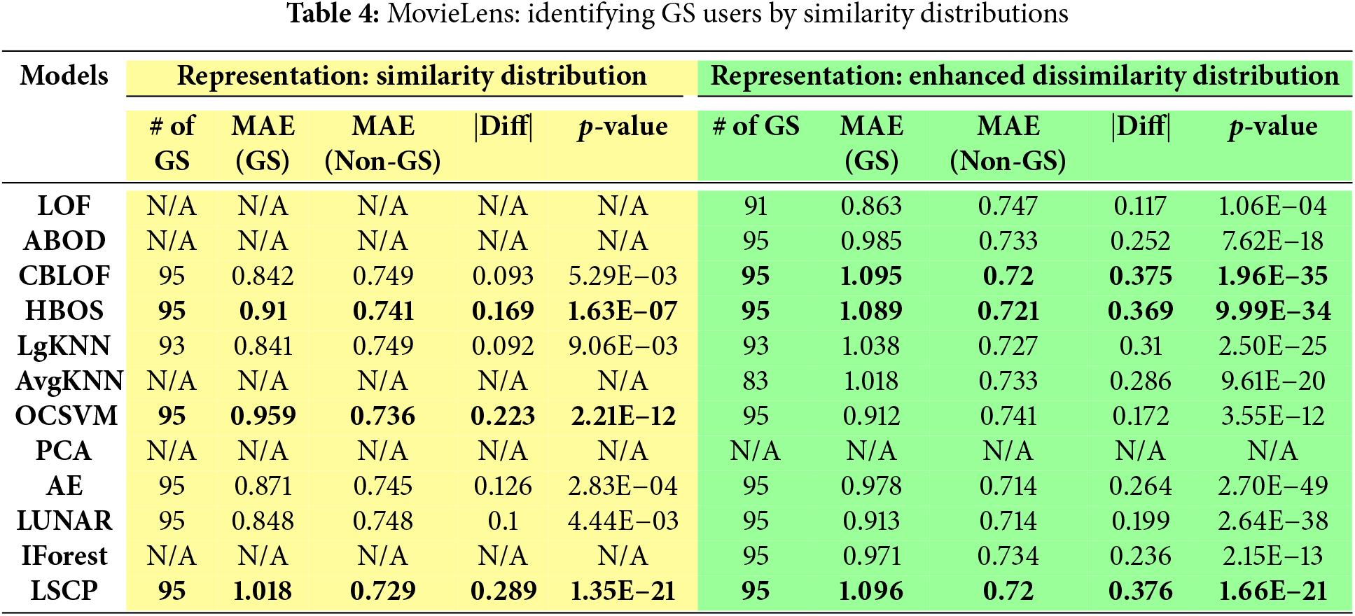
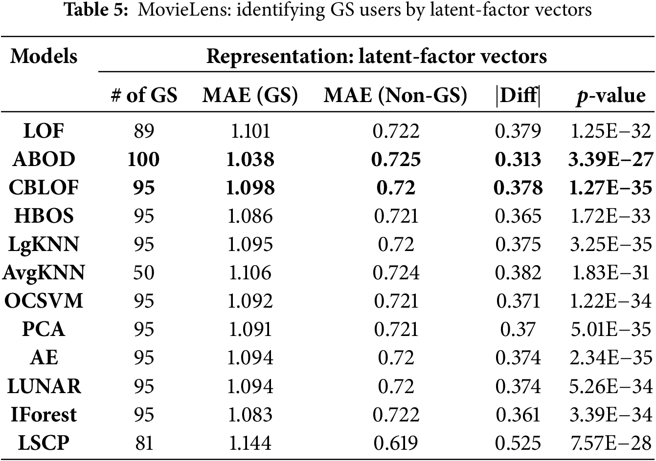
In Table 4, columns highlighted in yellow represent results obtained using similarity distribution as user representations, while green-highlighted columns correspond to results derived from the enhanced user-user dissimilarity distribution. Numbers in bold refer to the top 3 best results with largest identified GS users and larger |Diff| values. For GS user identification, the columns provide details such as the number of successfully identified GS users, the MAE values for both GS and non-GS users as calculated by UserKNN, the differences between these MAEs, and the p-values from the Mann-Whitney U test, a non-parametric test for two independent samples. If GS user identification fails, “NA” is used to denote cases where the identified outliers did not meet the 99% confidence threshold in the Mann-Whitney U test. Table 5 displays results when user latent-factor vectors are used as the representation method.

Table 4 demonstrates that up to 95 valid GS users can be identified on the MovieLens dataset when using either the similarity or dissimilarity distribution as user representations. When multiple outlier detection methods identify the same number of outliers, the column labeled “|Diff|” is used to determine the optimal method by evaluating the largest difference in MAEs. The best-performing method is identified as the one that maximizes both the number of detected GS users and the MAE difference. In this dataset, LSCP emerges as the most effective method when dissimilarity distribution is employed as the user representation. LSCP achieves its performance by integrating the top two best-performing methods (marked in bold in Table 4).

Interestingly, the baseline LOF method fails to detect GS users at a 99% confidence level in the Mann-Whitney U test when using similarity distribution as the representation. However, it successfully identifies GS users when the enhanced dissimilarity distribution is utilized. This finding highlights the superiority of using the enhanced dissimilarity distribution over the similarity distribution for representing users in this context.

Table 5 reveals that employing latent-factor vectors as user representations outperforms the use of similarity and dissimilarity distributions. Numbers in bold refer to the top two best results with larger identified GS users and larger |Diff| values. Firstly, all outlier detection methods successfully identified valid GS users, demonstrating the robustness and effectiveness of latent-factor vector representation. Secondly, the ABOD approach emerged as the most effective, identifying a higher number of valid GS users compared to other methods. Moreover, the differences in MAEs, represented by the green columns, are substantially larger than those in the yellow columns, further affirming the advantage of latent-factor vectors. In this context, the ABOD approach is the optimal model, outperforming LSCP, which did not achieve superior results despite its ensemble methodology.

4.3 Identifying GS Users on the Yahoo!Movies Data

Table 6 summarizes the results of outlier detection methods applied to Yahoo!Movie dataset, using both the enhanced dissimilarity distribution and latent-factor vectors as user representations. Numbers in bold refer to the top results with larger identified GS users and larger |Diff| values. The results obtained from the similarity distribution are excluded, as none of the outlier detection methods successfully identified valid GS users–defined as users with significantly higher MAEs than others at a 99% confidence level. However, when the confidence threshold was lowered to 95%, both the ABOD and LUNAR methods identified a subset of valid GS users. This finding reinforces the robustness and effectiveness of latent-factor vectors as user representations in GS user detection. Additionally, the results underscore the advantages of employing enhanced dissimilarity distribution for representing users. This benefit likely stems from the fact that similarities or dissimilarities derived from latent-factor vectors are more reliable compared to those based on sparse rating data.

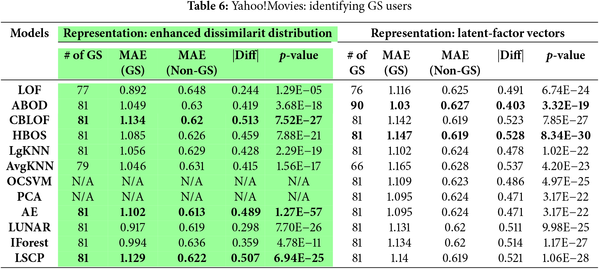
According to the results in Table 6, we can observe that ABOD is the optimal outlier detection method since it can identify the greatest number of valid GS users. The LSCP approach which combines ABOD and HBOS in this Yahoo!Movie data failed to offer further improvements or identify more valid GS users. Note that this ABOD approach also performs the best in the MovieLens data, if we use the latent-factor vectors as user representations as shown by Table 5.

4.4 Summary and Discussions

In this paper, we proposed three ways to represent users–user-user similarity distribution, enhanced user-user dissimilarity distribution, and the user latent-factor vectors, and examined the performance of a set of outlier detection based on these user representations. Our findings can be summarized as follows.

•   Based on the results obtained from the MovieLens and Yahoo!Movies datasets, we conclude that representing users through latent-factor vectors outperforms the other two representation approaches. It is not surprising that the representation method based on latent factors is better. The latent-factor models, such as matrix factorization, are well-known to alleviate the rating sparsity issues in comparison to the traditional neighborhood-based approaches. It results in better representations for users and items by using latent-factor vectors. It further leads to better results when identifying GS users in the data. By contrast, two key factors may contribute to the inability to identify valid GS users when utilizing the distribution of similarities as a representation method. First, this approach is limited by the small number of features it provides–only eight in total, including metrics such as the minimum, maximum, mean, quartiles (q1, q2, q3), standard deviation, and skewness of the similarity distribution. Second, the sparsity of data likely plays a significant role. For instance, the Yahoo!Movie dataset exhibits a rating sparsity of 98.2%. In such sparse datasets, the user-user similarities derived from co-rated items become unreliable.

•   The findings also indicate that the enhanced dissimilarity distribution serves as a superior method for user representation compared to the conventional user-user similarity distribution. It is not surprising, as the enhanced similarities or dissimilarities are derived from calculations involving user latent-factor vectors, which exhibit greater robustness in addressing challenges posed by rating sparsity.

•   There is no universal conclusion regarding the optimal outlier detection method, as its effectiveness depends on both the dataset and the type of user representation employed. In the MovieLens dataset, the ensemble approach LSCP yields the best results when using similarity or dissimilarity distributions as representations. Conversely, in the Yahoo!Movies dataset, CBLOF proves to be the most effective method when the enhanced dissimilarity distribution is used for representation. For user representations based on latent-factor vectors, ABOD consistently emerges as the most effective approach across both datasets. Unlike distance-based methods (e.g., KNN, LOF), ABOD considers the distribution of angles formed between a point and all other points, rather than just distance-based density estimates. This allows it to identify outliers more effectively in datasets where density varies significantly.

5  Conclusions and Future Work

This study introduces three distinct approaches for representing users in recommender systems: (1) the distribution statistics of user-user similarities calculated using UserKNN, (2) the enhanced user-user dissimilarity distribution, and (3) latent-factor vectors generated through matrix factorization. We conducted an empirical evaluation of cutting-edge outlier detection methods to identify genuine GS users effectively. Our findings confirm that representing users with latent-factor vectors is the most effective approach for identifying GS users, though the optimal outlier detection method varies across datasets and depends on the chosen representation technique. In future research, we plan to expand our investigation beyond movie datasets, exploring domains outside of the movie industry. Additionally, we intend to examine the distribution of atypical preferences over items (e.g., preferences across various item categories or content features) to gain deeper insights into the behavior of identified GS users. This understanding will guide the development of more effective recommendation models tailored to these users’ unique preferences.

Acknowledgement: Not applicable.

Funding Statement: The author received no specific funding for this study.

Availability of Data and Materials: The data source has been mentioned in Section 3.1.

Ethics Approval: Not applicable.

Conflicts of Interest: The author declares no conflicts of interest to report regarding the present study.

1The MovieLens data is available from https://grouplens.org/datasets/movielens/100k/ (accessed on 27 March 2025).

2We do not have authorization to distribute this data, but it can be acquired from the data owners or authors [36].

References

1. Nikolakopoulos AN, Ning X, Desrosiers C, Karypis G. Trust your neighbors: a comprehensive survey of neighborhood-based methods for recommender systems. In: Ricci F, Rokach L, Shapira B, editors. Recommender systems handbook. New York, NY, USA: Springer; 2021. p. 39–89. [Google Scholar]

2. Isinkaye FO. Matrix factorization in recommender systems: algorithms, applications, and peculiar challenges. IETE J Res. 2023;69(9):6087–100. doi:10.1080/03772063.2021.1997357. [Google Scholar] [CrossRef]

3. Rendle S, Krichene W, Zhang L, Anderson J. Neural collaborative filtering vs. matrix factorization revisited. In: Proceedings of the 14th ACM Conference on Recommender Systems; New York, NY, USA: ACM; 2020. p. 240–8. [Google Scholar]

4. Idrissi N, Zellou A. A systematic literature review of sparsity issues in recommender systems. Soc Netw Anal Min. 2020;10(1):15. doi:10.1007/s13278-020-0626-2. [Google Scholar] [CrossRef]

5. Panda DK, Ray S. Approaches and algorithms to mitigate cold start problems in recommender systems: a systematic literature review. J Intell Inf Syst. 2022;59(2):341–66. doi:10.1007/s10844-022-00698-5. [Google Scholar] [CrossRef]

6. Gras B, Brun A, Boyer A. Identifying grey sheep users in collaborative filtering: a distribution-based technique. In: Proceedings of the 2016 Conference on User Modeling Adaptation and Personalization; Halifax, NS, Canada: ACM; 2016. p. 17–26. [Google Scholar]

7. Zheng Y, Agnani M, Singh M. Identifying grey sheep users by the distribution of user similarities in collaborative filtering. In: Proceedings of the 6th ACM Conference on Research in Information Technology; Rochester, NY, USA: ACM; 2017. [Google Scholar]

8. Alabdulrahman R, Viktor H. Catering for unique tastes: targeting grey-sheep users recommender systems through one-class machine learning. Expert Syst Appl. 2021;166(2):114061. doi:10.1016/j.eswa.2020.114061. [Google Scholar] [CrossRef]

9. Zheng Y. An empirical comparison of outlier detection methods for identifying grey-sheep users in recommender systems. In: International Conference on Advanced Information Networking and Applications; Kitakyushu, Japan: Springer; 2024. p. 62–73. [Google Scholar]

10. Ghazanfar M, Prugel-Bennett A. Fulfilling the needs of gray-sheep users in recommender systems, a clustering solution. In: Proceedings of the 2011 International Conference on Information Systems and Computational Intelligence; Harbin, China; 2011. p. 18–20. [Google Scholar]

11. Tennakoon A, Gamlath N, Kirindage G, Ranatunga J, Haddela P, Kaveendri D. Hybrid recommender for condensed sinhala news with grey sheep user identification. In: 2020 2nd International Conference on Advancements in Computing (ICAC); 2020; IEEE. Vol. 1, p. 228–33. doi:10.1109/ICAC51239.2020. [Google Scholar] [CrossRef]

12. Boukerche A, Zheng L, Alfandi O. Outlier detection: methods, models, and classification. ACM Comput Surv. 2020;53(3):1–37. doi:10.1145/3421763. [Google Scholar] [CrossRef]

13. Resnick P, Iacovou N, Suchak M, Bergstrom P, Riedl J. GroupLens: an open architecture for collaborative filtering of netnews. In: Proceedings of the 1994 ACM Conference on Computer Supported Cooperative Work; Chapel Hill, NC, USA: ACM; 1994. p. 175–86. [Google Scholar]

14. Sarwar B, Karypis G, Konstan J, Riedl J. Item-based collaborative filtering recommendation algorithms. In: Proceedings of the 10th International Conference on World Wide Web; Ljubljana, Slovenia; 2001. p. 285–95. [Google Scholar]

15. Koren Y, Bell R, Volinsky C. Matrix factorization techniques for recommender systems. Computer. 2009;42(8):30–7. doi:10.1109/MC.2009.263. [Google Scholar] [CrossRef]

16. He X, Liao L, Zhang H, Nie L, Hu X, Chua TS. Neural collaborative filtering. In: Proceedings of the 26th International Conference on World Wide Web; Perth, Australia; 2017. p. 173–82. [Google Scholar]

17. Elahi E, Halim Z. Graph attention-based collaborative filtering for user-specific recommender system using knowledge graph and deep neural networks. Knowl Inf Syst. 2022;64(9):2457–80. doi:10.1007/s10115-022-01709-1. [Google Scholar] [CrossRef]

18. Elahi E, Anwar S, Shah B, Halim Z, Ullah A, Rida I, et al. Knowledge graph enhanced contextualized attention-based network for responsible user-specific recommendation. ACM Trans Intell Syst Technol. 2024;15(4):1–24. doi:10.1145/3641288. [Google Scholar] [CrossRef]

19. McCrae J, Piatek A, Langley A. Collaborative filtering. 2004 [cited 2025 Mar 27]. Available from: wwwimperialvioletorg. [Google Scholar]

20. Claypool M, Gokhale A, Miranda T, Murnikov P, Netes D, Sartin M. Combining content-based and collaborative filters in an online newspaper. In: Proceedings of ACM SIGIR Workshop on Recommender Systems; Berkeley, CA, USA; 1999. Vol. 60. [Google Scholar]

21. Ghazanfar MA, Prügel-Bennett A. Leveraging clustering approaches to solve the gray-sheep users problem in recommender systems. Expert Syst Appl. 2014;41(7):3261–75. doi:10.1016/j.eswa.2013.11.010. [Google Scholar] [CrossRef]

22. Kaur B, Rani S. Identification of gray sheep using different clustering algorithms. In: Proceedings of the Second International Conference on Information Management and Machine Intelligence: ICIMMI 2020; Jaipur, India: Springer; 2020. p. 211–7. [Google Scholar]

23. Zheng Y, Agnani M, Singh M. Identification of grey sheep users by histogram intersection in recommender systems. In: Advanced Data Mining and Applications: 13th International Conference; Singapore: Springer; 2017. p. 148–61. [Google Scholar]

24. Breunig MM, Kriegel HP, Ng RT, Sander J. LOF: identifying density-based local outliers. In: ACM sigmod record. Dallas, TX, USA: ACM; 2000. Vol. 29, p. 93–104. [Google Scholar]

25. Chandola V, Banerjee A, Kumar V. Anomaly detection: a survey. ACM Comput Sur. 2009;41(3):15–58. doi:10.1145/1541880.1541882. [Google Scholar] [CrossRef]

26. Hodge V, Austin J. A survey of outlier detection methodologies. Artif Intell Rev. 2004;22(2):85–126. doi:10.1023/B:AIRE.0000045502.10941.a9. [Google Scholar] [CrossRef]

27. Aggarwal CC. Supervised outlier detection. Outlier Analysis. 2017;219–48. doi:10.1007/978-3-319-47578-3. [Google Scholar] [CrossRef]

28. Campos GO, Zimek A, Sander J, Campello RJ, Micenková B, Schubert E, et al. On the evaluation of unsupervised outlier detection: measures, datasets, and an empirical study. Data Min Knowl Discov. 2016;30(4):891–927. doi:10.1007/s10618-015-0444-8. [Google Scholar] [CrossRef]

29. Gao J, Cheng H, Tan PN. Semi-supervised outlier detection. In: Proceedings of the 2006 ACM Symposium on Applied Computing; Dijon, France; 2006. p. 635–6. [Google Scholar]

30. Zhao Y, Nasrullah Z, Li Z. PyOD: a python toolbox for scalable outlier detection. J Mach Learn Res. 2019;20(96):1–7. [Google Scholar]

31. Angiulli F, Pizzuti C. Fast outlier detection in high dimensional spaces. In: European Conference on Principles of Data Mining and Knowledge Discovery; Helsinki, Finland: Springer; 2002. p. 15–27. [Google Scholar]

32. Schölkopf B, Platt JC, Shawe-Taylor J, Smola AJ, Williamson RC. Estimating the support of a high-dimensional distribution. Neural Comput. 2001;13(7):1443–71. doi:10.1162/089976601750264965. [Google Scholar] [PubMed] [CrossRef]

33. Shyu ML, Chen SC, Sarinnapakorn K, Chang L. A novel anomaly detection scheme based on principal component classifier. In: Proceedings of the IEEE Foundations and New Directions of Data Mining Workshop; Melbourne, FL, USA: IEEE Press; 2003. p. 172–9. [Google Scholar]

34. Aggarwal CC. An introduction to outlier analysis. In: Outlier analysis. Cham: Springer; 2017. [Google Scholar]

35. Liu FT, Ting KM, Zhou ZH. Isolation forest. In: 2008 Eighth IEEE International Conference on Data Mining; Pisa, Italy: IEEE; 2008. p. 413–22. [Google Scholar]

36. Jannach D, Zanker M, Fuchs M. Leveraging multi-criteria customer feedback for satisfaction analysis and improved recommendations. Inf Technol Tour. 2014;14(2):119–49. doi:10.1007/s40558-014-0010-z. [Google Scholar] [CrossRef]

37. Kriegel HP, Schubert M, Zimek A. Angle-based outlier detection in high-dimensional data. In: Proceedings of the 14th ACM SIGKDD International Conference on Knowledge Discovery and Data Mining; Las Vegas, NV, USA; 2008. p. 444–52. [Google Scholar]

38. He Z, Xu X, Deng S. Discovering cluster-based local outliers. Pattern Recognit Lett. 2003;24(9–10):1641–50. doi:10.1016/S0167-8655(03)00003-5. [Google Scholar] [CrossRef]

39. Goldstein M, Dengel A. Histogram-based outlier score (HBOSa fast unsupervised anomaly detection algorithm. KI-2012: Poster Demo Track. 2012;1:59–63. [Google Scholar]

40. Ramaswamy S, Rastogi R, Shim K. Efficient algorithms for mining outliers from large data sets. In: Proceedings of the 2000 ACM SIGMOD International Conference on Management of Data; Dallas, TX, USA; 2000. p. 427–38. [Google Scholar]

41. Goodge A, Hooi B, Ng SK, Lunar Ng WS. Unifying local outlier detection methods via graph neural networks. Proc of the AAAI Conf Artif Intell. 2022;36(6):6737–45. doi:10.1609/aaai.v36i6.20629. [Google Scholar] [CrossRef]

42. Zhao Y, Nasrullah Z, Hryniewicki MK, Li Z. LSCP: locally selective combination in parallel outlier ensembles. In: Proceedings of the 2019 SIAM International Conference on Data Mining; Calgary, AB, Canada: SAM; 2019. p. 585–93. [Google Scholar]