Multi-Firmware Comparison Based on Evolutionary Algorithm and Trusted Base Point

1  Introduction

As embedded systems evolve toward intelligentization, firmware has transitioned from simple single-function control programs (e.g., 1980s microcontroller firmware [1]) to become a core software component in complex systems. Modern firmware, such as that used in Cisco networking devices and industrial control systems (ICS), integrates advanced features like network protocol stacks, security encryption modules, and multi-architecture compatibility (ARM/X86/RISC-V). This technological advancement has caused firmware complexity to grow exponentially, introducing new security challenges such as heterogeneous compatibility verification and the detection of hidden vulnerabilities [2,3]. To address these challenges, rigorous auditing and analysis of firmware have become essential.

In recent years, binary code similarity detection [4–7] has emerged as a versatile tool for security analysis, playing a critical role in addressing the aforementioned challenges. This technology identifies function correspondences by comparing binary executables to determine their similarity. Its applications are extensive, including malware detection [8–11], plagiarism identification [12–14], vulnerability searching [15–17], and patch analysis [18–21]. In the firmware domain, binary code comparison has been further applied to firmware comparison [22], analyzing the correlation of functions between different firmware versions. As firmware continues to evolve, this capability for comparison and analysis has become indispensable for effective firmware auditing and security analysis.

While binary code comparison techniques have advanced significantly in recent years, they predominantly address one-to-one (O2O) or one-to-many (O2M) scenarios. In O2O methods, tools like BinDiff [23] analyzes pairwise structural or semantic similarities between functions in two programs using control flow graphs (CFGs) or heuristic hashing, establishing a one-to-one correspondence. DEEPBINDIFF [24] leverages machine learning and natural language processing. It combines assembly instructions with CFG structures to generate embedding vectors for each basic block in two binary programs and then iteratively searches for matching basic blocks to achieve more precise one-to-one comparisons. And in O2M methods, Genius [25] converts control flow graphs (CFGs) into high-dimensional numerical feature vectors, uses clustering algorithms to generate a set of feature vectors (i.e., codebook), and combines Locality-Sensitive Hashing (LSH) to quickly filter out candidate functions similar to the query function from a large pool. CEBin [17] integrates embedding-based and comparison-based approaches. It first uses an embedding-based method to efficiently filter out the top K candidate functions from a large-scale function pool, and then employs a comparison-based method to perform precise matching on these candidates. Currently, the study of many-to-many (M2M) comparisons between programs is relatively rare. While some works attempt multi-program analysis, they often reduce the problem to aggregated pairwise comparisons. For example, early works like Kruegel et al. [26] applied CFG graph coloring to detect worm variants, but their dataset (less than 20 MB executables) and pairwise logic limit scalability. Hu et al. [27] employed N-gram opcode features to cluster malware, whereas Farhadi et al. [28] integrated instruction-level clones. However, both approaches simplified M2M comparisons to localized pairwise matching. Even recent innovations like JTrans [29] (transformer-based function matching) and VulHawk [30] (microcode-driven cross-architecture search) extend O2M paradigms without true M2M optimization. To the best of our knowledge, no prior work explicitly addresses M2M firmware function comparison, which requires simultaneous analysis of inter-version dependencies, cross-architecture compatibility, and evolutionary code changes across multiple firmware binaries.

This paper’s main objective is to establish function correspondences between multiple firmwares. To improve the efficacy, we should construct the correspondence between firmware functions as much as possible (called matching or comparison in this paper). To perform the multi-firmware comparison, we first model the multi-firmware matching as a multi-sequence matching problem. Then we propose a fitness function and a population generation and updating method based on trusted base points and local optimal solutions. Finally, we apply an evolutionary algorithm to find the optimal result. At the same time, we design the similarity of matching results as an evaluation metric to measure the effect of multi-firmware comparison.

We evaluate the performance of the proposed method with real-world firmwares of routers. The experiments show that the similarity of matching results between the proposed method and Bindiff is 61%, and the similarity of the matching results between our solution and the string-based method is 62.8%. The accuracy of the matching results of the proposed method is about 66.4% by manual verification through sampling.

In summary, we make the following contributions:

•   To the best of our knowledge, we are the first to propose a multi-firmware comparison method based on an evolutionary algorithm. It can be used for the function correspondence construction of multi-firmware.

•   We depict the multi-firmware comparison problem with the multi-sequence comparison model and design a fitness function for the evolutionary algorithm.

•   We propose a population generation and updating method based on trusted base points and local optimal solutions for multi-firmware comparison.

•   We implement our proposed approach and verify the feasibility of our solution on real-world firmwares. The experiments illustrate that our solution outperforms Bindiff [23] (Version 5) and the string-based method.

2  Background

This section defines the multi-firmware comparison problem and then illustrates the observation with a motivation example.

2.1 Problem Definition

Inspired by bioinformatics, where conserved regions in gene sequences are identified despite mutations, our model assumes core firmware functions retain logical consistency across versions. Evolutionary algorithms search for globally optimal alignments, avoiding local optima traps inherent in syntax-based methods. To address these challenges, we model multi-firmware comparison as a multi-sequence matching problem.

Given a sequence set S={S1,S2,…,SN},N≥2,Si=Si1Si2…Sili(1≤i≤N),Sij∈Z(1≤j≤li),0≤Sij<li, and ∀ k≠j (1≤k≤li), with Sij≠Sik,li is the length of the i-th sequence, a specific inter-sequence correlation (later called multi-sequence matching) can be defined as a matrix A=(ai,j), where, 1≤i≤N, 1≤j≤l, max(li)≤L≤σi=1Nli, and the matrix needs to satisfy the following three conditions:

•   ai,j∈Z, (−1≤ai,j≤li), where −1 denotes empty space;

•   The sequence Si is obtained by removing −1 from the i-th row of the matrix;

•   The matrix does not contain columns whose values are all −1.

For N firmwares, we define the results of the multi-firmware comparison in the above way. In this paper, li denotes the number of functions in the i-th firmware, and Sij denotes the index value of the function (indexing from 0). A is called the function matching matrix, and each column in A represents the correspondence of each specific function in different firmwares. Based on the maximum firmware length and the ratio of inserted empty spaces, we can adjust the value of L. A function matching matrix of a set of firmwares is a scheme for constructing function correspondences. Therefore, a group of firmwares can have multiple functions matching matrices. This paper aims to find the most reasonable function matching matrix.

2.2 Motivation Example

Fig. 1 shows an example of a function matching matrix corresponding to a multi-firmware comparison. The functions f1 and f6 in the three firmwares P1, P2, and P3 have index values 0,0,0 and 5,5,2, respectively. The first and last columns of a function matching matrix A1 reflect the correspondence between f1 and f6 in the three firmwares. Also, the new function fnew in gray can form a correspondence with other functions (even if this correspondence is wrong) and further form a matching matrix, as long as it satisfies the previous expressions in this section.

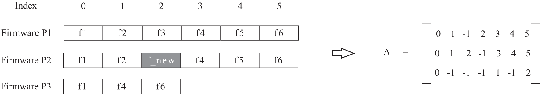
Figure 1: Example of multi-firmware sequence comparison

Since we focus on firmwares, there is an assumption that there is no randomization of function addresses. Namely, functions in firmware are generally placed in order. To facilitate the subsequent analysis, we add a condition to the above representation, if j<k, then we have Sij<Sik.

3  Evolutionary Algorithm

This paper uses the optimized evolutionary algorithm to find the best matching result of multi-firmware. Fig. 2 shows the workflow of the optimized evolutionary algorithm.

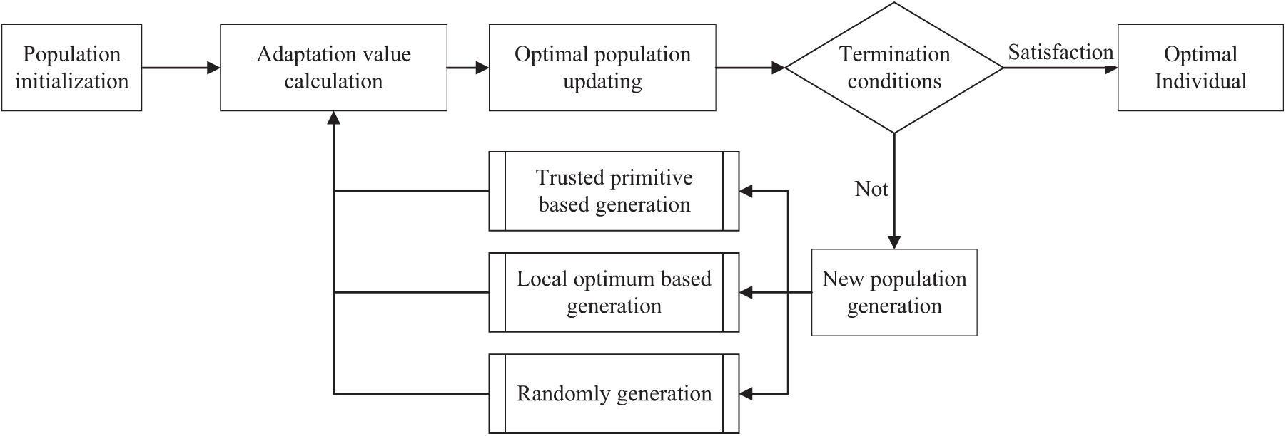
Figure 2: Workflow of optimized evolutionary algorithm

3.1 Workflow of Optimized Evolutionary Algorithm

3.1.1 Population Initialization

The initialization of the population is to provide several initial solutions (seeds). Compared with the completely random generation of function matching matrix, some relatively reliable initial solutions can be provided based on string matching and other methods for multi-firmware matching. To verify the proposed method’s effectiveness, we randomly generate the initial population.

3.1.2 Optimal Population Update

The optimal population is the optimal result accumulated over iterations. The measure of the merit of individuals in a population relies on the fitness function. Since the design of the fitness function also involves the elaboration related to the generation of new populations, we illustrate it in detail in Section 3.2. A proportional selection method and the best individual preservation strategy can update the optimal population. In the former, individuals are selected randomly according to their adaptation value, and their probability is proportional to their adaptation value. The latter is a simple selection of the individual with the highest adaptation value. For the optimal population size (i.e., the number of individuals in the optimal population, denoted as Mbest_family). In practice, it is mainly limited by the hardware environment (e.g., memory), so we do not discuss its parameters in this paper but take the maximum value allowed by the environment.

3.1.3 New Population Generation

The primary purpose of new population generation is to generate several individuals using various methods to provide a basis for updating the optimal population. The prerequisite for new population generation is to determine that there is still a chance to optimize the optimal population. If there is no chance for optimization, the optimal individuals are output directly. Generally, we determine the conditions for termination (i.e., no more updates of the optimal population) in three ways: (1) the adaptation value of the optimal individual reaches a specified size; (2) the number of population updates is more significant than a threshold; (3) the average increase in adaptation value of the optimal population after several updates is less than a threshold. In this paper, since the change of adaptation value at the beginning of the population update is small, we only rely on the number of population updates and the adaptation value of the best individual to determine the termination.

This paper adopts three methods to generate new populations: generation based on trusted base points, local optima, and random generation. The first two methods will be described in Sections 4 and 5. Random generation generates new individuals randomly according to the function matching matrix A. Random generation aims to obtain as many different matching possibilities as possible for each function, which is particularly important for population optimization, especially for generating new populations based on trusted base points.

3.2 Fitness Function

The fitness function provides a metric for evaluating individuals in a population, also referred to as the “objective function” in some studies. In this paper, the fitness function reflects the similarity of a function matching scheme between firmwares (a function matching matrix as a matching scheme). The fitness function consists of three components: feature similarity Simfea, empty position penalty Emp, and consecutive scores Con, which are shown in Eq. (1), where matrix A is the function matching matrix for multi-firmware comparison.

F(A)=Simfea(A)+Emp(A)+Con(A)(1)

3.2.1 Feature Similarity

For a multi-firmware comparison, there is a function matching matrix A=(aij), which has N rows and L columns; the number of functions li for each firmware satisfies li≤L. If Aj denotes the N-dimensional vector of the jth column in matrix A, then we have A={A1,A2,...,AL}. The feature similarity of matrix A should be calculated by Eq. (2), i.e., the feature similarity of the matching function Simfea(Aj) is calculated column by column and then averaged. Since different function matching matrices A may have a different number of columns L, we average the results to calculate the similarity. The function matching matrices with different columns can be more comparable.

Simfea(A)=Σj=1Lmax(0,Simfea(Aj))/L(2)

where max means that if the function similarity score of a single column is less than 0, the value is assigned to 0. The reason is that, for the function similarity formula in this paper, when the similarity of a single column is less than a specific value, it will not reflect whether some functions in a column have high similarity among firmwares. The difference in its similarity value is not significant for optimizing the multi-sequence matching results. Therefore, the values are truncated to reduce the impact on the cumulative total score of the function matching matrix.

The similarity calculation of the matching function for a single column should also sum the mean values after accumulation, as shown in Eq. (3).

Simfea(Aj)=Σi=1N−1Σh=i+1NSim(ai,j,ah,j)/(N∗(N−1)/2)(3)

where Sim(ai,j,ah,j) denotes the similarity of the elements at the specified position (column j) of two sequences (row i, h) in the matching matrix of a multiple sequence matching function. In biological multiple sequence matching, the similarity between residues-residues and residues-vacancies is generally calculated. There are generally substitution scoring matrices for the similarity between residues to guide the assignment, e.g., acceptable point mutation matrix (PAM), block substitution matrix (BLOSUM), etc. However, for the multi-firmware comparison in this paper, the elements of matrixA represent the indexes or empty spaces of functions, which cannot be directly applied to the replacement scoring matrix in biological multiple sequence matching. The scores of the substitution scoring matrix in bioinformatics are based on experiments and may not apply to firmware matching.

Therefore, we designs the scoring function Sim(ai,j,ah,j) applicable to firmware comparison, as shown in Eq. (4); for the convenience, a denotes the index ai,j and b denotes the index ah,j, a≥0, fi,a denotes the function with index value ai,j for the i-th firmware. The correspondence of empty space is not scored; while the correspondence of function-function is scored by the more mature binary function similarity analysis method, the value of similarity(fi,a,fh,b) is directly used as the score in this paper.

Sim(a,b)={similarity(fi,a,fh,b),a≥0⋀b≥00, a<0⋁b<0(4)

To determine the similarity(fi,a,fh,b), we should first determine the representation of the function in the firmware. We use four features to form a 4-dimensional vector to represent functions, with f=<NumI,NumB,NumSN,NumPN>, the features are the number of function instructions NumI, the number of basic blocks NumB, the number of child functions NumS_N, the number of parent functions NumP_N. We use Eq. (5) to calculate the similarity of two functions, which f1 and f2 represent the feature vectors of any two functions.

similarity(f1,f2)=Pc(f1,f2)+Ed′(f1,f2)−1(5)

Ed′(f1,f2)={11+logαEd(f1,f2),f1≠f21,f1=f2(6)

Pc denotes the Pearson Correlation Coefficient (PCC) of two vectors, and Ed denotes the Euclidean distance of two vectors. Since one of the above two indicators represents the similarity and the other represents the difference, some transformation is needed when combining them.

In the case of unequal eigenvectors, since each dimension of the eigenvector of the function is a non-negative integer, the Euclidean distance of the eigenvectors of the function must be a number greater than 1. By taking the logarithm of the Euclidean distance (with α as the base, which is recommended to take 10 in this paper) and adding 1 to the logarithm, and taking the inverse, we can ensure that the value of Ed′(f1,f2) is in the interval of (0,1); combined with the case of equal eigenvectors, Ed′(f1,f2) takes the value of (0,1]. And Pc takes the value in [0,1], thus it is known that Eq. (5) takes the value in [−1,1]. After the adjustment of Eq. (2), we can see that Eq. (2) takes the value of [0,1], and the larger the value, the higher the similarity. The four features <NumI,NumB,Num(SN),Num(PN)> are chosen to represent the functions and designed to calculate the similarity in Eq. (5), mainly to reduce the time overhead in the process of extracting information and comparison, in fact, as long as the similarity between a pair of functions can be provided, the function representation and similarity calculation can be customized. Ed′(f1,f2) can also be calculated by using the inverse of the Euclidean distance without taking the logarithm. However, this paper considers that Eq. (6) works better, which is related to the distribution of the values of the Euclidean distances of the calculated samples.

3.2.2 Empty Position Penalty

In multi-sequence matching, each sequence is not identical. Therefore, it is necessary to form a function matching matrix by inserting empty bits. Theoretically, a large number of empty bits can be inserted. In that case, any number of sequences that are not identical can form a multi-sequence matching scheme and find the corresponding multi-sequence correspondence matrix A. However, the function matching matrix formed in this scenario has no guiding meaning. Therefore, we should limit the number of empty bits. In this paper, we follow the strategy of empty penalty score, and the formula for calculating the empty penalty score of matrixA is shown in Eq. (7).

Emp(A)=Σj=1LEmp′(Aj)/LEmp′(Aj)=β∗empty_numj/N(7)

where empty_numj denotes the number of empty bits in column Aj (i.e., the number of values of −1); β denotes the maximum penalty value of single column empty bits, β<0, generally varies with the value of N. In this paper, the value of −1 is generally taken when comparing 4 sequences. In practical applications, the empty penalty and feature similarity are used jointly to evaluate the correspondence of single column functions in the function matching matrix and improve Eq. (2), as shown in Eq. (8).

Simfea(A)=Σj=1Lmax(0,Simfea′(Aj))/LSimfea′(Aj)=Emp′(Aj)+Simfea(Aj)(8)

3.2.3 Consecutive Scores

In the traditional scoring for multiple sequence matching, the empty penalty consists of two parts: one is called the starting empty penalty, which is shown as Eq. (7); and the other is called the extended empty penalty. The starting empty penalty affects the number of inserted spaces, while the extended empty penalty affects the continuity of the inserted spaces, i.e., the number of consecutive spaces. In this paper, the formula for calculating the consecutive score is designed based on the idea of extending the empty space, as shown in Eq. (9).

Con(A)=(Σj=1L−1Con′(Aj))/(L−1)Con′(Aj)=γ∗Σi=1Ncontinue(ai,j)/Ncontinue(ai,j)={1,ai,j>−1⋀ai,j+1>−1,ai,j∈Z0, ai,j>−1⋀ai,j+1<0,ai,j∈Z0, ai,j<0⋀ai,j+1>−1,ai,j∈Z1,   ai,j<0⋀ai,j+1<0,ai,j∈Z(9)

where A is a function matching matrix of N firmwares if the number of columns is L, the sequence that can calculate the consecutive score is only L−1 columns. For a column of function correspondence Aj, its consecutive score is calculated as in Eq. (9). γ indicates the maximum consecutive score, which takes a positive value, and in this paper, the value of 0.1 is generally taken when 4 sequences are compared. The main reason is that the functions within the same file exist continuously after compiling. Therefore, in calculating the score, not only the empty space is considered, but also the continuity of the non-empty space function.

The strategy of taking positive values for the continuity scores instead of penalty scores is based on the following considerations. The mismatch of functions in different firmwares is often because different firmwares have other functional modules, which will bring continuous missing or changing. In this case, the correct match is destined to bring penalty points due to the presence of empty spaces. At the same time, any two mismatched functions can also calculate the similarity score, and the correct match solution will likely have a lower score than the other solution. Since there are few cases where large segments of consecutive mismatch functions have correspondence between firmwares, there are even fewer cases where a high score can be guaranteed. Therefore, the consecutive scores can positively offset the empty space penalties caused by the overall missing functional modules between different firmwares to reduce mismatches.

In practice, the consecutive score is not integrated into the similarity calculation of each column like the empty penalty score but is calculated and applied separately.

3.2.4 Non-Empty Similarity

The non-empty similarity is mainly to calculate the function similarity of non-empty terms in a multiple sequence matching column. Only Eq. (3) needs to be modified, as shown in Eq. (10).

Simfea_ne(Aj)=Σi=1N−1Σh=i+1NSim(ai,j,ah,j)/((Ne(Aj)∗(Ne(Aj)−1))/2)Ne(Aj)=Σi=1Nn_score(ai,j)n_score(ai,j)={0,  ai,j<0,ai,j∈Z1,ai,j>−1,ai,j∈Z(10)

If Ne(Aj)=1 in an N-series matching function matches a column Aj of matrix A, only one firmware in that column is non-empty. In this case, the non-empty similarity is not calculated. Calculating the non-empty similarity is mainly used for the population generation method based on trusted base points.

4  Population Generation Methods Based on Trusted Base Points

4.1 Trusted Base Points

In traditional bioinformatics, multiple sequence comparisons often exist conserved locations. Several stable gene fragments remain unchanged for specific functionality during biological evolution, even if the species differ. In multiple sequence comparisons, such similarities are generally conserved locations.

In this paper, the scenario of firmware matching is similar to the case of conserved location, i.e., for a function matching matrix A, column Aj is considered a trusted base point if the functions contained in column Aj have a high similarity to each other. Specifically, we use the concept of trusted base points for two cases: ❶ Through expert experience or classical discriminative methods. It is possible to determine the correspondence of individual functions before multiple sequence matching, e.g., functions of different firmwares refer to the exact string, and no more than one function within each firmware refers to this string. In this case, we ignore the computational results of the multi-sequence matching fitness function and consider the correspondence of such functions as trusted base points. ❷ In the multi-sequence matching process, the columns with high similarity in the function matching matrix are used as trusted base points.

Each generated seed (i.e., function matching matrix) has at least one individual function of the particular firmware that has found the correct correspondence (even if it is a randomly generated seed). After all, the probability that any firmware function does not find a valid counterpart is extremely low for each seed.

For case ❶, we use it to guide the generation of initial populations. However, not every firmware can find a function with correct correspondence before multiple sequence comparisons. Therefore, we do not discuss it in this paper. For case ❷, we reduce the difficulty of optimal population generation by accumulating columns with high similarity for each seed. Our approach is based on this (i.e., case ❷).

Fig. 3 shows an example of seed generation based on trusted base points. The 3 firmwares P1, P2, and P3 have the functions shown at the top of the Fig. 3. The f5 (index:4) function of the P1 sequence and the f5 (index:4) function of the P2 sequence, the f6 (index:5) of the P1 sequence and the f6 (index:2) of the P3 sequence are matched. Assuming that the above matching relationship is unknown when performing multi-firmware matching, Seed1 and Seed2 are the initial randomly generated seeds. And the 6th column of Seed1 (i.e., {4,4,−1}T) and the last column of Seed2 (i.e., {5,−1,2}T) are two sequences with high non-empty similarity, which can be used as trusted base points. Based on these two trusted base points, new seeds can be generated by filling the rest of the matrix with other methods while ensuring that the whole column correspondence of the trusted base points (column {4,4,−1}T) or the non-empty bases correspondence (column {5,−1,2}T) remains unchanged. In practice, only the non-empty points of the trusted base points are stable, and we randomly fill the empty points, which may yield more desirable results (e.g., Seed3). The last two columns of Seed3 (i.e., {4,4,−1}T and {5,5,2}T), reflect the true correspondence of the corresponding functions. The {5,5,2} is derived from the {5,−1,2} of Seed2, and since –1 is empty, we can obtain a better result by randomly filling 5. For the subsequent matching work, make sure that the two columns remain unchanged and look for matching relationships of other functions. It can be seen that this method can improve the efficiency of multiple sequence matching.

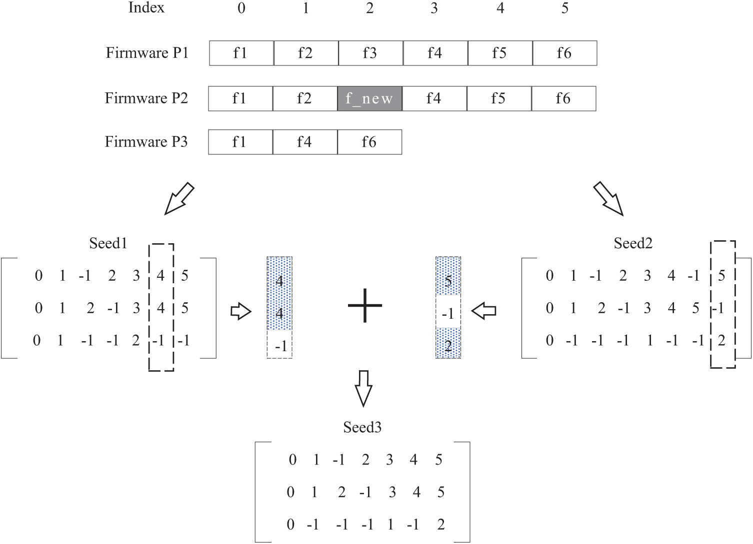
Figure 3: Seed generation based on trusted base point

4.2 Trusted Base Point Management

Since selecting trusted base points filters the columns with high similarity in the function matching matrix, each generated seed can extract trusted base points. Given that both feature similarity Simfea′ (Eq. (8)) and non-empty similarity Simfea_ne (Eq. (10)) can be used to measure function similarity, we manage the trusted base points in three levels: confident trusted base points, stable trusted base points and suspected trusted base points.

4.2.1 Confident Trusted Base Points

For a function matching matrix A with a column Aj={a1,j,a2,j,...,aN,j}, Aj is stored as a confident trusted base point if the following conditions are satisfied:

(1)   Its feature similarity satisfies Simfea′(Aj)>δ;

(2)   For any column Ah′={a(′1,h),a(′2,h),...,a(′N,h)} that has been stored as a confident trusted base point, we have Ah′≠Aj;

(3)   For any column Ah′={a1,h′,a2,h′,...,aN,h′}, any non-empty index in column Aj(ai,j>−1,1≤i≤N,i∈Z) satisfies ai,j≠ai,h′ for any column Ah′={a1,h′,a2,h′,...,aN,h′} that has been stored as a confident trusted base point.

In this paper, the maximum feature similarity is 1, and considering the slight difference of floating-point numbers in operation, δ is taken as 0.99. The discriminative condition of the above confident trusted base point can be understood as follows: any function of any firmware in the multi-firmware comparison will not belong to the sequence of two sure confident trusted base points at the same time, and the similarity of the sequence of the confident trusted base point to which it belongs should be extremely high. Due to the high similarity of the confident trusted base points, if a function belongs to a confident trusted base point, then any relevant records containing the stable trusted base points and suspected trusted base points of that function will be cleared.

4.2.2 Stable Trusted Base Points

The similarity of stable trusted base points is lower than that of confident trusted base points and higher than that of suspected trusted base points. Stable trusted base points include two main cases:

•   In the process of adding confident trusted base points, if a column Aj={a1,j,a2,j,...,aN,j} in the function matching matrix A satisfies the above conditions (1) and (2), but not (3), then Aj is stored as a stable trusted base point;

•   For a column Aj={a1,j,a2,j,...,aN,j} in the function matching matrix A, its non-empty similarity is satisfied if Simfea_ne′(Aj)>ϵ.

In this paper, the maximum non-empty similarity is 1, considering the slight difference of floating-point numbers in the operation process. Therefore, ϵ is taken as 0.99.

4.2.3 Suspected Trusted Base Points

For a column Aj={a1,j,a2,j,...,aN,j} in the function matching matrix A, if Aj does not satisfy the conditions of constituting a confident trusted base point and a stable trusted base point, but its feature similarity satisfies Simfea′(Aj)>η, then Aj is stored as a suspected trusted base point. In this paper, η takes the value of 0.5 when 4 sequences are compared. For the function matching matrix with different numbers of sequences and containing different amounts of empty spaces, the expectation of feature similarity of its single column is not the same. In general, the more the number of sequences, the lower the feature similarity of the single column in the early stage of seed generation. Therefore, increasing the value of η as the number of rounds of population renewal increases may be a more reasonable approach. However, we can not perform multi-firmware comparison due to the large amount of memory required when the number of sequences is high. The experiments in this paper involve small-scale multiple sequence comparisons, and the effect of the strategy without η-value changes has been acceptable.

4.2.4 Trusted Base Points Updating

Since each seed can generate a trusted base point, the number of trusted base points will increase as the number of population optimization rounds increases. Therefore, the stored trusted base points need to be updated. The update strategies are different for the three types of trusted base points.

•   Confident Trusted Base Points. Make sure that no function of any firmware belongs to more than one confident trusted base point at the same time, and if this happens, change the corresponding confident trusted base point to a stable trusted base point.

•   Stable Trusted Base Point. There is no restriction on the stable trusted base point for a function. A function can belong to more than one stable trusted base point simultaneously. However, considering the efficiency of implementation, a function that belongs to a different stable trusted base point only retains the highest feature similarity of several. This paper takes the value of 5.

•   Suspected Trusted Base Points. The suspected trusted base point themselves contain a large number of false matches due to the high probability of conflict between suspected trusted base points (see Section 4.3.2 for details). The saved results should be discarded periodically. For the suspected trusted base point, the selection strategy in this paper is to discard the suspected trusted base point with feature similarity lower than 0.8 every 3 rounds.

4.3 Seed Construction Methodology

The essence of population generation is to repeat the seed generation. As long as the seed generation method is straightforward, population generation can be completed. The seed construction based on trusted bases consists of three parts: trusted base point selection, ranking, and seed generation.

4.3.1 Trusted Base Point Selection

Due to the large number of three types of trusted base points stored, it is necessary to select the base points in the process of use. Trusted base point selection is to control the number of selected base points. We randomly choose all of the confident trusted base points at each seed generation, 50% of the stable trusted base points, and 1% of the suspected trusted base points to guide the seed construction.

4.3.2 Trusted Base Point Ranking

After completing the initial filtering of trusted base points, it is necessary to rank them to reduce the difficulty of subsequent seed construction. For two trusted base points Aj={a1,j,a2,j,...,aN,j} and Ah={a1,h,a2,h,...,aN,h}, if ai,j≠−1∧ai,h≠−1 (1≤i≤N), and ai,j<ai,h are satisfied, then the base point Aj is smaller than Ah, which is denoted as Aj<Ah. That is, the non-empty term in one base point is also non-empty in the corresponding term in another base point, and the former value is smaller than the latter, and all non-empty terms in the base point satisfy the above condition.

Based on the above criteria, the selected trusted base points can be ranked. However, there are still two cases that need to be handled: Case (1), No order relation. For two trusted base points Aj={a1,j,a2,j,...,aN,j}, Ah={a1,h,a2,h,...,aN,h}, there is no case that ai,j>−1∧ai,h>−1,1≤i≤N. Case (2), Ranking contradiction. If two trusted base points Aj={a1,j,a2,j,...,aN,j} and Ah={a1,h,a2,h,...,aN,h}, at ai,j>−1∧ai,h>−1 (1≤i≤N), if one of the following two conditions is satisfied: there exist both cases where ai,j<ai,h and cases where ai,j>ai,h. And there exists the case where ai,j=ai,h. Then the ranking contradiction is considered.

For the case of no sequential relationship, since the two basis points are not divided into sizes, the size of the two basis points is determined randomly in the sorting process. For the case of contradictory ranking, we eliminate one of the conflicting basis points, and the principle of elimination is as follows:

•   If the two bases are both confident trusted base points or suspected trusted base points, one base point is retained, and the other is deleted based on the similarity of the two bases.

•   If both base points are stable trusted base points, one base point is retained, and the other one is deleted based on the similarity of the non-null features of both base points.

•   If two base points are not of the same type, and one of them is a confident trusted base point, keep the confident trusted base point and delete the other one.

•   If two base points are not of the same type, and one of them does not exist, one is retained, and the other is deleted based on the similarity of the two bases.

Based on the above principle, the selected trusted base point are eliminated and sorted to form an ordered sequence of trusted base points from smallest to largest.

4.3.3 Seed Generation

After obtaining the ordered sequence of trusted base points, we transform the generating the seeds (i.e., function matching matrix) into filling the index values segment by segment. For any two adjacent trusted base points in the ordered sequence of trusted base points, take Aj={a1,j,a2,j,...,aN,j} and Aj+1={a1,j+1,a2,j+1,...,aN,j+1} as examples, a set can be formed intervals (a1,j,a1,j+1), (a2,j,a2,j+1),..., (aN,j,aN,j+1). Here, it is assumed that the boundary of each interval is non-negative (i.e., the trusted base point has a matching function at the corresponding firmware), because even if the boundary is negative (the corresponding firmware has no matching function at the trusted base point), the maximum and minimum limits of index values can be obtained by retrieving the ordered sequence of trusted base points forward and backward. After obtaining the intervals (a1,j,a1,j+1), (a2,j,a2,j+1), ..., (aN,j,aN,j+1), it is only necessary to determine the maximum interval length and the proportion of empty space-filling to randomly generate the correspondence of multiple firmware functions in an interval. The intervals cut from the ordered sequence of trusted bases are filled one by one and combined to generate new seeds. The filling process is illustrated in Fig. 4.

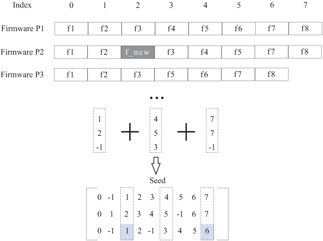
Figure 4: Example of interval filling between bases

Suppose there are three firmwares P1, P2, P3, whose functions correspondence as shown in Fig. 4, and after several rounds of analysis, three trusted base points {1,2,−1}, {4,5,3}, {7,7,−1} are obtained. At this point, P1 is partitioned into three intervals [0,1), (1,4), (4,7); P2 is partitioned into three intervals [0,2), (2,5), (5,7); P3 is partitioned into two intervals [0,3), (3,6] because some of the trusted base points do not correspond to functions. Assuming that the number of columns to be filled between any two neighboring trusted bases is 2, the maximum interval length. There is no requirement for the maximum interval to be filled with empty spaces. The seeds in Fig. 4 can be generated. For example, for the trusted base points 4,5,3, 7,7,−1, the length of the largest interval (4,7) is 2; at this time, there is only one number in the interval (5,7) of firmware P2, which needs to be inserted into the empty space; while for firmware P3, the last number in the interval (3,6] is filled into the trusted base point because of the empty space of the trusted base point. The remaining part still has two numbers still need to be filled. It should be noted that the percentage of empty spaces filled for each firmware is based on the difference between the number of columns of the function matching matrix and the number of columns of the individual firmware, as specified in Section 2.1, where the number of columns of the function matching matrix is greater than the maximum number of firmware functions and less than the sum of all firmware functions.

5  Population Generation Method Based on Local Optimal Solution

We cut each seed of the existing population into several intervals according to the same criteria and combine the optimal solutions of each seed in each interval to form a new population. As shown in Fig. 5, two seeds Seed1 and Seed2 are obtained for several firmware sequences. Seed2 is divided by the same interval as Seed1 to form two local solutions that can be used to generate new seeds, consisting of {−1,2,−1}T, {2,−1,−1}T, {3,3,1}T columns and {4,4,−1}T, {−1,5,−1}T, {5,−1,2}T columns respectively. We find that the second local solution of Seed1, {4,4,−1}T, {5,5,−1}T and the first local solution {−1,2,−1}T, {2,−1,−1}T, {3,3,1}T of Seed2 are the local optimal choices, so we can form Seed3 by splicing the above two local optimal solutions and filling the other parts to generate a new function matching matrix.

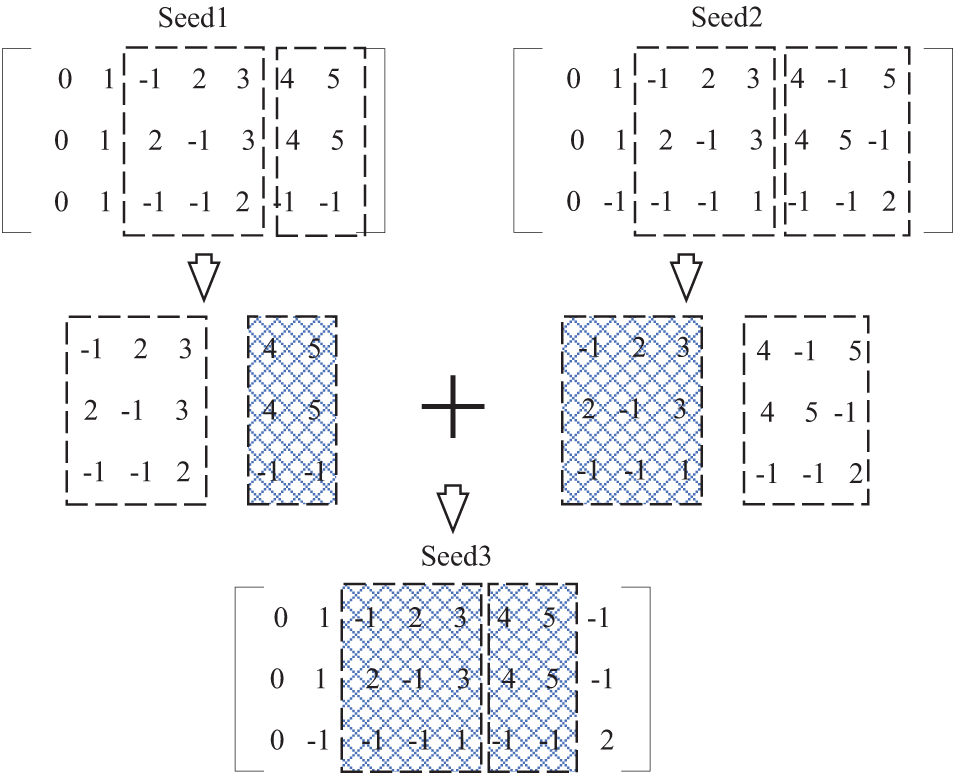
Figure 5: Example of seed generation based on local optimal

5.1 Interval Segmentation

The purpose of interval segmentation is to provide uniform criteria for selecting local optimal solutions among different seeds and provide a crossover between seeds. With interval segmentation, the function matching matrix can be partitioned into several small matrices representing the local function correspondence of the firmware.

For several function matching matrices (i.e., populations) formed by N firmwares, one firmware is first selected as the benchmark from among N firmwares for partitioning the interval, assuming that the sth firmware is chosen as the benchmark and its number of functions is ls. If the seed is to be divided into M intervals, then M−1 non-repeating positive integers less than ls are randomly selected to form the sequence B1, B2...,BM−1. from smallest to largest.

For each function matching matrix in the population (take an N ∗ L matrix A as an example), A can be cut into M small matrices Apiece,h with size N∗mh, where A=(ai,j),h∈Z(0≤h≤M−1). Apiece,h=(bh,i,j) is satisfied: (1) Σh=0M−1mh=L; (2) x=0 when h=0; x=Σk=0h−1mk when h>0; (3) bh,i,j=ai,j+x,0≤i<N,0≤j<mh; (4) When h>0, as,x=Bh. That is, any column in matrix A can find the same column in the unique small matrix Apiece,h; when 0<h<M−1, each small matrix Apiece,h contains all functions whose index value of the sth firmware is in the interval [Bh,Bh+1).

Based on the above conditions, we can continue adding the requirements to limit the sequence B1,B2,...,BM−1. The difference between two adjacent integers remains unchanged, and the interval is divided according to this condition, except for the first and the last interval, which can ensure a relatively stable span of the interval.

An example of interval segmentation is shown in Fig. 6. The two examples of interval segmentation are based on row 2, which represent the two cases of random interval segmentation (i.e., the number of functions in each interval of the base file is random) and equidistant interval segmentation (i.e., the number of functions in each interval of the base file is equal except for the first and last intervals). In this paper, we chose the method of isometric interval division in the experiment, and the interval size was set as 5.

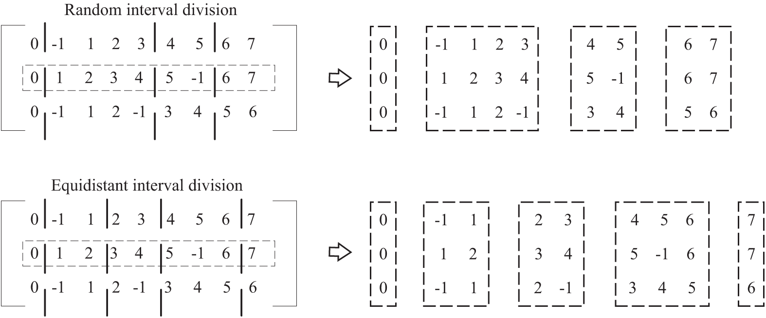
Figure 6: Example of interval division

5.2 Seed Construction

With interval segmentation, several intervals can be formed based on a specific firmware, and any seed in the population can create a corresponding small matrix (local solution of multiple sequences) based on a specified interval. Ideally, a local optimal solution can be selected among the small matrices obeying the same interval. The local optimal solution in each interval can be spliced to generate a better new seed. As shown in Fig. 5, the first row of the seed is the base, and the second interval is [4,6) through the interval division. Thus Seed1 forms the small matrix {4,4,−1}, {5,5,−1}, and Seed2 forms the small matrix {4,4,−1}, {−1,5,−1}, {5,−1,2}; by comparing the two small matrices (e.g., adaptation value), it is determined that the small matrix of Seed1 is the local optimal solution. Therefore, it is used for the generation of Seed3. However, there are still 2 problems to be solved in seed construction.

5.2.1 Local Optimal Solution Selection

When picking small matrices within the same interval, whether a small matrix is ideal as a local solution can be evaluated by following the fitness function in Section 3.2. However, the local solution with the highest adaptation score is not guaranteed to match the functions between firmwares because the function between firmwares is often deformed due to the upgrade. Therefore, in practice, one of the local solutions with the highest adaptation score should be selected for subsequent seeding instead of just selecting the solution with the highest adaptation value. By doing so, we can increase the possibility of finding the actual matching result of the deformation function. In general, the top 5% to 10% of the local solutions are selected based on their adaptation scores, and the selection is proportional to the adaptation scores of the local solutions. The local solutions chosen by the above method are referred to as local optimal solutions in the following. The proportion of 5%–10% is chosen because the number of individuals in the optimal population is above 100 (usually 130), and there will not be less than one local solution to choose from.

5.2.2 Local Optimal Solution Splicing

After the local optimal solutions are selected for each interval, each local optimal solution is sorted according to the order of the intervals. Then the local optimal solutions are stitched together to form a new seed. However, two cases (i.e., interval interruption and interval overlap) cannot be directly spliced between the local optimal solutions. Fig. 7 shows the local optimal solutions of the three intervals with the firmware in row 2 as the base, and the shaded area shows the interval interruption and interval overlap. Interval interruption is where a function of a firmware line is not included in any of the local optimal solutions. It is common for functions that are unique to that firmwares and functions that fail to match. For example, as shown in Fig. 7, the first line of firmware is missing the function with index 4. In this case, it is straightforward to fill the interval between two adjacent locally optimal solutions by analogy with the filling method in Section 5.2. The interval overlap is when the functions of a firmware line appear in the adjacent local optimal solutions simultaneously. In Fig. 7, the function with the firmware index 6 in the first row appears twice. There are two ways to deal with interval overlap:

•   row-by-row random discarding. Two local optimal solutions of a row of overlapping function index interval [ia,ib], where ia,ib∈Z,0≤ia≤ib. Randomly select an integer i′ belonging to the interval. The former of the two local optimal solutions will set the part of the overlapping interval of the row with an index value less than or equal to i′ to null (the value is changed to −1). The former will set the part of the overlapping interval of the row with the index value. The latter will empty the part of the overlapping interval whose index value is greater than i′.

•   overall random discarding. The fitness value of the two local optimal solutions is calculated, and one of them is selected randomly according to the fitness value. The other is discarded and does not participate in the local optimal solution splicing. The interval interruptions caused by discarding the local optimal solution are treated as interval interruptions.

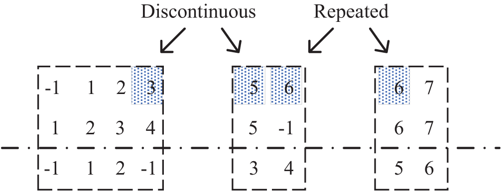
Figure 7: Discontinuous interval and repeated interval

In practical experiments, the overall random discarding method has good experimental results. See Section 6.4.2 for details.

6  Evaluation

In this Section, we first introduce the experiment environment, dataset, and evaluation metrics and baseline. Then, we study the effect of trusted base points on multi-firmware comparison and the effect of the local optimal solution splicing method on the multi-firmware comparison. Finally, we compare our solution with Bindiff (version 5) and the string-based method, and we manually verify the multi-firmware comparison effect of our approach. Specifically, our evaluation aims to answer the following research questions (RQ).

•   RQ1: Whether the trusted base point is effective for multi-firmware comparison?

•   RQ2: Whether the local optimal solution splicing is effective for multi-firmware comparison?

•   RQ3: How effective is our solution compared with state-of-the-art works for multi-firmware comparison?

6.1 Experiment Environment

The experimental environment consists of an Intel Xeon Gold 6150 CPU @2.70 GHz processor, 128 GB RAM, Samsung T5 SSD 2 TB hard disk. We use the IDA Pro to preprocess the firmware and implement the proposed method with Python 3.7.

6.2 Dataset

To demonstrate the effect of our solution. we select the Cisco C2600, C1800 series firmwares as our dataset. The two series of firmwares have different instruction sets. The number of functions in the firmware is large, and the firmware is monolithic executables rather than multiple files packaged and compressed, which has the value of analysis. Specifically, to study the effect of trusted base points on the multi-firmware comparison, we select four firmware, i.e., c1841-advipservicesk9-mz.124-17, c1841-advipservicesk9-mz.124-22.t, c1841-advipservicesk9-mz.124-22.t, c1841 advsecurityk9-mz.124-24.t5, and c1841-broadband-mz.124-16. The number of seeds for the optimal population is set to 130, and the number of seeds generated by each of the three population update methods is 70 (210 in total). The number of iterations in this experiment was set to 20.

In addition, we select four other firmwares to study the effect of local optimal solution splicing and compare with baseline works, including c2600-ipbase-mz.123-6f, c2600-ipbase-mz.123-25, c2600-ipbase-mz.124-19, and c2600-ipbase-mz.124-25c. The number of seeds for the optimal population is set to 130, and the number of seeds generated by each of the three population update methods is 70 (210 in total). The number of iterations in this experiment was set to 200 rounds.

6.3 Metrics and Baseline

Due to the difficulty of multiple sequences matching itself, the fact that some of the firmware functions in the matching results are set to correspond to empty bits does not mean that the function does not correspond to the matching function but may not find the actual matching result. Based on this consideration, only the non-empty matches in each row of the function matching matrix are considered when designing the similarity of matching results.

The seed with the highest adaptation (function matching matrix) needs to be analyzed to verify the correctness of the function correspondence in the function matching matrix. Since we do not have the source code for these firmwares, we cannot build ground truth, so we use the following evaluation methods to evaluate our approach.

Metric I: Similarity of matching results. The similarity of matching results. N firmwares using method X for multiple sequence matching formed a function matching matrix A, the size of matrix A is NxL, and another M pairs of firmwares obtained M dual sequence comparison results by method Y. The similarity of matching results between method X and method Y, Ms(X,Y), is shown in Eq. (11).

Ms(X,Y)=(Σi=1Lτi∗Cki2)/(Σi=1Lςi∗Cki2)τi={xi/yi,yi>00,  yi=0ςi={1, yi>00,yi=0(11)

where ki denotes the number of non-empty items (value non–1) in the i-th column of matrix A, which cumulatively can form Cki2 non-empty dual-sequence matching results, yi denotes the number of non-empty item matching results in the i-th column that can be compared with M dual-sequence comparison results, and xi denotes the number of yi results in which the two methods agree.

Metric II: Precision. As shown in Eq. (12), where TP is a true positive result, and FP is a false-positive result.

precision=TP/(TP+FP)(12)

In this paper, we do not use the precision directly for evaluation mainly based on the following considerations: without the source code of firmware, it is not possible to determine whether the function matches are correct or not, and due to a large number of firmware functions and the significant time cost of manual analysis, it is not reliable to use the precision of the sampled results as the precision rate of the multi-firmware comparison results, and the value can only be used as a reference. Therefore, the precision of the analysis results can be compared with previous dual-firmware comparison methods or tools with high precision. If the similarity of the matching results is high, the accuracy of the analysis results is considered close to that method.

Baseline. In this paper, we choose Bindiff and string-based method as the baseline. The similarity between the proposed method and Bindiff is evaluated by using the similarity of matching results, supplemented by the precision analysis, obtained by sampling the results of multi-firmware matching and then manually verifying them.

The string-based matching is a classical method for constructing function correspondence by extracting the strings referenced by functions within the firmware to establish the function correspondence between firmwares. Although the similarity of matching results can be used to measure the degree of approximation between the proposed method and Bindiff, Bindiff itself has miss-matching cases. Meanwhile, string-based matching is less likely to have miss-matching instances, so the similarity of matching results with strings can be used as a supplement to measuring the operation effect of our solution. Therefore, the similarity of string-based method can be used as a supplement to measuring the effectiveness of our solution.

6.4 Results

6.4.1 Effect of Trusted Base Points on Multi-Firmware Comparison

To answer the RQ1, we study the effect of the number of trusted base points and the number of empty spaces on the multi-firmware comparison. The experiment is performed in 7 groups. Each group is pre-selected with a certain number of trusted base points (the number of trusted base points is from manual analysis, more than 10,000) to simulate the effect of our solution in Section 4.

Since it is a 4-firmware comparison, there are three cases of trusted base point according to the number of nulls: no null, 1 null and 2 nulls. The sets of trusted base points provided by the 7 sets of experiments are as follows: (TB1) randomly select 10 non-empty trusted base points. (TB2) randomly select 100 trusted base points, where the ratio of no null, 1 null and 2 null trusted base points is 1:1:1. (TB3) randomly select 100 trusted base points, among which the ratio of no null, 1 null and 2 nulls trusted base points is 1:1:2. (TB4) randomly select 100 trusted base points, among which the ratio of no null, 1 null and 2 null trusted base points is 2:1:1. (TB5) randomly select 1000 trusted base points, among which the ratio of no null, 1 null and 2 null trusted base points is 1:1:1. (TB6) randomly select 1000 trusted base points, among which the ratio of no null, 1 null and 2 null trusted base points is 1:1:2. (TB7) randomly select 1000 trusted base points, among which the ratio of no null, 1 null and 2 null trusted base points is 2:1:1.

The experimental results are shown in Fig. 8. As shown in Fig. 8, both the fitness values and similarities increase with the number of iterations. Increasing the number of trusted base points also leads to better results: for fitness, increasing the number of trusted base points leads to higher fitness values, while for both similarities, increasing the number of trusted base points leads to more minor fluctuations in similarity values. For the proportion of trusted base points of different null types, the fitness value is higher when the ratio of null-free trusted base points is higher. As for the similarity, the experiment is at the early stage of training, and the similarity fluctuates a lot, so we can only see that the trend of the mean increase is the same as a whole, and we cannot determine which ratio has a more significant effect on the similarity.

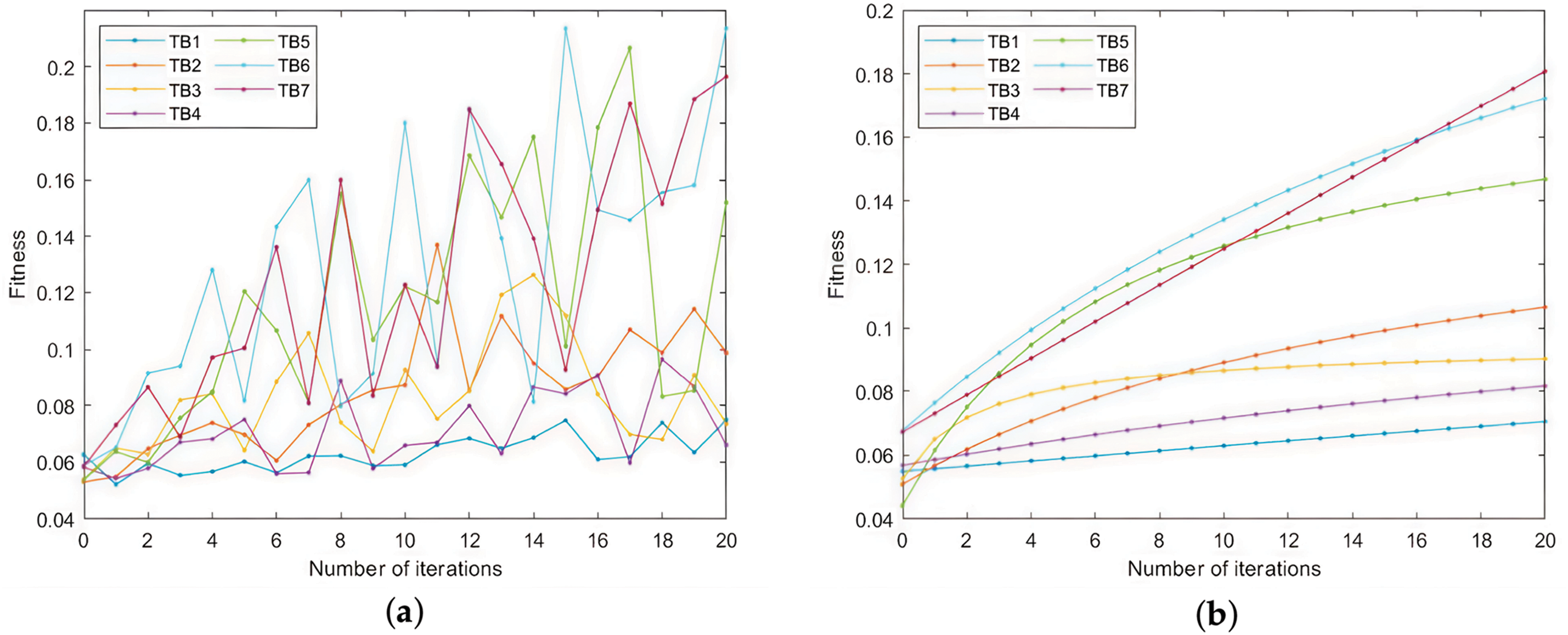
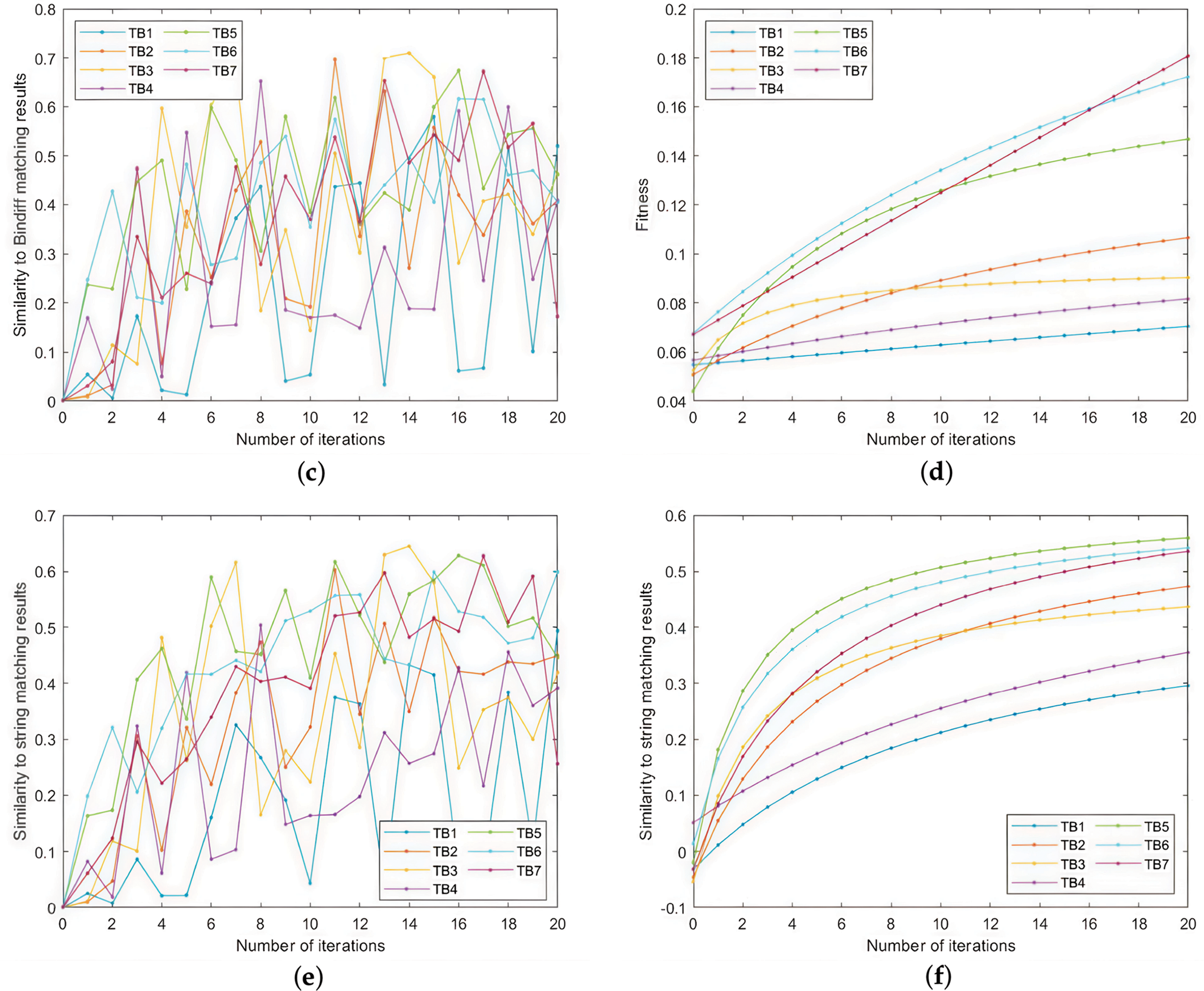
Figure 8: The influence of trusted base points on the multi-firmware comparison. (a) The mean fold of fitness for each round of seeds during 20 iterations; (b) The mean of fitness; (c) The mean fold of similarity to Bindiff for each round of seeds during 20 iterations; (d) The mean of fitness; (e) The mean fold of the similarity between the seeds and the string-based matching results for each of the 20 iterations; (f) The mean of fitness

6.4.2 Effect of Local Optimal Solution Splicing Method on Multiple Sequence Comparison

In this part, we try to answer the RQ2. Section 5.2 proposes two local optimal solution splicing methods for the case of overlapping intervals: row-by-row random discarding and overall random discarding. The result is shown in Fig. 9. Fig. 9a shows the fitness scatter plot of the optimal population. Each column of the scatter represents the fitness value of each individual in the optimal population after that round of iteration. The orange nodes indicate the overall random discarding. The blue nodes indicate the row-by-row random discarding. Fig. 9b shows the mean values of the fitness of the optimal population in each iteration. The red line indicating the overall random discarding and the blue line indicating the row-by-row random discarding.

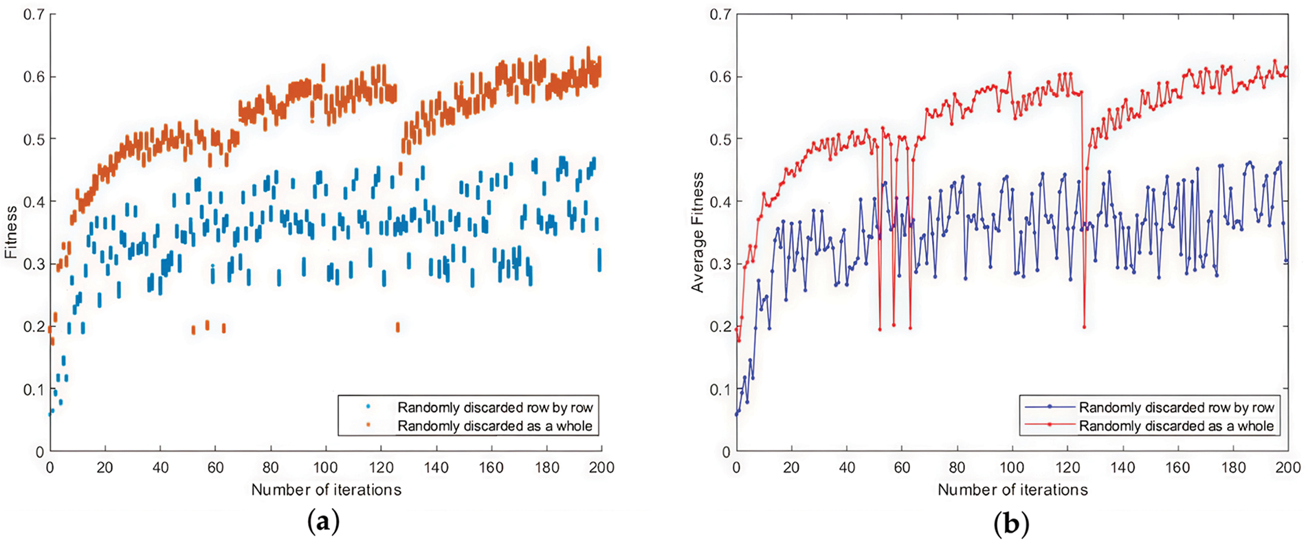
Figure 9: Comparison of local optimal solution combining methods: (a) The fitness scatter plot of the optimal population; (b) The mean values of the fitness of the optimal population in each iteration

The experiments show that the overall random discarding is more effective than the row-by-row random discarding. The former has a significantly larger fitness value than the latter, with less fluctuation. There are several reasons for this result. One of the main reasons is that the row-by-row random discarding is likely to destroy the correct function correspondence in the local optimal solution because the overlapping of the local optimal solution is randomly replaced, which leads to the decrease of the similarity of the local optimal solution after splicing. In contrast, the overall random discarding does not cause such damage. The above situation may arise only from a few mismatched functions with high similarity. If the frequency of interval overlap between local optimal solutions and the size of the overlap can be controlled, then the row-by-row random discarding should also be effective. Therefore, the row-by-row random discarding can be tried to deal with the overlap problem at a later stage of the multi-sequence matching, i.e., after most of the correspondences between the firmware functions have been correctly constructed.

6.4.3 Adaptation and Similarity of Matching Results

To answer the RQ3, we compare our solution with Bindiff (version 5) and string-based method.

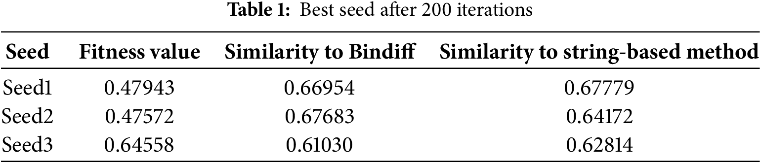
Fig. 10 shows the evolution of the optimal population for the 200 iterations of the 4-firmware. Fig. 10a shows the scatter plot of the optimal population. The scatter points in each column represent each individual in the optimal population after that iteration. The yellow nodes indicate the fitness values. The blue nodes indicate the similarity of the seeds with Bindiff matching results. The orange nodes indicate the similarity of the seeds with string-based matching results. Fig. 10b shows the mean values of the best populations in each iteration, the black line shows the mean value of fitness, the red line shows the mean value of similarity with Bindiff matching results, and the blue line indicates the mean value of similarity with string-based matching results. As shown in Fig. 10, with the increase of the number of iterations, the best populations are continuously updated. The overall trends of fitness, similarity with Bindiff matching results, and similarity with string-based matching results are consistent. The values reach above 0.5 and stabilize after about 70 iterations. It should be noted that there are four large fluctuations in Fig. 10 because the experiment was not completed in one time, and the program had to be rerun based on the results at that time due to the interruption of the experiment caused by the power failure. In fact, from the perspective of smoothing the data, it is sufficient to exclude the data of these 4 times, even if keeping or excluding the data of these 4 times does not affect the effectiveness of the argument of this paper. However, we realize that the evolutionary algorithm has some robustness in the iterative process itself, and therefore, we choose to keep such original data. After 200 iterations, the optimal population has three seeds with the largest of the three taken values, as shown in Table 1. It can be seen that it is a reasonable choice to use the fitness value of the proposed method to measure the seeds, and the seeds with the higher values of all the three kinds of values (i.e., Seed3) can be obtained. The experiment shows that the similarity of matching result between our solution and the Bindiff is above 60%.

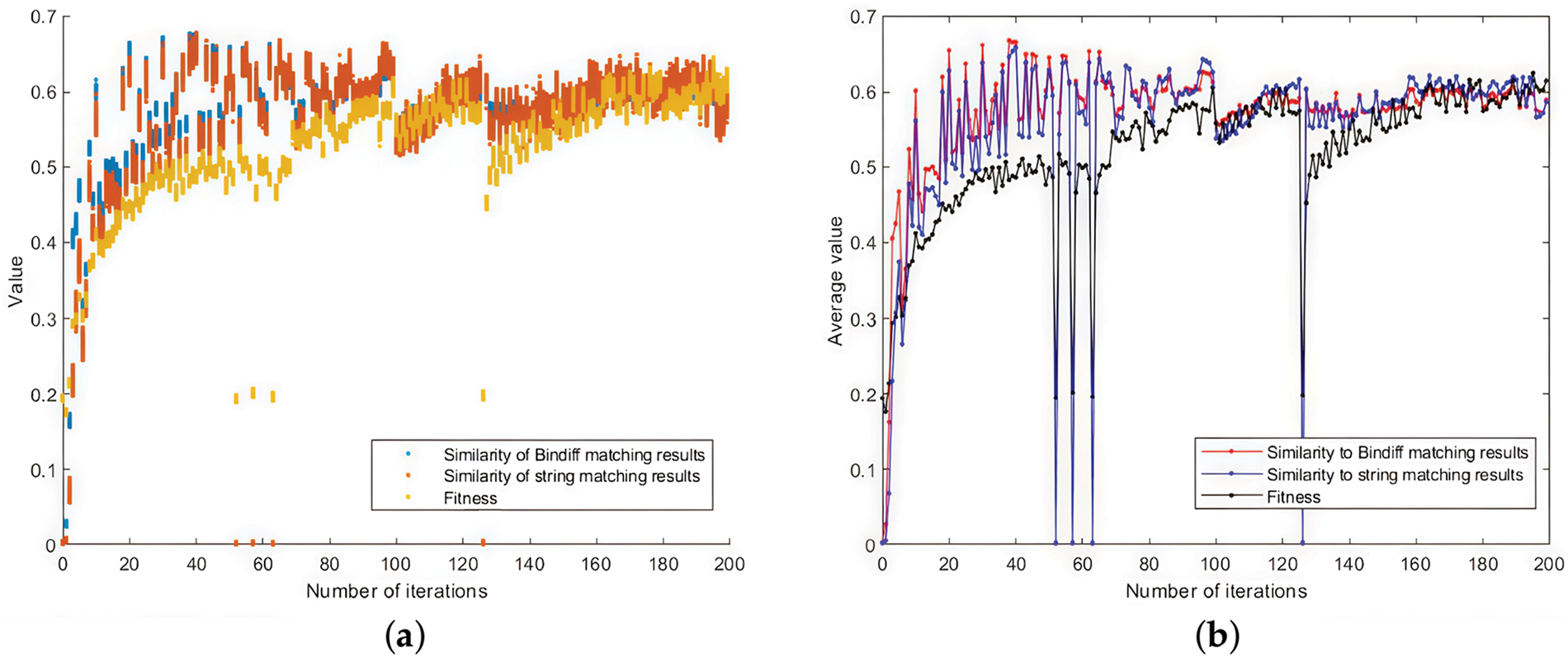
Figure 10: P4 Sequence comparison effect: (a) The evolution of the optimal population for the 200 iterations of the 4-firmware; (b) The mean values of the best populations in each iteration

6.4.4 Sampling and Manual Verification

To determine the effectiveness of the proposed method, the results of the 4-firmware comparison are sampled and manually checked.

The sampling consists of four cases, which are: (Case 1) the method of this paper is consistent with Bindiff; (Case 2) the method is not compatible with Bindiff; (Case 3) the method is consistent with the string-based matching result; (Case 4) the method is not consistent with the string-based matching result.

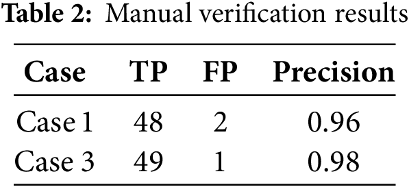
For each case, 50 cases were selected and 200 cases in total. For Case 1 and Case 3, the results of the manual verification are shown in Table 2. It can be seen that the sampling accuracy of this method is at least 96% when it agrees with the Bindiff matching result or the string-based matching result. The similarity of the matching results proposed in this paper is a measure of the similarity between this method and other methods in the matching results.

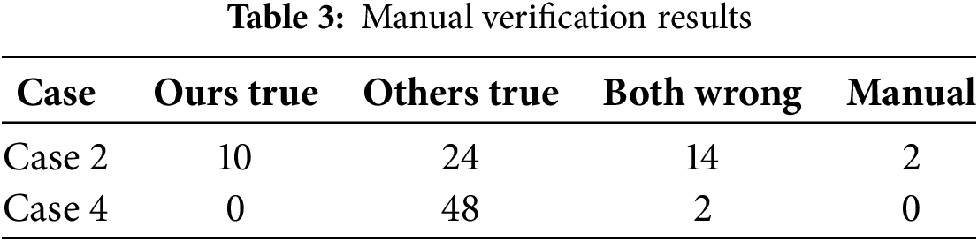
For Case 2 and Case 4, the manual verification results are shown in Table 3. It can be seen that the results of the proposed method are not satisfactory when they are not consistent with Bindiff matching results or string-based matching results. The main reason is that this method is multi-sequence matching, while the other method is dual-sequence matching, and the difficulty of matching is different. In terms of string comparison, not all functions have strings, and not all functions with strings are sampled, so the sample coverage is not wide enough. Therefore, to evaluate the overall accuracy, Bindiff is preferred as a reference, and the matching result of this method can reach 66.4% accuracy under this condition (Table 1, Seed3, 0.6103 * 0.96 + 0.3897 * 0.2).

Based on the present results, it can be seen that increasing the similarity of matching results of our solution can indeed achieve higher accuracy. In addition, it is reasonable to use the similarity of matching results as the evaluation index at this stage, which can make up for the shortage of manual verification.

7  Discussion

7.1 The Analysis of Time-Space Overhead

Our solution solves the problem of constructing function correspondence between multiple firmwares, which requires an analysis of its time-space overhead.

Assuming that there are N firmwares for multi-firmware comparison and li is the number of functions of the i-th firmware, 1≤i≤N. For the traditional dual-firmware comparison method, if the function correspondence is constructed in any two of these N firmwares, at least CN2 dual-firmware comparisons should be performed to observe the experimental results more comprehensively (the transferability contradiction of the dual-firmware matching results). In this case, it is necessary to increase the number of firmware comparison analyses for the transferability contradiction of the dual firmware comparison results. For example, there are firmware P1, P2, P3 and functions f1, f2, f3, f4 satisfying f1∈P1, f2∈P2, f3∈P3, f4∈P3; suppose the functions f1, f2, f3 have correspondence (e.g., they are all library strcpy functions), but using the traditional dual firmware matching However, using the traditional two-firmware comparison method for P1, P2, and P3, it is entirely possible that f1, f2 match (P1 vs. P2), f1, f4 match (P1 vs. P3), and f2, f3 match (P2 vs. P3); at this point, in order to correct the results, it is inevitable to increase the inter-firmware comparison, and CN2 only estimates the lower limit of the number of firmware comparisons.

Now we have the assumption that the average number of functions of firmware is m, the space occupied by a single function is Spacef, and the time overhead of computing similarity between two functions is Tsim. The space overhead of CN2 dual firmware comparisons is O(Spacefx(N−1)xΣi=1Nxli). Since Spacef is a constant, its space complexity is O(Nm2). The time similarity analysis is relatively complicated because the methods used in different studies are different, especially some of them are graph isomorphism and propagation algorithms, so it is difficult to determine the average time complexity; however, it can be roughly understood that the time overhead of a pair of firmware for comparison is between O(mTsim) and O(m2Tsim). Since Tsim is a constant, then, CN2 times of double firmware The time complexity of the comparison is between O(N2m) and O(N2m2). For this method, the function matching matrix A=(aij), satisfies 1≤j≤l, max(li)≤l≤Σi=1Nxli. It can be seen that the space overhead of a seed is O(SpacefxNxl), and the space complexity is between O(mN) and O(mN2). Since, in practice, the number of matrix columns does not reach 2 times max(li), the space overhead is biased towards O(mN). Assuming that the population size of this method is c, the space overhead is between O(cmN) and O(cmN2), as long as c is much smaller than m (which is typical for firmware with hundreds of thousands of functions), the space overhead of this method can be smaller than the traditional dual firmware comparison.

For the time complexity, since this paper adopts Eq. (3) to calculate the single column similarity, the time overhead of one column function in the matrix is O(N2Tsim). The time overhead is between O(cmN2) and O(cmN3) by combining the number of populations and seed length. However, further analysis is needed regarding the time complexity. First, an evolutionary algorithm is a method to randomly search for the optimal solution, and the traditional approach is considered optimal when solved once. In contrast, the method in this paper requires multiple solutions, which is not comparable. A one-time solution cannot solve the mismatching problem pointed out in this section, and it is impossible to estimate how many times the optimal solution can be obtained. Second, the time overhead of the method in this paper is between O(cmN2) and O(cmN3), but this is fluctuated by the matrix length, and since the general matrix length does not reach Nm, but slightly higher than max(li), the time overhead of this paper is closer to O(cmN2). In the experiments in Section 6, the seed generation is 210 per round at maximum and 200 at most. In the experiments in Section 6, the cumulative number of seed generation is less than 100,000, therefore, in practice, c is much smaller than m, and the time overhead O(cmN2) is smaller than O(N2m2).

7.2 The Importance of Trusted Base Points in Firmware Security

Trusted base points are critical in firmware security, providing stable reference points for function matching across different firmware versions. This stability is essential for detecting security vulnerabilities and malicious code, as security analysis often requires comparing multiple firmware versions. For example, in cross-version comparisons, trusted base points ensure consistent function matching even when firmware undergoes updates or modifications. This consistency is vital for identifying subtle changes that may indicate malicious code insertion or vulnerability exploitation. Moreover, trusted base points help reduce false positives and false negatives in security assessments. By offering a stable reference, they enhance the reliability of automated security tools, making them more effective in detecting both known and unknown threats. This is particularly important in environments where firmware updates are frequent. Trusted base points also support complex matching scenarios, such as cross-version and cross-architecture comparisons. These scenarios are crucial for identifying sophisticated attack patterns that may span multiple firmware releases or target different hardware platforms. For instance, attackers might exploit vulnerabilities in older firmware versions and propagate them to newer versions. Therefore, cross-version analysis is indispensable for comprehensive security auditing.

In summary, the proposed method not only reduces the time and space overhead compared to traditional dual firmware matching methods but also integrates trusted base points to enhance the robustness and efficiency of firmware security analysis. This combination of performance optimization and security reliability makes our approach particularly suitable for real-world firmware ecosystems where both efficiency and security are paramount.

8  Related Work

Binary matching techniques have been studied extensively in the past, and this section summarizes the research related to many-to-many comparisons between programs.

In program analysis, the literature [26] is the earliest study found to compare the similarity of many-to-many programs. This paper extracted the program’s control flow graph (CFG) and combined it with graph coloring techniques to detect the variant worms. The experimental dataset consists of less than 20 MB executable files. Saebjornsen et al. [31] used disassembly instructions as input. After instruction transformation and normalization, it uses a clustering algorithm to evaluate the similarity of instruction sequences, thus realizing binary code similarity evaluation. Although the input is multiple binary code regions, the comparison results are to find the most matching clone instruction sequence to score the similarity rather than construct a functional correspondence. Santos et al. [32] proposed a detection method based on opcode sequence frequency for unknown malware variants. Also, a way is provided to mine the correlation of each opcode to weigh its sequence frequency. The literature [33] aims to perform malicious family categorization of malware; by performing master block extraction of functions to reduce the time overhead of similarity analysis. Although the comparison is many-to-many, the object of the comparison is multiple master blocks of two files, which is essentially a one-to-one comparison of programs. The study in [34] compares at the CFG level obtain semantic meaning to the binary code through dynamic execution behavior to observe changes in the behavior of the underlying malware functionality over time. Jin et al. [35] designed a hashing method that can map the semantic information of functions into corresponding feature vectors and perform function clustering based on the feature vectors to guide finding semantically similar functions in many binary programs. However, to improve identification accuracy, it is necessary to simulate the execution of the basic block to extract the basic block input and output for hashing. Hu et al. [27] extracted the disassembly opcodes of malicious programs used N-gram opcode short sequence features to represent malicious programs, and then used Euclidean distance to calculate the similarity of different programs and used a clustering algorithm to categorize malicious programs. Jang et al. [36] proposed a method for measuring software evolution relationships and two software evolution types. Farhadi et al. [28] mainly detected code clones in malware, including both exact clone detection and imprecise clone detection, defines clones by judging the similarity of consecutive assembly instructions and integrates small clone intervals into large clone intervals by clone fusion. This study mainly focuses on the similarity analysis at the assembly instruction level, which is still a comparison between the two files. Ruttenberg et al. [37] aimed to find the standard function modules (set of functions) among different malware. Through two stages of clustering, the primary function modules in the samples are first clustered into several clusters of basic function modules. Then each sample is carved based on the clusters, and then inter-sample clustering is performed to determine the correlation between samples. Wang et al. [29] propose a jump-aware Transformer-based model, jTrans, which integrates control-flow information into the Transformer architecture to conduct function similarity detection. Their method focuses on one-to-many tasks in this study but can be extended to many-to-many problems by treating each function in the pool as a source function and solving multiple one-to-many problems. Luo et al. [30] propose an intermediate representation function model that lifts binary code into microcode, preserving the main semantics of binary functions through instruction simplification. This approach is designed to facilitate cross-architecture binary code search. Although their method supports many-to-many function similarity analysis, it primarily focuses on measuring the similarity between two given binaries at the function level.

The above study found that previous studies, except for the method [35], could not be used to construct function correspondence between multiple firmwares. This study [35] focused on finding function hash methods, which are relatively expensive to maintain for constantly updated firmware; in particular, the technique requires simulation execution to obtain essential block input-output pairs, which is too much overhead due to a large number of firmware functions (up to hundreds of thousands) and is less feasible for firmware.

Our approach fills the research gap of multi-firmware comparison, reduces the time overhead of using the dual-firmware matching method in the multi-firmware matching scenario, and avoids the contradiction of non-closed matching result transfer based on the transferability of dual-firmware matching result in the multi-firmware matching scenario. In addition, our solution is mainly based on the evolutionary algorithm to adjust the function matching scheme and obtain the optimal matching results of multi-firmware functions. It does not conflict with the method of using function hash to calculate function similarity in the literature [35] and can be used in combination.

9  Conclusion

In this paper, we propose an evolutionary algorithm-based multi-firmware comparison method. First, we transform the multi-firmware comparison problem into a multi-sequence comparison problem and design a fitness function for firmware comparison. Then, we propose a population generation and updating method based on the trusted base point and local optimal solution for firmware and combine the two ways to optimize the optimal population. Finally, we compare our solution with Bindiff and the string-based method. The experiments show that the proposed method outperforms Bindiff and the string-based method. Besides, the more trusted base points, the more nodes are matched without empty space and the best result of the multi-firmware comparison. Our solution is feasible and effective.

While our proposed evolutionary algorithm-based method for multi-firmware comparison has demonstrated significant improvements over existing approaches, several avenues for future enhancement remain. In future research, we will further analyze the characteristics of firmware updates, such as changes in the relative positions of code, to optimize the comparison process.

Acknowledgement: The authors would like to express their gratitude to the editors and reviewers for their detailed review and insightful advice.

Funding Statement: The authors received no specific funding for this study.

Author Contributions: Conceptualization: Wenbing Wang, Yongwen Liu; Investigation: Wenbing Wang; Methodology: Wenbing Wang, Yongwen Liu; Validation: Wenbing Wang; Writing—original draft preparation: Wenbing Wang; Writing—review and editing: Yongwen Liu; Supervision: Yongwen Liu. All authors reviewed the results and approved the final version of the manuscript.

Availability of Data and Materials: Data available on request from the authors.

Ethics Approval: Not applicable.

Conflicts of Interest: The authors declare no conflicts of interest to report regarding the present study.

References

1. Raghunathan K. History of microcontrollers: first 50 years. IEEE Micro. 2021;41(6):97–104. doi:10.1109/MM.2021.3114754. [Google Scholar] [CrossRef]

2. Nino N, Lu R, Zhou W, Lee KH, Zhao Z, Guan L. Unveiling IoT security in reality: a firmware-centric journey. In: 33rd USENIX Security Symposium (USENIX Security 24); 2024; Philadelphia, PA. Berkeley, CA, USA: USENIX Association; 2024. p. 5609–26. [cited 2025 Mar 5]. Available from: https://www.usenix.org/conference/usenixsecurity24/presentation/nino. [Google Scholar]

3. Wu Y, Wang J, Wang Y, Zhai S, Li Z, He Y, et al. Your firmware has arrived: a study of firmware update vulnerabilities. In: 33rd USENIX Security Symposium (USENIX Security 24); 2024; Philadelphia, PA. Berkeley, CA, USA: USENIX Association; 2024. p. 5627–44. [cited 2025 Mar 5]. Available from: https://www.usenix.org/conference/usenixsecurity24/presentation/wu-yuhao. [Google Scholar]

4. Wang J, Zhang C, Chen L, Rong Y, Wu Y, Wang H, et al. Improving ML-based binary function similarity detection by assessing and deprioritizing control flow graph features. In: 33rd USENIX Security Symposium (USENIX Security 24); 2024; Philadelphia, PA. Berkeley, CA, USA: USENIX Association; 2024. p. 4265–82. [cited 2025 Mar 5]. Available from: https://www.usenix.org/conference/usenixsecurity24/presentation/wang-jialai. [Google Scholar]

5. He H, Lin X, Weng Z, Zhao R, Gan S, Chen L, et al. Code is not natural language: unlock the power of semantics-oriented graph representation for binary code similarity detection. In: 33rd USENIX Security Symposium (USENIX Security 24); 2024; Philadelphia, PA. Berkeley, CA, USA: USENIX Association; 2024. p. 1759–76. [cited 2025 Mar 5]. Available from: https://www.usenix.org/conference/usenixsecurity24/presentation/he-haojie. [Google Scholar]

6. Collyer J, Watson T, Phillips I. Faser: binary code similarity search through the use of intermediate representations. arXiv:2310.03605. 2023. [Google Scholar]

7. Wang H, Gao Z, Zhang C, Sha Z, Sun M, Zhou Y, et al. Learning transferable binary code representations with natural language supervision. In: Proceedings of the 33rd ACM SIGSOFT International Symposium on Software Testing and Analysis; 2024; Vienna, Austria. New York, NY, USA: Association for Computing Machinery; 2024. p. 503–15. doi:10.1145/3650212.3652145. [Google Scholar] [CrossRef]

8. Li T, Shou P, Wan X, Li Q, Wang R, Jia C, et al. A fast malware detection model based on heterogeneous graph similarity search. Comput Netw. 2024;254(27):110799. doi:10.1016/j.comnet.2024.110799. [Google Scholar] [CrossRef]

9. Novak P, Oujezsky V, Kaura P, Horvath T, Holik M. Multistage malware detection method for backup systems. Technologies. 2024;12(2):23. doi:10.3390/technologies12020023. [Google Scholar] [CrossRef]

10. Jia L, Yang Y, Li J, Ding H, Li J, Yuan T, et al. MTMG: a framework for generating adversarial examples targeting multiple learning-based malware detection systems. In: Pacific Rim International Conference on Artificial Intelligence; 2023; Jakarta, Indonesia. Berlin/Heidelberg: Springer-Verlag; 2023. p. 249–61. doi:10.1007/978-981-99-7019-3_24. [Google Scholar] [CrossRef]

11. Jia L, Yang Y, Tang B, Jiang Z. ERMDS: a obfuscation dataset for evaluating robustness of learning-based malware detection system. BenchCouncil Transact Benchmarks Stand Evaluat. 2023;3(1):100106. doi:10.1016/j.tbench.2023.100106. [Google Scholar] [CrossRef]

12. Zhang P, Wu C, Peng M, Zeng K, Yu D, Lai Y, et al. The impact of inter-procedural code obfuscation on binary diffing techniques. In: Proceedings of the 21st ACM/IEEE International Symposium on Code Generation and Optimization; 2023; Montréal, QC, Canada. New York, NY, USA: Association for Computing Machinery; 2023. p. 55–67. doi:10.1145/3579990.3580007. [Google Scholar] [CrossRef]

13. Walker A, Cerny T, Song E. Open-source tools and benchmarks for code-clone detection: past, present, and future trends. SIGAPP Appl Comput Rev. 2020;19(4):28–39. doi:10.1145/3381307.3381310. [Google Scholar] [CrossRef]

14. Luo L, Ming J, Wu D, Liu P, Zhu S. Semantics-based obfuscation-resilient binary code similarity comparison with applications to software and algorithm plagiarism detection. IEEE Trans Softw Eng. 2017;43(12):1157–77. doi:10.1109/TSE.2017.2655046. [Google Scholar] [CrossRef]

15. Pewny J, Garmany B, Gawlik R, Rossow C, Holz T. Cross-architecture bug search in binary executables. In: 2015 IEEE Symposium on Security and Privacy; 2015; San Jose, CA, USA. Los Alamitos, CA, USA: IEEE Computer Society; 2015. p. 709–24. [cited 2025 Mar 5]. Available from: https://ieeexplore.ieee.org/document/7163056. [Google Scholar]

16. Feng Q, Wang M, Zhang M, Zhou R, Henderson A, Yin H. Extracting conditional formulas for cross-platform bug search. In: ASIA CCS, 2017-Proceedings of the 2017 ACM Asia Conference on Computer and Communications Security; 2017; Abu Dhabi, United Arab Emirates. New York, NY, USA: Association for Computing Machinery; 2017. p. 346–59. doi:10.1145/3052973.3052995. [Google Scholar] [CrossRef]

17. Wang H, Gao Z, Zhang C, Sun M, Zhou Y, Qiu H, et al. CEBin: a cost-effective framework for large-scale binary code similarity detection. In: Proceedings of the 33rd ACM SIGSOFT International Symposium on Software Testing and Analysis; 2024; Vienna, Austria. New York, NY, USA: Association for Computing Machinery; 2024. p. 149–61. doi:10.1145/3650212.3652117. [Google Scholar] [CrossRef]

18. Zhang H, Qian Z. Precise and accurate patch presence test for binaries. In: Proceedings of the 27th USENIX Security Symposium; 2018; Baltimore, MD. Berkeley, CA, USA: USENIX Association; 2018. p. 887–902. [cited 2025 Mar 5]. Available from: https://www.usenix.org/conference/usenixsecurity18/presentation/zhang-hang. [Google Scholar]

19. Xu Z, Chen B, Chandramohan M, Liu Y, Song F. SPAIN: security patch analysis for binaries towards understanding the pain and pills. In: 2017 IEEE/ACM 39th International Conference on Software Engineering (ICSE); 2017 May 20–28; Buenos Aires, Argentina. Los Alamitos, CA, USA: IEEE Computer Society; 2017. p. 462–72. [cited 2025 Mar 5]. Available from: https://ieeexplore.ieee.org/document/7985685. [Google Scholar]

20. Liu X, Wu Y, Yu Q, Song S, Liu Y, Zhou Q, et al. PG-VulNet: detect supply chain vulnerabilities in IoT devices using pseudo-code and graphs. In: Proceedings of the 16th ACM/IEEE International Symposium on Empirical Software Engineering and Measurement; 2022; Helsinki, Finland. New York, NY, USA: Association for Computing Machinery; 2022. p. 205–15. doi:10.1145/3544902.3546240. [Google Scholar] [CrossRef]

21. Jiang Z, Zhang Y, Xu J, Wen Q, Wang Z, Zhang X, et al. Semantic-based patch presence testing for downstream kernels. In: Proceedings of the 2020 ACM SIGSAC Conference on Computer and Communications Security; 2020; Virtual Event, USA. New York, NY, USA: Association for Computing Machinery; 2020. p. 1149–63. doi:10.1145/3372297.3417240. [Google Scholar] [CrossRef]

22. Haq IU, Caballero J. A survey of binary code similarity. ACM Comput Surv. 2021;54(3):1–38. doi:10.1145/3446371. [Google Scholar] [CrossRef]

23. BinDiff [Internet]. Zynamics; 2021. [cited 2024 Mar 5]. Available from: https://www.zynamics.com/bindiff.html. [Google Scholar]

24. Duan Y, Li X, Wang J, Yin H. DeepBinDiff: learning program-wide code representations for binary diffing. In: Proceedings 2020 Network and Distributed System Security Symposium; 2020; San Diego, CA, USA. Available from: https://www.ndss-symposium.org/ndss-paper/deepbindiff-learning-program-wide-code-representations-for-binary-diffing/. [Google Scholar]

25. Feng Q, Zhou R, Xu C, Cheng Y, Testa B, Yin H. Scalable graph-based bug search for firmware images. In: Proceedings of the 2016 ACM SIGSAC Conference on Computer and Communications Security; 2016; Vienna, Austria. New York, NY, USA: Association for Computing Machinery. doi:10.1145/2976749.2978370. [Google Scholar] [CrossRef]

26. Kruegel C, Kirda E, Mutz D, Robertson W, Vigna G. Polymorphic worm detection using structural information of executables. In: International Workshop on Recent Advances in Intrusion Detection; 2005; Seattle, WA, USA. Berlin/Heidelberg: Springer; 2005. p. 207–26. [cited 2025 Mar 5]. Available from: https://link.springer.com/chapter/10.1007/11663812_11. [Google Scholar]

27. Hu X, Shin KG, Bhatkar S, Griffin K. Mutantx-s: scalable malware clustering based on static features. In: 2013 USENIX Annual Technical Conference (USENIX ATC 13); 2013; San Jose, CA. Berkeley, CA, USA: USENIX Association; 2013. p. 187–98. [cited 2025 Mar 5]. Available from: https://www.usenix.org/system/files/conference/atc13/atc13-hu.pdf. [Google Scholar]

28. Farhadi MR, Fung BCM, Charland P, Debbabi M. Binclone: detecting code clones in malware. In: 2014 Eighth International Conference on Software Security and Reliability (SERE); 2014; San Francisco, CA, USA. Los Alamitos, CA, USA: IEEE Computer Society; 2014. p. 78–87. [cited 2025 Mar 5]. Available from: https://ieeexplore.ieee.org/document/6895418. [Google Scholar]

29. Wang H, Qu W, Katz G, Zhu W, Gao Z, Qiu H, et al. Jump-aware transformer for binary code similarity detection. In: Proceedings of the 31st ACM SIGSOFT International Symposium on Software Testing and Analysis; 2022; Virtual, Republic of Korea. New York, NY, USA: Association for Computing Machinery; 2022. p. 1–13. doi:10.1145/3533767.3534367. [Google Scholar] [CrossRef]

30. Luo Z, Wang P, Wang B, Tang Y, Xie W, Zhou X, et al. VulHawk: cross-architecture vulnerability detection with entropy-based binary code search. In: Proceedings 2023 Network and Distributed System Security Symposium; 2023; San Diego, CA, USA. [cited 2025 Mar 5]. Available from: https://www.ndss-symposium.org/ndss-paper/vulhawk-cross-architecture-vulnerability-detection-with-entropy-based-binary-code-search/. [Google Scholar]

31. Sæbjørnsen A, Willcock J, Panas T, Quinlan D, Su Z. Detecting code clones in binary executables. In: Proceedings of the Eighteenth International Symposium on Software Testing and Analysis; 2009; Chicago, IL, USA. New York, NY, USA: Association for Computing Machinery; 2009. p. 117–28. doi:10.1145/1572272.1572287. [Google Scholar] [CrossRef]

32. Santos I, Brezo F, Nieves J, Penya YK, Sanz B, Laorden C, et al. Idea: opcode-sequence-based malware detection. In: International Symposium on Engineering Secure Software and Systems; 2010; Pisa, Italy. Berlin/Heidelberg: Springer-Verlag; 2010. p. 35–43. [cited 2025 Mar 5]. Available from: https://link.springer.com/chapter/10.1007/978-3-642-11747-3_3. [Google Scholar]

33. Kang B, Kim T, Kwon H, Choi Y, Im EG. Malware classification method via binary content comparison. In: Proceedings of the 2012 ACM Research in Applied Computation Symposium; 2012; San Antonio, TX. New York, NY, USA: Association for Computing Machinery; 2012. p. 316–21. doi:10.1145/2401603.2401672. [Google Scholar] [CrossRef]

34. Lindorfer M, Di Federico A, Maggi F, Comparetti PM, Zanero S. Lines of malicious code: insights into the malicious software industry. In: Proceedings of the 28th Annual Computer Security Applications Conference 2012; 2012; Orlando, FL, USA. New York, NY, USA: Association for Computing Machinery; 2012. p. 349–58. doi:10.1145/2420950.2421001. [Google Scholar] [CrossRef]

35. Jin W, Chaki S, Cohen C, Gurfinkel A, Havrilla J, Hines C, et al. Binary function clustering using semantic hashes. In: 2012 11th International Conference on Machine Learning and Applications; 2012; Boca Raton, FL, USA. Los Alamitos, CA, USA: IEEE Computer Society; 2012. p. 386–91. [cited 2025 Mar 5]. Available from: https://ieeexplore.ieee.org/document/6406693. [Google Scholar]

36. Jang J, Woo M, Brumley D. Towards automatic software lineage inference. In: 22nd USENIX Security Symposium (USENIX Security 13); 2013; Washington, DC. Berkeley, CA, USA: USENIX Association; 2013. p. 81–96. doi:10.5555/2534766.2534774. [Google Scholar] [CrossRef]

37. Ruttenberg B, Miles C, Kellogg L, Notani V, Howard M, LeDoux C, et al. Identifying shared software components to support malware forensics. In: International Conference on Detection of Intrusions and Malware, and Vulnerability Assessment; 2014; Egham, UK. Cham: Springer; 2014. p. 21–40. [cited 2025 Mar 5]. Available from: https://link.springer.com/chapter/10.1007/978-3-319-08509-8_2. [Google Scholar]