Harnessing Machine Learning for Superior Prediction of Uniaxial Compressive Strength in Reinforced Soilcrete

1  Introduction

Soilcrete, a composite material consisting of soil and cement, has become increasingly popular in geotechnical engineering and construction projects. Its mechanical features, including uniaxial compressive strength (UCS), modulus of elasticity, and shear strength, play a crucial role in determining the stability and load-bearing capacity of structures constructed with it [1,2]. Accurately measuring the mechanical properties of silcrete is essential for ensuring the safety and durability of construction projects. This article aims to predict the UCS of silcrete using soft computing techniques.

UCS is controlled not only by the mixing ratios and macroscopic interrelations but also by the crystallographic and microscopic interactions at the building blocks of the material. The mechanical behavior of soilcrete is critically influenced by its internal structure stemming from the hydration of cement and the interactions of its mineral additives with soil particles. The development of hydration products, especially calcium silicate hydrate (C-S-H), improves the mechanical strength of the material to a great extent. These products constitute the main phase of binding that creates a matrix, thus improving the structural density and the capacity of the material. The presence of pozzolanic materials, particularly metakaolin, further enhances this effect by reacting with calcium hydroxide to yield additional C-S-H, which improves pore structure by refining it, resulting in a denser and more uniform matrix. The increased UCS is a direct result of decreased porosity. Additionally, soilcrete’s performance is affected by the interfacial transition zones (ITZ) between the soil particles and the binder, as well as the packing density of the particles. Greater packing density improves stress transfer across the matrix, reducing void spaces and increasing strength. Even though soilcrete is a composite material and not strictly crystalline, the hydration phases, such as crystal morphology and orientation, have some subtle impact on the crystallographic properties, which can influence fracture toughness and crack propagation paths. Similar to the principles of dislocations and lattice points, which are more common to metals and crystalline ceramics, a microcrack will form and grow in soilcrete. Weak or flawed regions within a binder matrix, or even at the particle-matrix boundary, may work as stress concentrators under uniaxial loading, influencing the failure mechanism. Thus, both microstructure and material interactions must be considered to understand and fully predict the UCS of soilcrete.

Traditional laboratory testing methods are time-consuming, expensive, and subject to variability in soil and cement specifications, which can result in design and construction inaccuracies [3]. The progress of machine learning (ML) in geotechnical engineering offers a promising solution to address these challenges. ML algorithms can analyze large datasets and identify patterns and relationships among input variables and desired outcomes. By training models on gathered datasets of laboratory-tested soilcrete samples, these algorithms can predict the mechanical properties of soilcrete based on various input parameters that have an impact on the mechanical specification of these materials [4–7].

The use of ML techniques in assessing the mechanical properties of materials offers significant advantages [8–11]. ML algorithms can reduce the costs associated with traditional laboratory testing [9]. By training models to predict soilcrete properties accurately, engineers can make informed decisions efficiently, leading to cost savings and improved project schedules. Additionally, ML methodologies can account for the variability in soil and cement characteristics by considering multiple input parameters. This comprehensive analysis allows ML models to capture complex relationships and provide more precise predictions, enhancing the reliability and predictability of soilcrete performance. Furthermore, ML techniques enable continuous monitoring and real-time evaluation of soilcrete properties by integrating sensor data from construction sites or existing structures. This proactive approach to maintenance ensures the long-term stability and safety of infrastructure [12].

Asteris et al. [13] utilized artificial neural networks (ANN) to predict the mechanical properties of soilcrete materials using 134 data points. They showed that the ANN method was highly accurate in prediction [13]. Bin Inqiad et al. [8] employed several ML algorithms, such as extreme gradient boosting (XGBoost), gene expression programming (GEP), Adaptive boosting (AdaBoost), and multi-expression programming (MEP) for the prediction of compressive strength (CS) and modulus of elasticity (E) of soilcrete [8]. Ala’a et al. [9] utilized ANN, Gaussian process regression (GPR), support vector regression (SVR), decision tree regressor (DTR), extra tree regressor (ETR), gradient boosting regressor (GBR), hist GBR (HGBR), null Space SVR (NuSVR), XGBoost, random forest (RF), voting regressor (VR), and multilayer perceptron regression (MLPR) for prediction of UCS of soilcrete using 400 data. Bin Inqiad et al. (2025) utilized two ML algorithms, including gene expression programming (GEP) and extreme gradient boosting (XGB), to propose prediction models for three features of soilcrete (shrinkage, strain, and density) [4].

Nevertheless, the utilization and progress of ML techniques in predicting soilcrete properties are not widely seen. Thus, this study aims to explore the effectiveness of ML methods in predicting the UCS of soilcrete materials (as one of the most important mechanical properties of soilcrete). Various ML techniques, such as back-propagation neural network (BPNN), feed-forward neural network (FFNN), K-nearest neighbor (KNN), support vector regressor (SVR), and radial basis function (RBF), are used for evaluation. The aim is to assess the performance of these techniques and determine the most accurate and reliable method for predicting the UCS of soilcrete. To do this analysis, a series of soilcrete samples is prepared for UCS testing, resulting in various data points. All of the critical factors in the study of UCS assessment of soilcrete were considered in the laboratory investigation. These samples are made using two different types of soil—natural clay ground soil (CGS) and crushed quarry limestone sand (CQLS) with the addition of metakaolin, water-to-binder ratio, and other geotechnical and physical features of soilcrete. The significant factors affecting the UCS of soilcrete and the performance prediction of models are identified using sensitivity analysis.

2  Preparatory Knowledge; Database Analysis

2.1 Data Gathering—Laboratory Settings

Laboratory investigations on different soil samples were done to collect and generate a database. In laboratory settings, 600 cylindrical soilcrete samples with a height-to-diameter ratio of 2, including two types of soils, natural clay ground soil (CGS) and crushed quarry limestone sand (CQLS), were considered in place of the aggregate step. Metakaolin (MK) was added as a mineral additive to the mixture of ordinary Portland cement-based binder with water at various water/binder (W/B) ratios. The curing time for UCS assessment of the soilcrete samples was 28 days. In the laboratory investigation, different binder categories involving combinations of CEM I 42.5 N Portland cement (PC) percentages and MK were considered. Achieving homogeneity within the binder categories was obtained by milling MK and PC in a laboratory swing mill for one hour. Two different types of soil materials, including CGS and CQLS, were utilized to create batches of soilcrete samples. The natural clay ground soil was generated by blending CGS with the binder at varying W/B ratios. In contrast, the crushed quarry limestone sand was produced by mixing CQLS with the binder at different W/B ratios.

A total of 600 data points were gathered in a database, which included seven inputs and one output: soil type (ST), W/B ratio, MK content, superplasticizer content (SP), shrinkage (Sh), binder (B), density (D), ultrasonic velocity (UV), and UCS. The dataset was divided into two sets: 80% (480 data points) for training the models and 20% (120 data points) for testing. The selection of the data points for testing and training was done randomly from the overall dataset.

2.2 Data Analysis

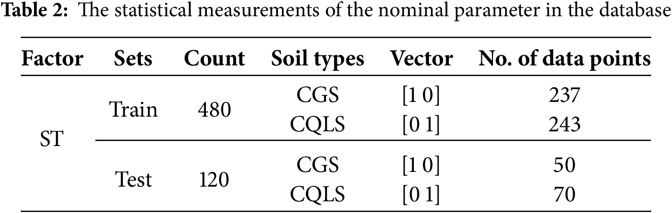
The statistical measurements of numerical and nominal factors in the database, such as minimum, maximum, average, and standard deviation values, are presented in Tables 1 and 2. The soil type variable is categorical. Therefore, the ML models would not misinterpret the data as ordinal with one-hot encoding ordinal logic hierarchies, which is why this format was chosen. In particular, two binary vectors were created to represent the two soil types: CGS was [1 0], and CQLS was encoded as [0 1]. This method was preferred over numerical labels to retain the nominal value of the soil type feature since it avoids unintended implications of ranking or magnitude. The one-hot encoding enabled the models to treat both categories of soil equally, which enhanced model performance and interpretability during the training and evaluation phases.

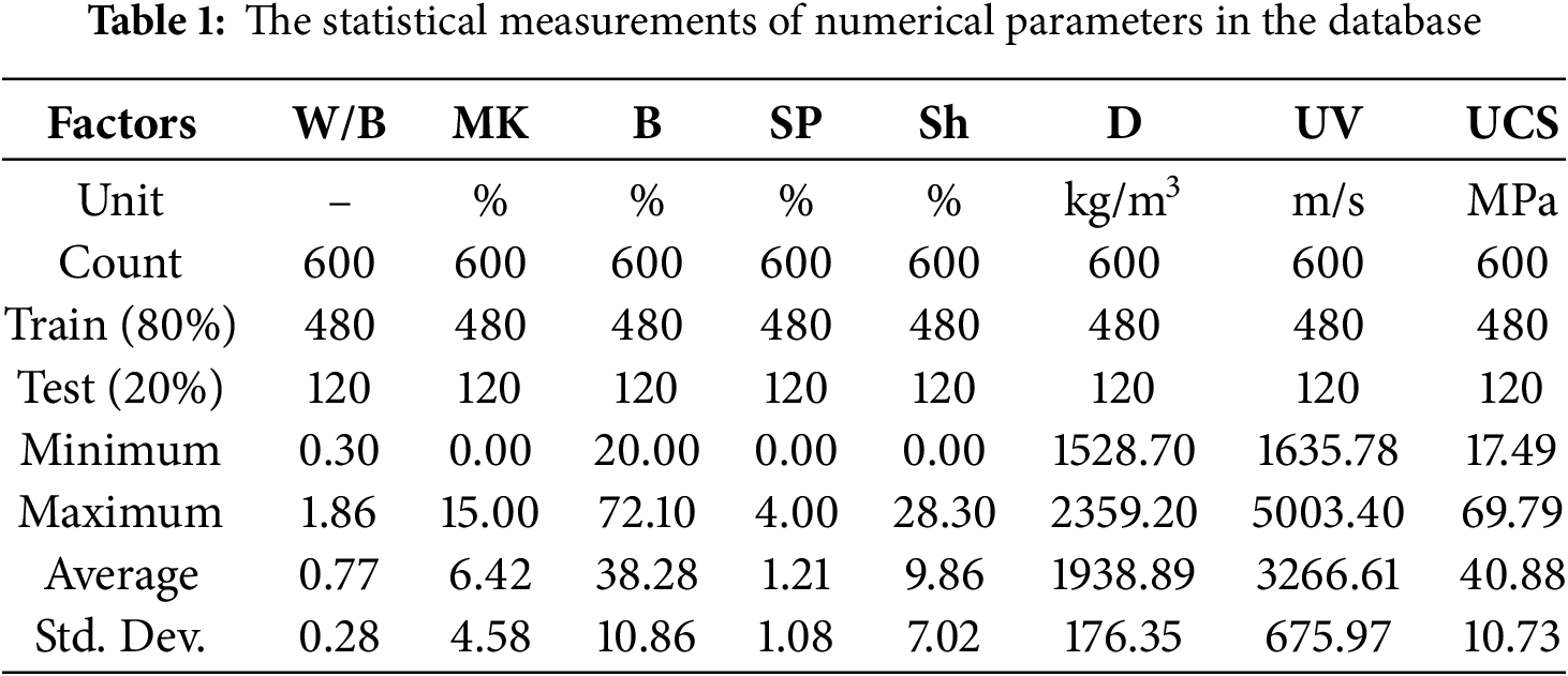
The dataset is made up of 600 samples in total, which were divided into training (n = 480, 80%) and testing (n = 120, 20%) subsets using random stratified sampling. To ensure the robustness and trustworthiness of the ML techniques implemented, special care was made to the equilibrium and partitioning of the dataset. As for the numerical input parameters, their distribution to statistical values is presented in Table 1. The statistical measurements demonstrate a broad and well-dispersed range across all variables, validating that the data set encompasses all conceivable values captured in the laboratory.

The data is pretty evenly distributed, considering the soil type. In the training set, there are 237 CGS samples and 243 CQLS samples. The testing set also has a similar distribution, with 50 CGS and 70 CQLS samples (see Table 2). This distribution allows both soil types to be equally balanced during model training and testing, reducing the chances of model bias towards a specific soil type.

This dataset is essential as it allows the ML models to generalize accurately regardless of the variations in material composition and physical conditions the models are required to work with, increasing the reliability of predictions for soil concrete based on clay or limestone soils.

Fig. 1 presents a boxplot graph for each selected factor, considering their statistical measurements. Fig. 2 also shows the distribution of parameters in the database and their readings for each factor. These graphs show that the generated database has a good distribution of values in both training and testing.

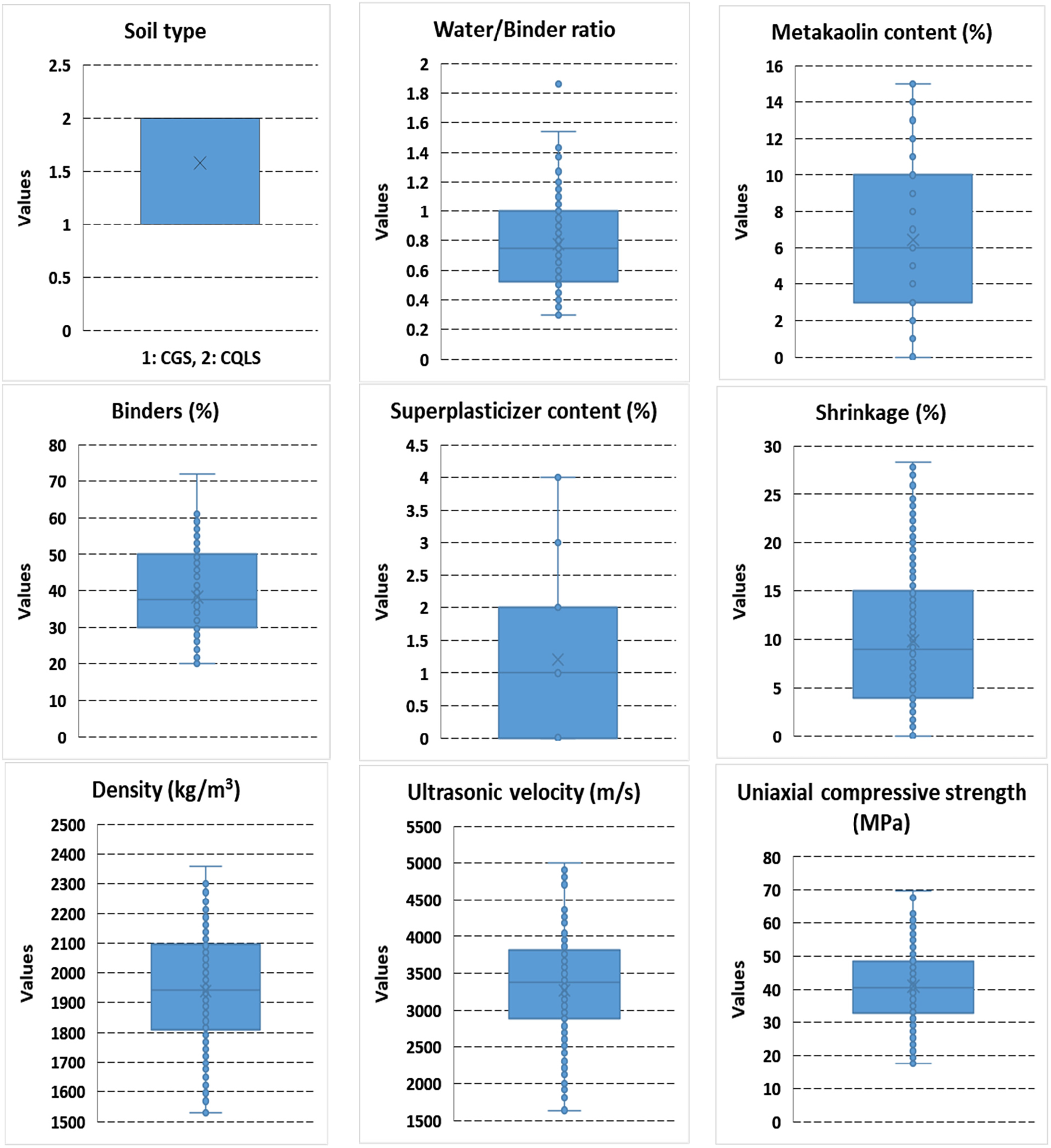
Figure 1: The box plots of input and output parameters for UCS evaluation of soilcrete in this study

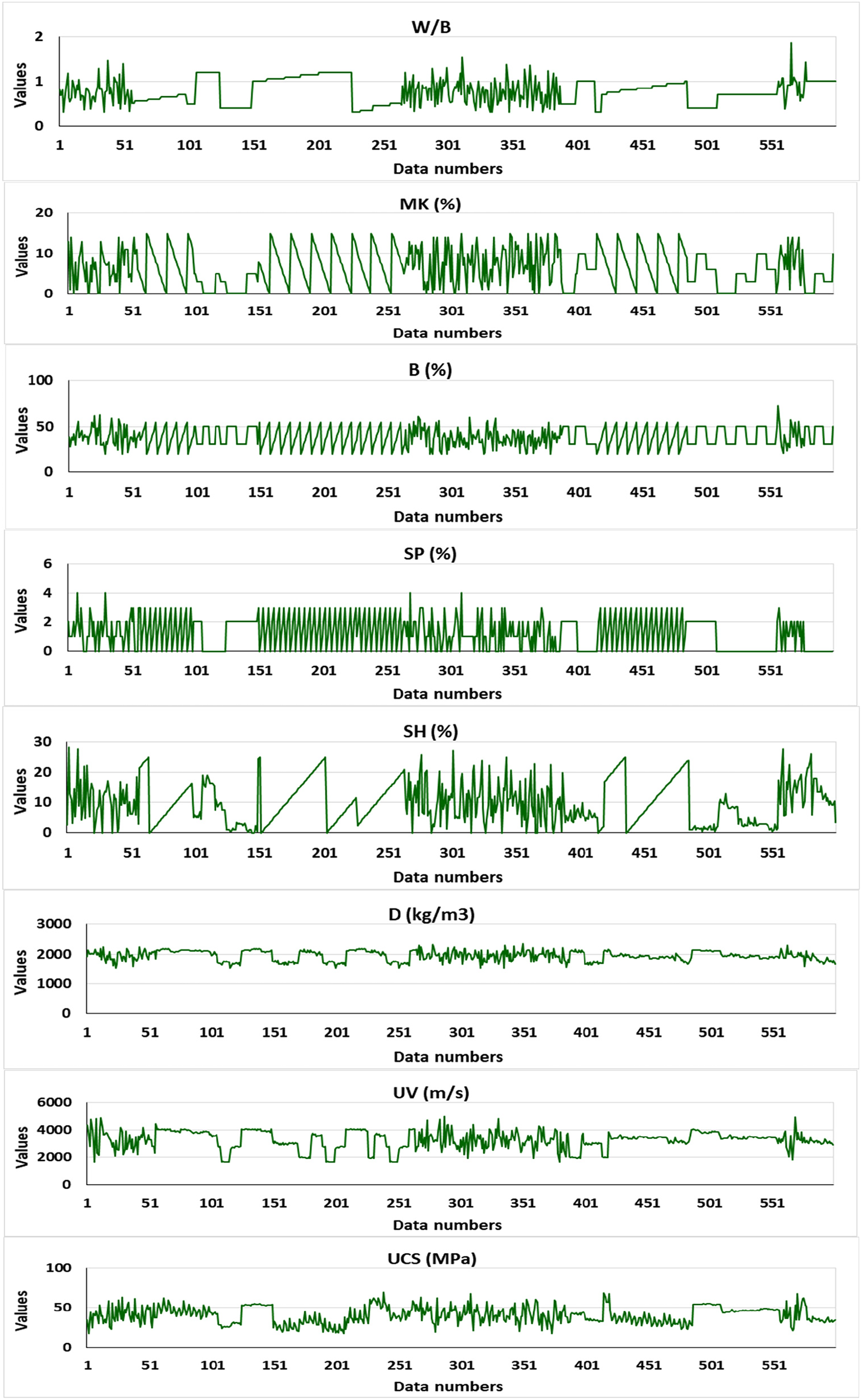
Figure 2: The values of each factor through each reading

Feature engineering is one of the most critical steps in data preprocessing and data processing analysis, where the features and their importance are selected and evaluated for ML investigation. In this article, the extraction method, as one of the most popular techniques used in statistical analysis, was used to consider the influence of each feature from a given dataset and also consider their variance, anti-image covariance, and anti-image correlation. The findings presented in Table 3 show the variance and related measurements utilized principal component analysis (PCA) as one of the extraction methods in two different raw and rescaled tests.

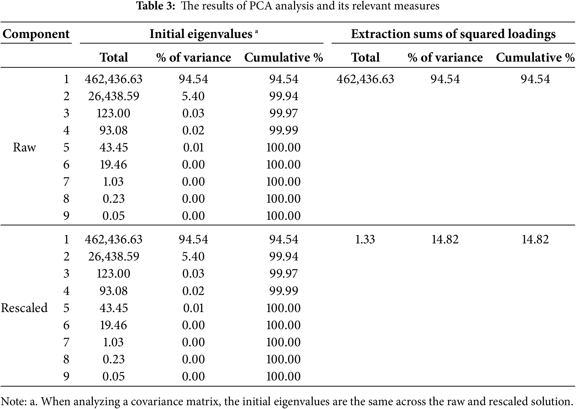
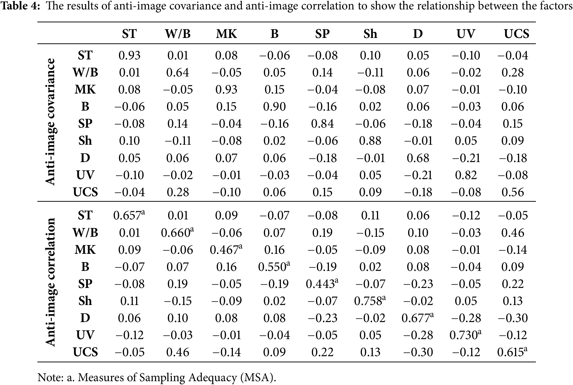
Table 4 presents the anti-image covariance and anti-image correlation for each defined factor in the database. These analyses show the relationship between parameters and also investigate multicollinearity. The values given in this table indicate a low correlation between parameters and the need for the utilization of innovative techniques to identify the patterns and connections between parameters. It is concluded that there is no linear relationship between parameters using simple statistical analysis. Thus, it is necessary to use more advanced functions and ML techniques to find the pattern between factors.

2.3 Data Processing and Normalization

Data normalization is one of the essential steps that should be done before training and testing the ML models to ensure that all readings for all parameters in the database are on the same scale between 0 and 1. After normalization factors in the data processing stage, the parameters were standardized and adjusted in the modeling step with ML techniques. To achieve this standard scale, the StandardScaler method, as one of the data standardization methods, was utilized in this work. Thus, each reading for each parameter was normalized to have a value between zero and one.

Thus, before training the models, as one of the most important preprocessing steps, the database was normalized into 0 to 1 values so that all parameters in the database have a one-scaled configuration without their original units that may differ from each other. The database was collected from laboratory investigations, and so each data point relates to one reading observation in the laboratory analysis. Thus, missing values or duplicated data for each reading in laboratory settings were not presented, as all of the readings were carefully observed for each test.

3  Methodology

3.1 Introduction to Methods

Several ML algorithms, including BPNN, KNN, RBF, FFNN, and SVR, were used for evaluation in the present study. Below is a summarized description of these methods and their justification for the collected database; however, a detailed description of these models can be found in the literature [14–16].

A basic structure within artificial neural networks is the FFNN, which is distinguished by the movement of data in one direction through its layers. In this network, data is processed in a unidirectional manner, starting from the input layer and moving through one or more hidden layers until it reaches the output layer; there are no cycles or feedback loops. In every layer, neurons are connected through weighted connections, which apply activation functions to introduce non-linearity into the model. Because of their structure, FFNNs are capable of modeling very complex patterns within datasets. They are effective in performing regression tasks with intricate and non-linear inter-variable relationships due to their deep learning capabilities. The FFNN was chosen for this study because of its proven effectiveness in capturing intricate input-output mappings and versatility. Its layered structure is particularly well-suited for modeling nonlinear dependencies. These dependencies are typical in geotechnical problems like forecasting the UCS of soilcrete. The FFNN achieves high accuracy because, during training, it modifies its weights according to optimization algorithms, which reduces prediction errors, even when noisy or overlapping input features are used. In this research, the FFNN model presented competitive results and aided in the comparative evaluation of several ML techniques.

SVR seeks to determine a function that best approximates the data within a defined margin of tolerance or a bound. It focuses on a simple model where the regression function is as flat as possible while still allowing a small distance to be off from the actual data points. The best balance SRV provides between accuracy and generalization makes it an easier choice in models for continuous variables, in this case, UCS. SVR was included in the modeling framework due to its capability of solving non-linear regression problems with great accuracy. Its ability to ignore irrelevant noise and generalize from training data fetches predictive models that are both accurate and stable. SVR is particularly beneficial when the dataset sample size is small, which is often the case in soil mechanics and material testing. SVR can provide insights into the elements that determine UCS by adjusting the epsilon margin, penalty parameter (C), kernel function, and other hyperparameters to fit the intricate features of the dataset.

An RBF network is an ANN model that employs radial basis functions (RBFs), usually of the Gaussian type, as activators in one of its hidden layers. They are comprised of three layers: an input layer, a single hidden layer using RBF units, and an output layer. RBF networks are renowned for their speed in training and their capability to approximate functions, especially for highly non-linear and local problems with a steep relationship between the input and output. RBF was used in this work because of its effectiveness in modeling localized patterns and its quick response to intricate data structures. RBF networks have a less complex architecture and achieve faster convergence than deeper neural architectures while maintaining high accuracy in prediction tasks. Concerning predicting UCS of soilcrete, the RBF model indicated excellent performance, which shows its effectiveness in solving problems where processes act on variables, such as binder composition, moisture content, and density, through local interactions. The addition of the RBF model offered a compelling comparison to other neural network-based models in terms of performance and efficiency.

KNN operates on a similarity principle by predicting the outcome based on the ‘K’ closest neighbors in feature space. Standard proximity measures include distance metrics like Euclidean distance. KNN is unique as it requires no explicit training phase apart from storing the training dataset. KNN’s simplicity and transparency make it particularly effective when the data distribution is unknown or irregular. Within automated laboratory-based studies like this one, wherein the model input conditions are often highly constrained due to arbitrary factors, KNN remains a robust benchmark model. Moreover, KNN’s lack of rigid assumptions enables it to capture intricate relationships. Additionally, its effectiveness in accommodating nonlinear relationships and mixed data types makes KNN well-suited for the heterogeneous and diverse soilcrete dataset used in this study.

A supervised, multilayer feedforward neural network trained with the backpropagation algorithm is called BPNN. The output is made up of subclasses that are physically present in the input. It works by having a delay element and filters. During training, the predicted output and the expected output of the model are compared to assess performance, and the result computed is propagated backward through the network to adjust weights using gradient descent. Model training continues until a defined objective is reached. BPNNs are capable of solving complex regression problems due to their flexibility and ability to approximate a wide range of functions. The reason BPNN was selected in this study is its ability to model complex relationships that are non-linear between the input features and target outputs.

It should be mentioned that the gradient descent (GD) optimization technique is directly used for BPNN and FFNN neural networks to optimize their outcomes in both the training and testing phases. For other used algorithms in this study, it should be mentioned that KNN is a non-parametric, instance-based learning algorithm and does not inherently involve a training phase or optimization of a cost function via gradient descent, as in models like BPNN and FFNN. In this study, gradient descent was not used to optimize the KNN algorithm itself directly but instead to fine-tune its hyperparameters—like the number of neighbors (k) and how distances are weighted—by minimizing a loss function and evaluation metrics using performance metrics. Also, for SVR and RBF models, the GD technique was utilized for hyperparameters for models directly for RBF and indirectly for SVR. This approach involved treating the hyperparameter selection as an optimization problem, where gradient-based techniques were applied over a continuous approximation of the hyperparameter space. In the present study, we used different optimization techniques such as gradient descent, scaled conjugate gradient, Adam, AdaDelta, etc., to improve the results and make hybrid models. However, based on the results of loss functions and evaluation metrics, we observed that gradient descent showed better results than others for this database.

To determine the best hyperparameters and their optimal range for each model, a range of values that seemed reasonable based on previous studies, engineering judgment, commonly used practices, and the gradient descent technique was applied. The algorithms were trained several times using different combinations within those ranges. Throughout this process, we evaluated how well each model performed by looking at prediction accuracy and key metrics like loss functions and evaluation metrics. By comparing the results across these runs, the set of hyperparameters that gave the most reliable and accurate outcomes was determined. These chosen values, along with the optimal ranges, were presented in Table 5.

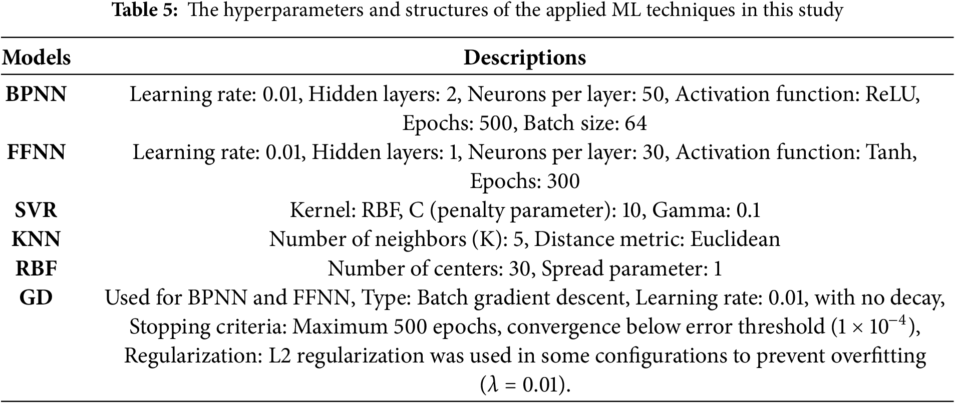
In this study, hyperparameter tuning was conducted manually through a series of iterative experiments. Based on prior knowledge, literature, and engineering judgment, a reasonable range of values for the key hyperparameters was provided for each ML model. The model’s performance under different combinations within those ranges was evaluated. The tuning process involved systematically adjusting one or more hyperparameters at a time, observing the resulting changes in performance metrics, and selecting the combination that yielded the most accurate predictions on the test dataset.

Although methods like grid search or cross-validation were not used, the manual tuning approach (manual tuning based on iterative testing), repeated across multiple iterations, allowed us to identify optimal configurations that balanced model accuracy and generalizability effectively. This way worked better for this database, as in the current study, the number of hyperparameters was manageable, and based on laboratory investigations, a knowledge of the best distribution existed to initial choices, as well as the good observations of performing the models through each tuning.

A fixed train-test split was used as a validation technique, ensuring that the data used for model evaluation was entirely independent of the data used for training. The dataset was randomly split into training and testing sets (70/30, 80/20, 85/15 split) within SPSS software using the Select Cases and Split File functions. In addition, residual analysis was used as a model validation technique.

3.2 Computational Cost and Scalability

Among the models applied, BPNN and FFNN typically require more computational resources during training due to iterative optimization and parameter tuning, especially with larger datasets. However, once trained, their prediction times are fast and stable, making them suitable for real-time applications. SVR is efficient for small- to medium-sized datasets, which aligns well with typical datasets in geotechnical studies involving soilcrete (in the current study, 600 data points with eight features). KNN requires minimal training time but has higher prediction-time complexity, which may limit its scalability unless optimized with indexing techniques such as KD-trees [15].

3.3 Feasibility of Deployment in Engineering Workflows

In the context of UCS prediction for soilcrete, models like FFNN, BPNN, and SVR are particularly suitable for engineering design tools and geotechnical software. These models can be trained offline and embedded in computer-aided design (CAD) environments, or used as backend modules in real-time monitoring systems for deep mixing or soil stabilization projects. Their rapid inference capability and ease of deployment through modern ML libraries (e.g., TensorFlow Lite, ONNX) enhance their practical usability. While KNN and RBF networks also show strong predictive ability, they may require additional optimization for use in time-sensitive or large-scale applications.

4  Results and Discussions

4.1 Simple Regression-Based Analysis

This section of the paper presents the results of multivariable regression analysis. Before using ML techniques, the new empirical model was developed based on the multivariable regression technique. In this technique, all of the input parameters were considered as independent variables and the output factor was considered as a dependent variable. In this technique, based on stepwise analysis, it was concluded that all of the defined parameters (ST, W/B, B, MK, B, SP, Sh, D, UV, UCS) should be considered for developing an empirical model. The developed formula is presented in Eq. (1). Each factor in this model has a specific weight based on its influence (high or low impact) on the output factor (UCS), which was determined in the analysis process using stepwise multivariable analysis. The high unstandardized coefficients indicate the high influence of the input factor on the output, and the low value of this coefficient means a lower impact on the output.

UCS=19.869+0.923ST−16.574W/B+0.253MK−0.068B−1.786SP−0.158Sh+0.017D+0.002UV(1)

For evaluating the accuracy and precision rate of this formula, several statistical metrics, including R, R2, adjusted R2, standard error of the estimate, change statistics, and the Durbin-Watson test, were considered for investigation. The results of these metrics are presented in Table 6. Also, the results of the analysis of variance (ANOVA), including several metrics for regression, residual, and total for this formula, are presented in Table 7. The correlation between measured-actual values in laboratory settings and calculated results from this empirical model is presented in Fig. 3. Based on the results in the tables and figure, it is concluded that the developed empirical formulas based on multi-variable regression analysis do not have a high accuracy rate in the estimation of UCS of soilcrete with R2 = 0.43 and standard error of the estimate rate = 8.12. Thus, there is a need to add more investigation using more advanced models based on ML algorithms to find the pattern between parameters and achieve a higher accuracy rate in prediction.

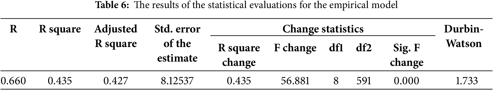
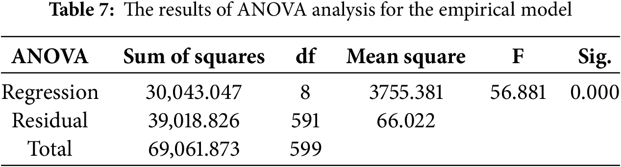
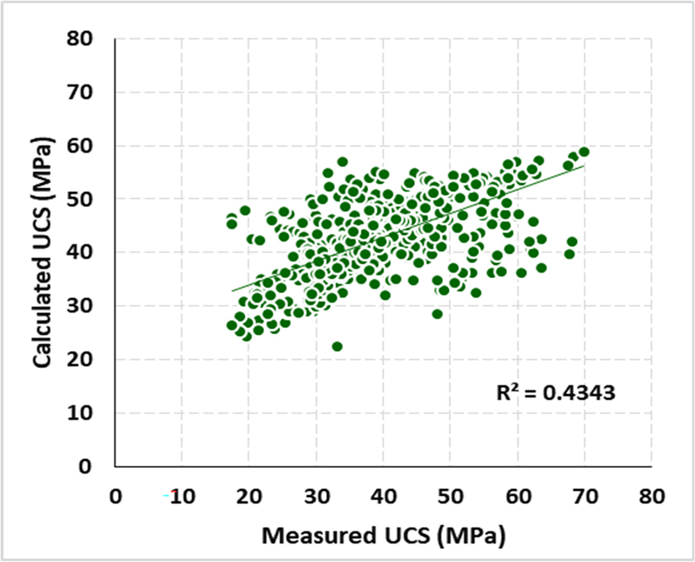
Figure 3: The correlation between measured (laboratory) and calculated (empirical model) values for UCS

A tornado graph-sensitivity analysis based on the developed empirical model was done. The tornado diagrams corresponding to the proposed multivariable regression models for UCS of soilcrete are presented in Fig. 4. As shown, three parameters, including UV, D, and B, have the least impact on UCS. However, the W/B and SP are critical parameters affecting the UCS.

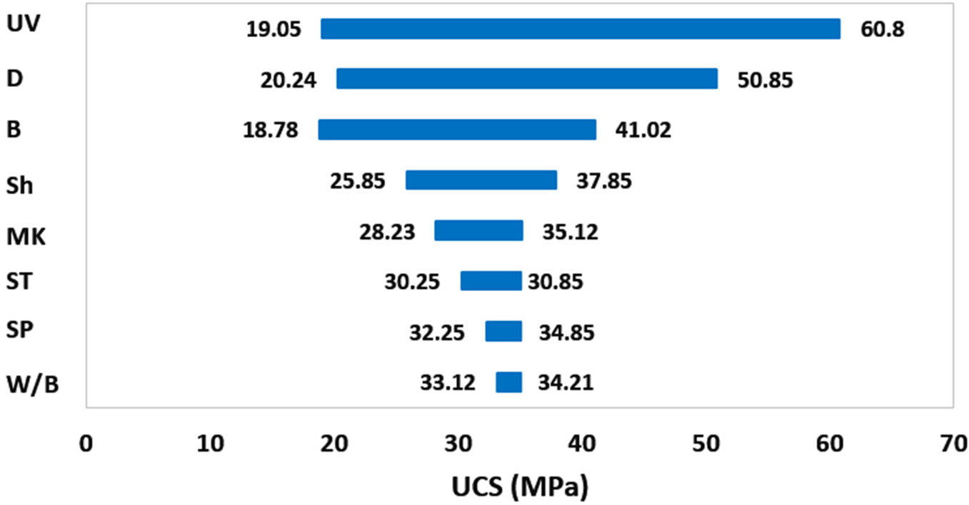
Figure 4: Sensitivity analysis based on an empirical equation

4.2 Machine Learning Investigtions

In this study, several ML algorithms, including back-propagation neural network (BPNN), K-nearest neighbor (KNN), radial basis function (RBF), support vector regression (SVR), and feed-forward neural network (FFNN), were utilized for prediction. All of these algorithms were optimized using one of the optimization techniques, namely gradient descent (GD). 80% of the data points were used for training and 20% were used for testing the models. The results of ML algorithms and their comparison with measured values in laboratory settings are presented in Fig. 5.

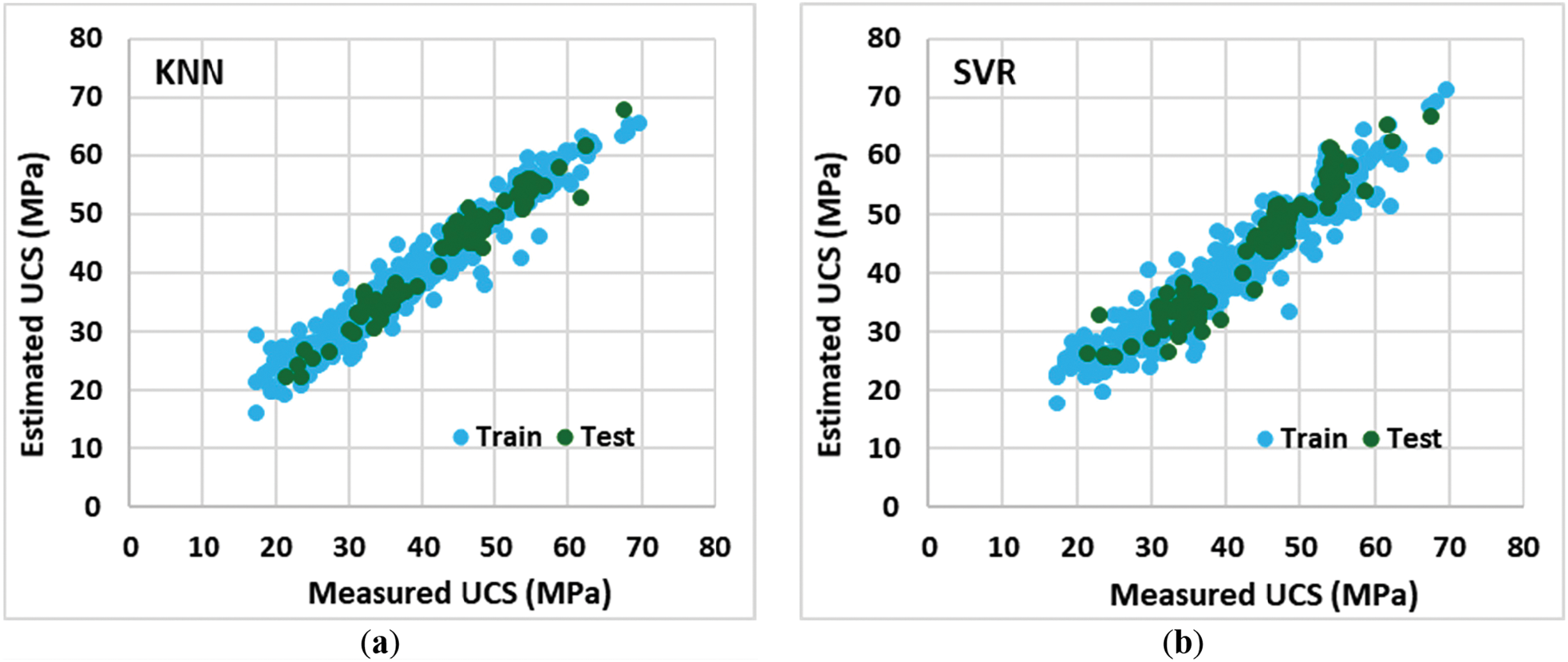
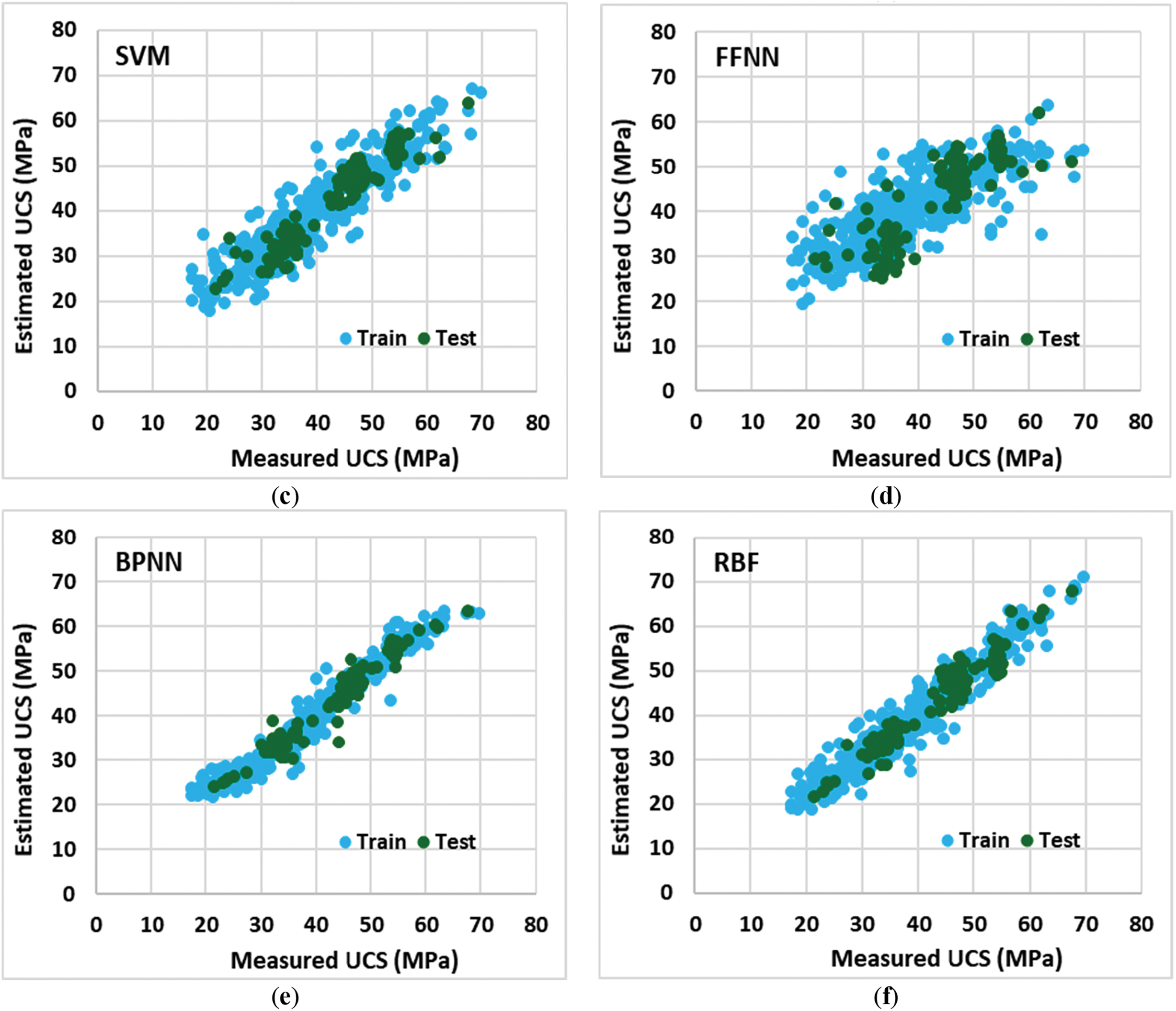
Figure 5: The correlation between the predicted and measured values of UCS using laboratory and ML analysis. (a) KNN; (b) SVR; (c) SVM; (d) FFNN; (e) BPNN; (f) RBF

For the evaluation accuracy of each model in prediction, several evaluation metrics and loss functions were used. The utilized evaluation metrics in this study are root mean square error (RMSE), mean absolute percentage error (MAPE), relative absolute error (RAE), and median absolute deviation (MAD). The formulas of these metrics were presented in Eqs. (2)–(5), where “P” is the predicted values, “A” is the actual values, and “n” is the number of data points. The results of these metrics for each ML algorithm are presented in Table 8. Based on the presented results in Table 8, it is concluded that all of the algorithms show acceptable performance in both training and testing as the values of these metrics approach zero, and also the value of R2 approaches one. The results of these metrics for training and testing separately are presented in Figs. 6 and 7.

RMSE=∑i=1n(P−A)2n(2)

MAD=∑|P−average(P)|n(3)

MAPE=1n∑|A−PA|(4)

RAE=∑i=1n|A−P|∑i=1n|A−average(A)|(5)

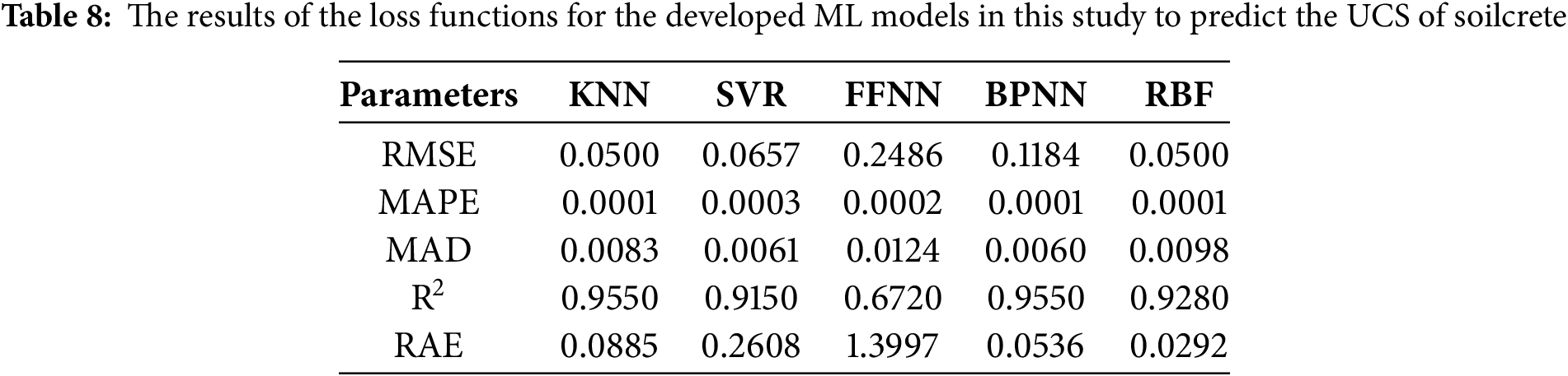
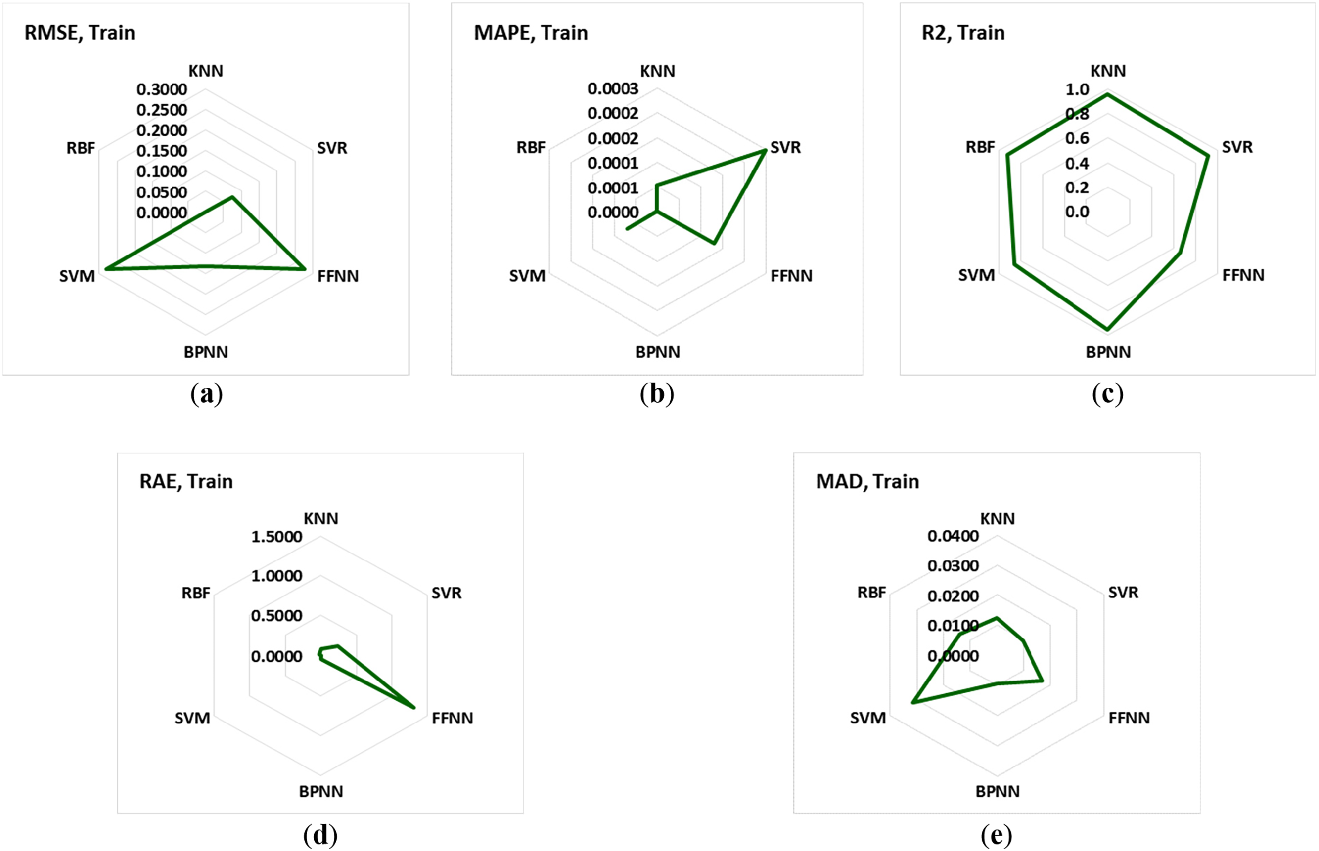
Figure 6: The results of the evaluation metrics for the training dataset of each model. (a) RMSE; (b) MAPE; (c) R2; (d) RAE; (e) MAD

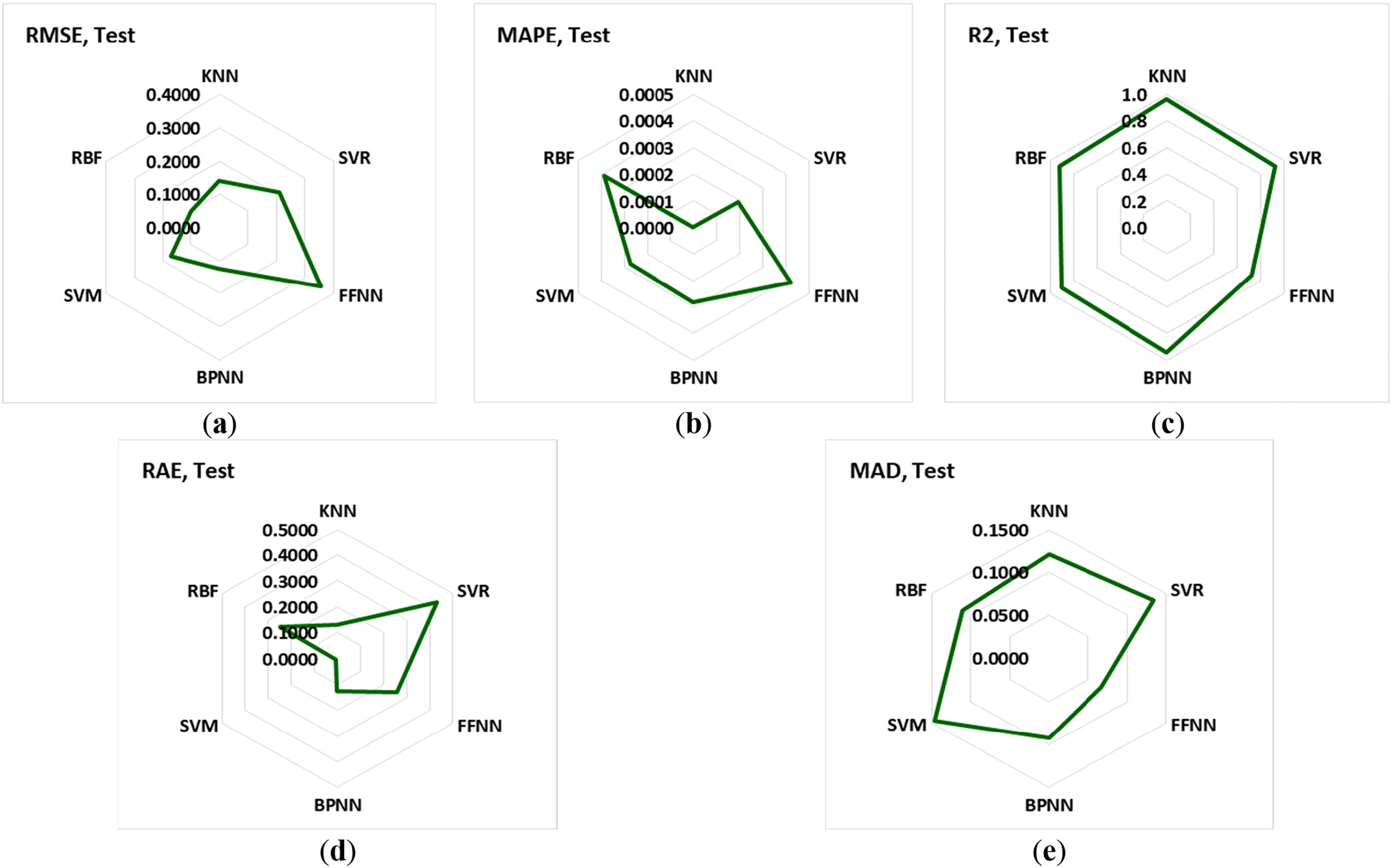
Figure 7: The results of the evaluation metrics for the testing dataset of each model. (a) RMSE; (b) MAPE; (c) R2; (d) RAE; (e) MAD

Table 9 indicates the score value (1–6; because of the number of models) for each evaluation metric (RMSE, MAPE, MAD, RAE, R2) for ML algorithms. The lowest values for RMSE, MAPE, MAD, and RAE metrics have the highest score (n = 6); however, for R2, the highest value of this metric has the highest score (n = 6). This is because the lower values of loss functions and higher values of R2 show more accuracy and reliability in prediction. It should be noted that, when the value of a metric is the same for two models, both models receive the same score, and this time the maximum score is reduced from 6 to 5. Fig. 8 indicates the total score for each model using the ranking score of each evaluation metric, which is presented in Table 9. This analysis shows that the BPNN has more accuracy and reliability in prediction than the other models, with a total score ranking of 21. RBF and KNN have more accuracy compared to the other models, with a ranking score of 18. However, FFNN has lower accuracy than the other models, with a score ranking of 6. SVR has a score ranking of 12.

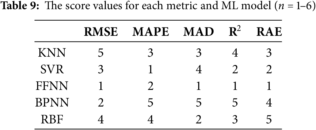
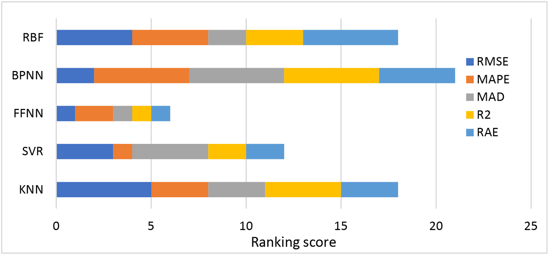
Figure 8: Comparison between the performance of ML models based on their ranking score analysis

To monitor and prevent overfitting, model performance using evaluation metrics on the test dataset was assessed. The stable performance across training and test sets indicated that no signs of overfitting were present in the analysis. By comparing the MSE and R2 values presented in the study, there was no extended difference between them, which proved that the model generalized well.

In addition to these analyses, for further evaluation, the outcomes of models and their accuracies were measured using statistical metrics such as the Durbin-Watson test, change statistics, and other statistical measurements. The results of these analyses are summarized in Table 10. As can be seen, the models show acceptable performance in prediction. Also, Fig. 9 presents the results of the distribution of relative error rates in both training and testing. These histograms indicate not only the acceptable range of error rate in prediction but also a high accuracy rate for all applied models.

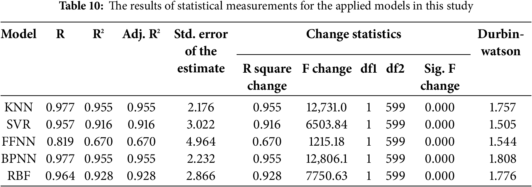
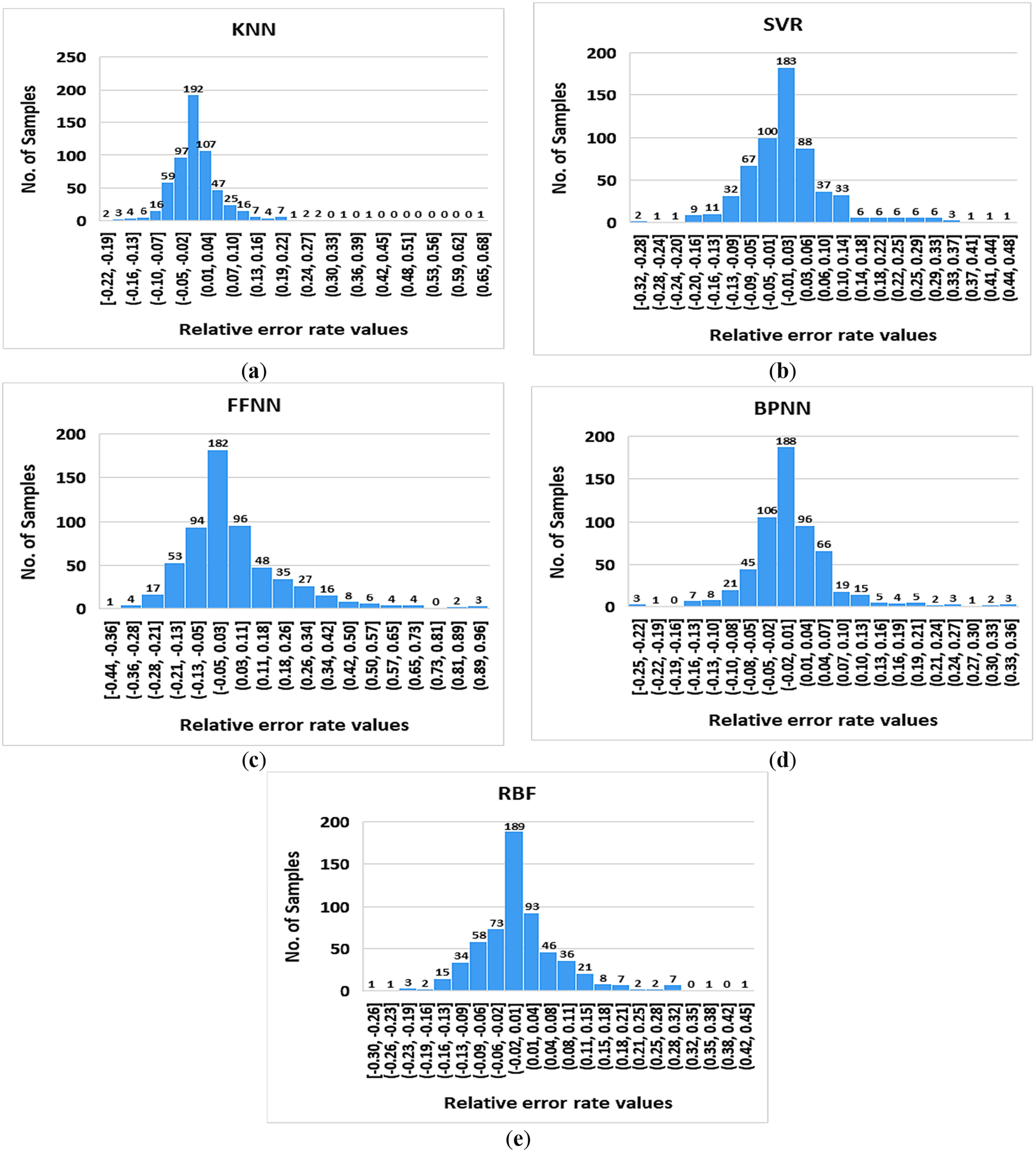
Figure 9: The histograms of relative error rate in prediction based on the results of the applied ML models in this study, (a) KNN; (b) SVR; (c) FFNN; (d) BPNN; (e) RBF

Fig. 10 presents the plots of frequency vs. regression standardized residuals for all applied ML techniques. The histogram of standardized residuals should indicate a bell-shaped curve, as deviation from normality indicates misspecification in the models or the presence of outliers. The best performance of models should show residuals centered around zero without skewness. As can be seen, all of the models show a bell-shaped curve with normal distribution and residuals centered around zero, which proves not only the high accuracy rate of models in prediction, but also the absence of misspecification in the models and outliers.

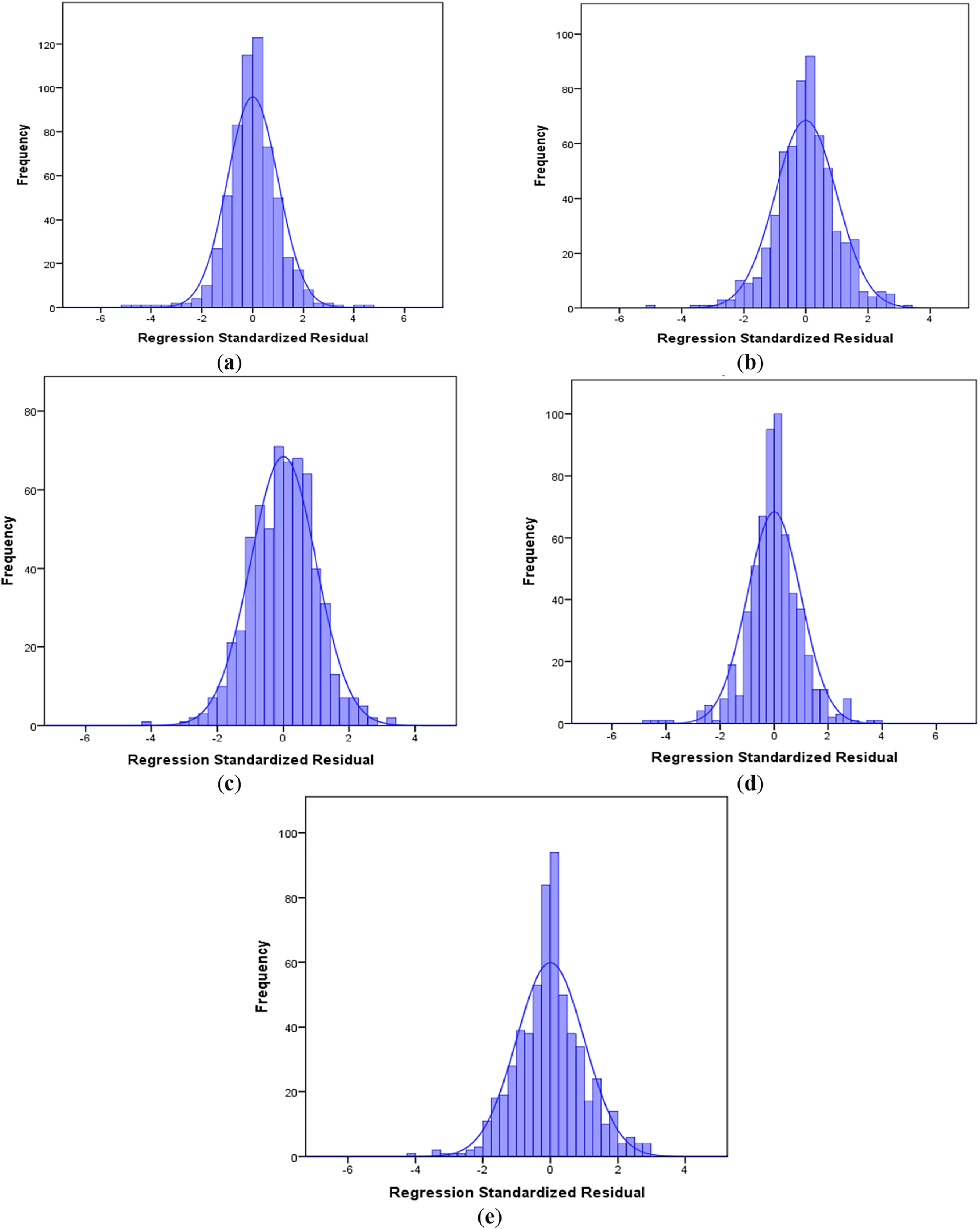
Figure 10: The plots of frequency vs. regression standardized residuals for applied ML techniques. (a) KNN, (b) SVR, (c) FFNN, (d) BPNN, (e) RBF

Each input factor has a specific impact and importance on the prediction performance. Some factors have higher importance on the results of prediction, and some others have a lower impact. The influence of each input parameter on the result of the prediction can be obtained using importance ranking analysis. Thus, the sensitivity analysis in this study was conducted based on feature importance analysis derived directly from the internal mechanics of the ML models. Specifically, the feature importance measures provided by the algorithms used, such as weights, coefficients, and split importance, depending on the nature of each model, were utilized. This approach evaluated the relative contribution of each input variable to the model’s predictions. The results of this importance ranking are presented in Fig. 11 for each technique. As can be seen, W/B, UV, B, and D have more important values than others in all models; however, specifically, in the RBF model, W/D and MK have a higher impact on the ML results compared to others. BPNN shows that, in addition to the W/B factor, another factor, namely D, has a high impact on the prediction results. In the KNN model, parameters B and D have a higher impact compared to the others. However, in the FFNN model, the other two factors, including D and SP, show more influence. The SVR model shows that the UV factor has a higher influence than other parameters.

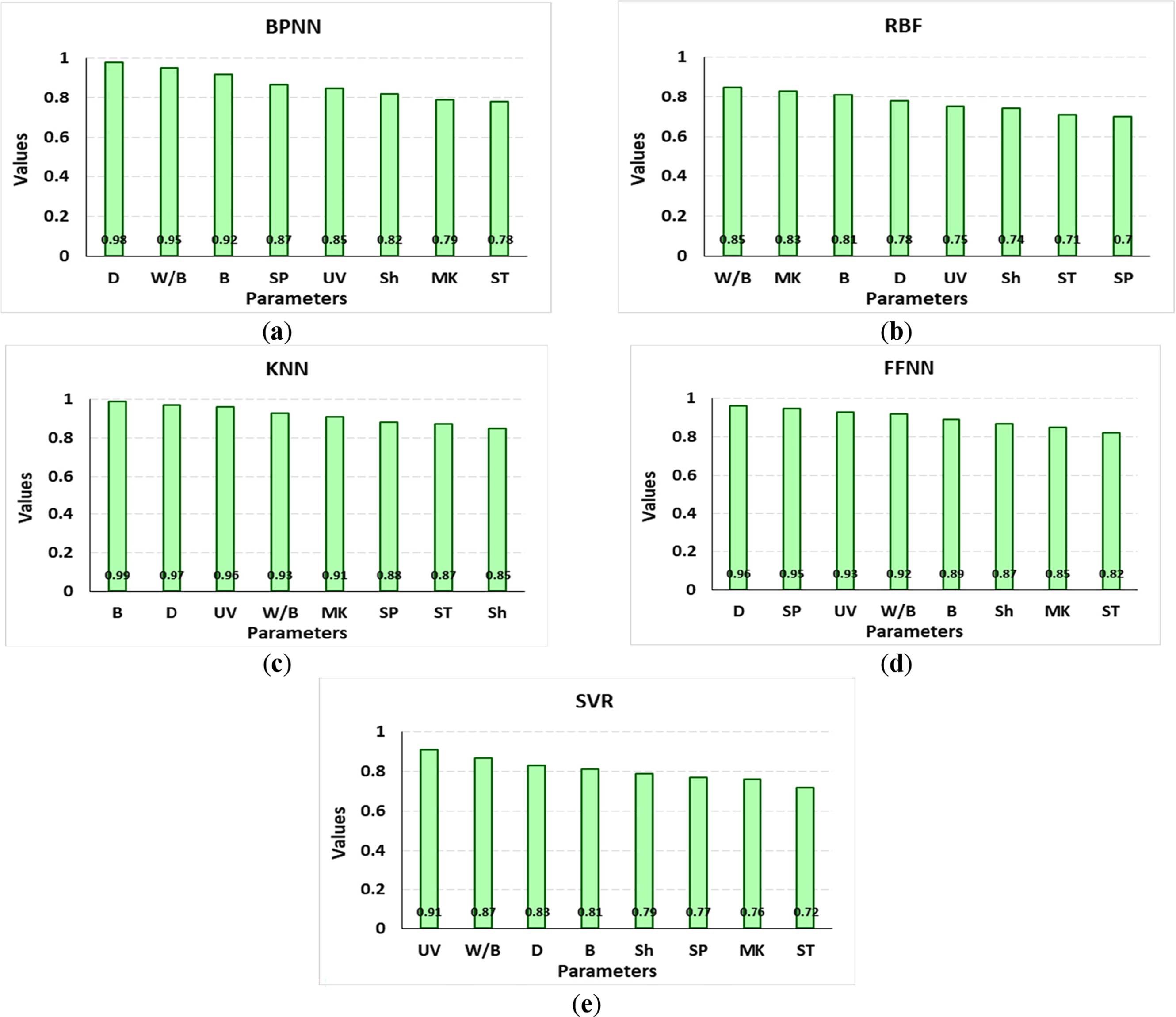
Figure 11: The results of importance ranking based on the outcomes of ML techniques. (a) BPNN; (b) RBF; (c) KNN; (d) FFNN; (e) SVR

5  Future Directions of This Study

An emerging and promising area in ML for materials science is the application of Physics-Informed Neural Networks (PINNs). These models integrate known physical laws (such as differential equations, boundary conditions, and conservation principles) directly into the training process of neural networks. This hybrid modeling framework allows PINNs to not only learn from data but also adhere to governing physical laws. This improves generalizability and robustness, especially when experimental data is sparse or noisy. Incorporating PINNs in future studies could enhance the interpretability and physical consistency of UCS predictions, especially in soilcrete systems where the mechanical behavior stems from complex interactions between soil particles, binders, moisture, and particulate dynamics.

Moreover, the blending of physical constitutive equations from classical soil mechanics and material science offers an intriguing potential area of research. Such constitutive models can be employed as constraints or regularization factors in data-driven implementations, for example, models based on stress-strain relationships or the theories of poromechanics. From a solver-centric approach, coupling some of these constitutive relations with numerical procedures, such as finite element models, augurs well for ML. This will allow hybrid models where mechanistic simulations are complemented with data-driven predictions to be optimized through ML. Enhanced integration would improve the quantification of UCS and other geotechnical parameters while ensuring that the predictions are physically rather than verifiably grounded.

These approaches develop the opportunity to curate sophisticated empirical datasets through interpretable algorithms while satisfying the principles of physics operating in composite geomaterials, like soil concrete, not just through soil mechanics laws. Such physics-informed approaches are essential as the field matures to close the gap between meaningfully actionable insights and black-box predictions.

6  Conclusions

This research analyzed the application of specific ML algorithms to estimating the UCS of soilcrete. A laboratory-based dataset containing 600 data points along with a comprehensive set of associated geotechnical, physical, and soil-type conditions was created. In total, 80% of that dataset was used to train the ML models, and the remaining 20% was kept for validation purposes. Using multivariable regression, an empirical equation predicting UCS was developed with a standard error of 8.12. Several ML models were also applied and assessed alongside that baseline for comparison, including RBF, KNN, BPNN, SVR, and FFNN. Direct gradient descent optimization was performed on the neural network models, while all other models were tuned via hyperparameter optimization. Various loss functions were implemented to assess accuracy, robustness, and overall model evaluation.

The analysis provided insight into how each model performed and noted that all models attained acceptable accuracy benchmarks. Overall, the BPNN model performed best with the highest accuracy (ranking score = 25), while the least effective was the FFNN model (ranking score = 7). The order of the models in terms of prediction accuracy was: BPNN, RBF, KNN, SVR, and FFNN. Further sensitivity analysis demonstrated that all ML model input parameters were important in predicting performance. In particular, parameters W/B ratio, UV, B, and D emerged as the most influential parameters for the majority of the models.

Even with its potential benefits, this study points out the lack of work done on the ML-based forecasting of property soilcrete’s mechanical features and indicates one gap that is yet to be filled in the field. Additional experimental work should focus on broadening the dataset by integrating more soilcrete physical and mechanical attributes, expanding the range of soilcrete characteristics, and augmenting soilcrete features. Furthermore, the application of different ML and deep learning techniques and their optimizations could increase the accuracy of predictions. While this study concentrated on two types of soil, other types with various additives, curing times, and W/B ratios should be examined for model applicability and usefulness.

Acknowledgement: The authors would like to acknowledge the support of Prince Sultan University for paying the Article Processing Charge (APC) of this publication and their support. Princess Nourah bint Abdulrahman University Researchers Supporting Project number (PNURSP2025R300).

Funding Statement: The support of Prince Sultan University for paying the Article Processing Charge (APC) of this publication and their support. Princess Nourah bint Abdulrahman University Researchers Supporting Project number (PNURSP2025R300).

Author Contributions: The authors confirm contribution to the paper as follows: Conceptualization, Ala’a R. Al-Shamasneh and Faten Khalid Karim; methodology, Arsalan Mahmoodzadeh; software, Arsalan Mahmoodzadeh; validation, Ala’a R. Al-Shamasneh, Faten Khalid Karim, and Arsalan Mahmoodzadeh; formal analysis, Arsalan Mahmoodzadeh; investigation, Arsalan Mahmoodzadeh; resources, Arsalan Mahmoodzadeh; data curation, Arsalan Mahmoodzadeh; writing—original draft preparation, Arsalan Mahmoodzadeh; writing—review and editing, Arsalan Mahmoodzadeh; visualization, Arsalan Mahmoodzadeh; supervision, Ala’a R. Al-Shamasneh; project administration, Ala’a R. Al-Shamasneh; funding acquisition, Ala’a R. Al-Shamasneh. All authors reviewed the results and approved the final version of the manuscript.

Availability of Data and Materials: Data not available due to restrictions imposed by research sponsors, ongoing analysis for future studies, and the necessity to maintain data confidentiality until further validation and publication.

Ethics Approval: Not applicable.

Conflicts of Interest: The authors declare no conflicts of interest to report regarding the present study.

References

1. Kolovos KG, Asteris PG, Cotsovos DM, Badogiannis E, Tsivilis S. Mechanical properties of soilcrete mixtures modified with metakaolin. Constr Build Mater. 2013;47:1026–36. doi:10.1016/j.conbuildmat.2013.06.008. [Google Scholar] [CrossRef]

2. Emad W, Salih A, Kurda R. Stress-stain behavior, elastic modulus, and toughness of the soilcrete modified with powder polymers. Constr Build Mater. 2021;295:123621. doi:10.1016/j.conbuildmat.2021.123621. [Google Scholar] [CrossRef]

3. Helson O, Beaucour AL, Eslami J, Noumowe A, Gotteland P. Physical and mechanical properties of soilcrete mixtures: soil clay content and formulation parameters. Constr Build Mater. 2017;131:775–83. doi:10.1016/j.conbuildmat.2016.11.021. [Google Scholar] [CrossRef]

4. Mazhnik E, Oganov AR. Application of machine learning methods for predicting new superhard materials. J Appl Phys. 2020;128(7):075102. doi:10.1063/5.0012055. [Google Scholar] [CrossRef]

5. Bagher Shemirani A. Prediction of fracture toughness of concrete using the machine learning approach. Theor Appl Fract Mech. 2024;134:104749. doi:10.1016/j.tafmec.2024.104749. [Google Scholar] [CrossRef]

6. Alipour M, Esatyana E, Sakhaee-Pour A, Sadooni FN, Al-Kuwari HA. Characterizing fracture toughness using machine learning. J Pet Sci Eng. 2021;200:108202. doi:10.1016/j.petrol.2020.108202. [Google Scholar] [CrossRef]

7. Tarawneh A, Saleh E, Almasabha G, Alghossoon A. Hybrid data-driven machine learning framework for determining prestressed concrete losses. Arab J Sci Eng. 2023;48(10):13179–93. doi:10.1007/s13369-023-07714-y. [Google Scholar] [CrossRef]

8. Bin Inqiad W, Javed MF, Siddique MS, Alarifi SS, Alabduljabbar H. A comparative analysis of boosting and genetic programming techniques for predicting mechanical properties of soilcrete materials. Mater Today Commun. 2024;40:109920. doi:10.1016/j.mtcomm.2024.109920. [Google Scholar] [CrossRef]

9. Ala’a R, Mahmoodzadeh A, Ghazouani N, El Ouni MH. Forecasting mechanical properties of soilcrete enhanced with metakaolin employing diverse machine learning algorithms. Geomech Eng. 2025;40(2):123–37. doi:10.12989/gae.2025.40.2.123. [Google Scholar] [CrossRef]

10. Inqiad WB, Khan MS, Mehmood Z, Khan NM, Bilal M, Sazid M, et al. Utilizing contemporary machine learning techniques for determining soilcrete properties. Earth Sci Inform. 2025;18(1):176. doi:10.1007/s12145-024-01520-2. [Google Scholar] [CrossRef]

11. Hemdan EED, Al-Atroush ME. An efficient IoT-based soil image recognition system using hybrid deep learning for smart geotechnical and geological engineering applications. Multimed Tools Appl. 2024;83(25):66591–612. doi:10.1007/s11042-024-18230-y. [Google Scholar] [CrossRef]

12. Sun Y, Li G, Zhang J. Developing hybrid machine learning models for estimating the unconfined compressive strength of jet grouting composite: a comparative study. Appl Sci. 2020;10(5):1612. doi:10.3390/app10051612. [Google Scholar] [CrossRef]

13. Asteris PG, Alexandridis A, Kolovos KG, Anesti EG, Douvika MG, Karamani CA, et al. Prediction of mechanical characteristics of soilcrete materials using artificial neural networks. In: 7th International Conference on Mechanics and Materials in Design; 2017 Jun 11–15; Albufeira, Portugal. [Google Scholar]

14. Abdolrasol MG, Hussain SS, Ustun TS, Sarker MR, Hannan MA, Mohamed R, et al. Artificial neural networks based optimization techniques: a review. Electronics. 2021;10(21):2689. doi:10.3390/electronics10212689. [Google Scholar] [CrossRef]

15. Cunningham P, Delany SJ. K-nearest neighbour classifiers-a tutorial. ACM Comput Surv. 2021;54(6):1–25. doi:10.1145/3459665. [Google Scholar] [CrossRef]

16. Khan AA, Laghari AA, Awan SA. Machine learning in computer vision: a review. EAI Endorsed Trans Scalable Inf Syst. 2021;8(32):1–11. doi:10.4108/eai.21-4-2021.169418. [Google Scholar] [CrossRef]