Behavior of Spikes in Spiking Neural Network (SNN) Model with Bernoulli for Plant Disease on Leaves

1  Introduction

Spiking Neural Networks (SNNs) simulate the behavior of natural neurons by producing sudden, short voltage spikes to transfer information between sending and receiving neurons. In biological systems, these brief electrical impulses, known as spikes or pulses, facilitate communication within the nervous system [1]. SNNs are considered the third generation of Artificial Neural Networks (ANNs) [2]. Traditional ANNs, commonly used in digital image processing, often lack features such as synaptic plasticity and require extensive pre-processing and tuning, which vary widely between applications [3–5]. While traditional techniques such as CNNs and FCNNs have been widely applied in plant disease detection, they typically process static images and thus overlook the temporal dynamics that are critical for early disease identification. In contrast, SNNs exploit time-dependent, event-driven spikes that capture both spatial and temporal features, offering a more robust and energy-efficient approach.

Moreover, our approach incorporates Bernoulli trials early in the processing pipeline to regulate spike generation. This mechanism selectively activates neurons only when relevant features are present, significantly reducing unnecessary neural activity and computational overhead, a key advantage for real-time, resource-constrained agricultural applications. Neuromorphic computing aims to replicate brain functions, representing the future direction of AI [6]. Plant diseases have a significant impact on crop yield by adversely affecting plant growth and reproduction. Contaminated plant leaves can severely reduce crop production, requiring early detection and proactive measures to mitigate the effects [7]. Early disease detection through neural networks and machine learning enables timely preventive actions, addressing crop diseases and food insecurity affecting millions globally [8,9]. The design of artificial neural networks draws inspiration from biological neurons, which receive signals from the body and relay them to the brain. These neurons, with specialized cell structures, can generate electrical or chemical signals that are transmitted to other connected neurons [10].

Despite variations in their shapes and sizes depending on their location in the body, they share common structural features such as axons, dendrites, and cell bodies [11]. Biological neurons also contain synapses that have action potential [12]. In artificial neurons, input signals consist of numeric arrays rather than biological electrical pulses [13]. The research paper investigates the characteristics and behaviors of Spiking Neural Networks (SNNs), the third generation of artificial neural networks (ANNs), which operate similarly to biological neural networks by processing information in the form of spikes concerning time [14]. Unlike traditional ANN models, SNNs are designed to mimic spike-based communication within biological neurons, as shown in Fig. 1, offering a more biologically realistic approach to neural network design. However, this approach introduces a level of complexity that can vary across applications, making development and understanding challenging.

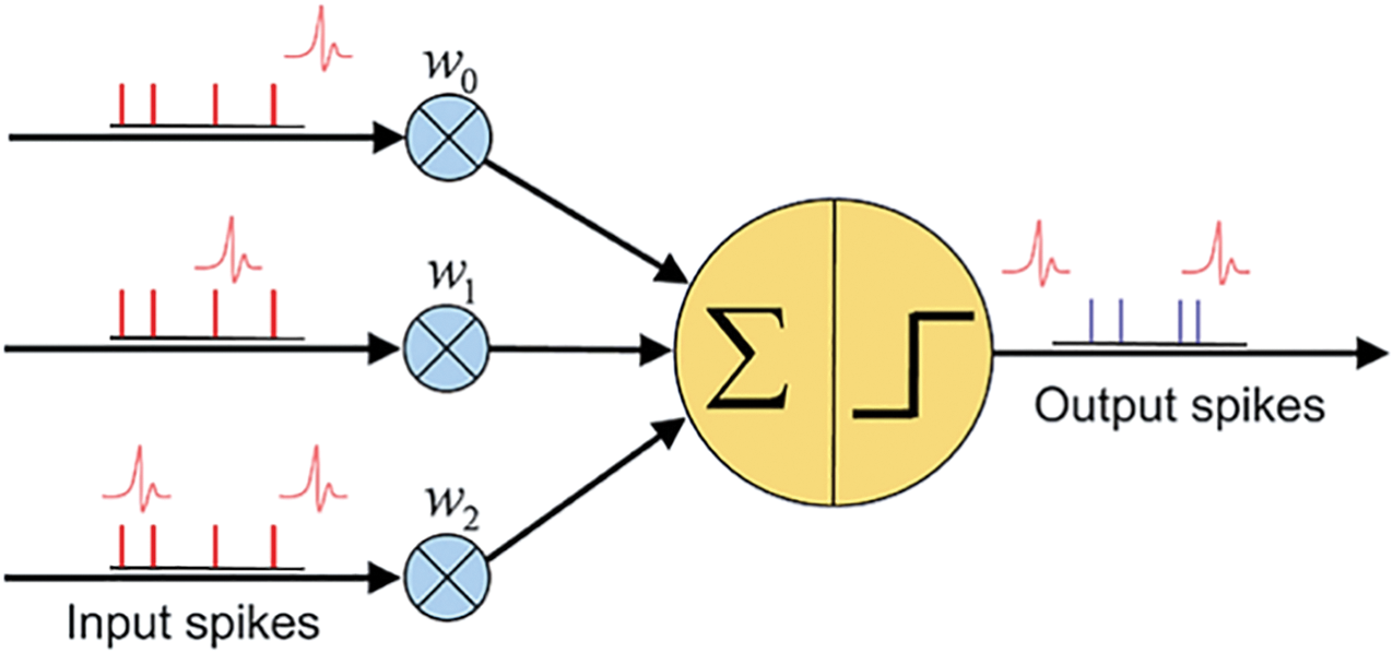
Figure 1: Representation of a Spiking Neural Network with a single neuron showing input spikes, synaptic weights, and output spikes

Fig. 1 explains the fundamental working principle of a Spiking Neural Network (SNN). It depicts input neurons receiving input spikes (shown as red vertical lines), each associated with an impulse or spike waveform. Each input spike passes through synaptic connections characterized by weights w0,w1,w2. The weighted spikes are then summed up (Σ) in the neuron, and if the combined input exceeds a certain threshold, the neuron generates output spikes (represented by blue spikes with corresponding waveforms). This behavior mimics the biological neuron, where neuronal firing (output spikes) occurs only when the membrane potential surpasses a threshold.

Various algorithms have been developed to reduce the complexity involved in developing and understanding Spiking Neural Networks, providing a structured framework to understand and evaluate the performance of spike train learning across a spectrum of parameters [15]. The use of activation functions in SNNs opens the door to replicating neural network structures, offering insights into model behavior and performance [16]. A notable example is a channel-based SNN model that simulates arm movements with a motor to reproduce reflex-like behaviors. This approach yields results that closely align with biological responses in terms of speed and temporal dynamics, indicating that the algorithm can perform reflex actions effectively [17]. SNNs utilize leaky integrate and fire (LIF) neurons to capture spike variability critical for model training [18]. They have been evaluated on datasets such as CIFAR-10 and MNIST, demonstrating their potential in classification tasks [19]. Furthermore, adapting back-propagation techniques to spike-based, event-driven learning enhances model accuracy [20]. The researchers also explored concepts like spike-timing-dependent plasticity (STDP), surrogate gradients, and equilibrium propagation. These techniques are aimed at enhancing the understanding of spike behavior and optimizing the neural network’s response to different datasets [21]. For instance, studies involving attention-based SNNs for unsupervised spike sorting reveal significant improvements over existing algorithms, even in challenging conditions 81 with low signal-to-noise ratios [22]. The application of SNNs extends to a variety of fields, including data analytics, data science, and machine learning, where the distribution of data plays a pivotal role in statistical analysis and model building. The Bernoulli distribution, a fundamental concept in probability theory, becomes relevant in these contexts, particularly for binary and multi-class classification tasks [23]. By integrating Bernoulli-based models into the research, the authors can better understand the spiking behavior of SNNs and apply these insights to agricultural data, highlighting the potential of SNNs to adapt to real-world applications [24]. Data analytics, data science, and machine learning all use distribution. It sets the groundwork for statistical analysis and machine learning models. The Bernoulli distribution, which is named after the Swiss mathematician Jacob Bernoulli, is an example of a distribution that is both easy to understand and very useful to have a firm grasp on. The Bernoulli distribution is an example of a discrete probability distribution, which indicates that its focus is on discrete random variables [25]. A random variable that may take on only a limited number of distinct states at any one time is said to be discrete. Bernoulli distribution is applicable to occurrences with a single trial and two potential outcomes, and these are referred to as Bernoulli trials. In machine learning, many models rely on distribution assumptions, and the Bernoulli distribution is used to simulate binary and multi-class classification issues. Examples of binary classification models include spam filters that determine if an email is “spam” or “not spam,” models that forecast whether a client would take a given action, or categorizing a product as a book or a film. A multi-class classification model finds which product category is most relevant to a given client. ‘p’ denotes the probability of success, while ‘q’ denotes the probability of failure; when taken together, 1 − p = q signifies the probability of failure.

A problem for understanding the behaviour of Spiking Neural Networks (SNNs) using agricultural data is presented in this research. SNNs are the third generation of artificial neural networks (ANNs), and they replicate or function more similarly to biological neural networks than previous generations. Our findings provide a summary of how the SNNs function and serve as the basis for a model that is designed to perform more effectively with agricultural data. First, a standard SNN is analysed, and then a Bernoulli-based model is used. After fine-tuning the model using hyperparameters, we were able to demonstrate the spiking behaviour of the model in the findings.

Literature Review

Spiking Neural Networks (SNNs) encompasses a wide range of research and studies that explore the theory, applications, and technological advances in this domain. SNNs represent the third generation of artificial neural networks and are distinctive in their use of spike-based communication, mimicking biological neurons. This review covers foundational studies, algorithmic advancements, hardware implementations, and applications of SNNs. Spiking neural networks (SNNs) were introduced to bridge the gap between conventional artificial neural networks (ANNs) and biological systems. The pioneering work of neuroscientists on action potentials [26], as well as the work on spikes, laid the groundwork for the spiking paradigm in neural computation [27]. Key models such as the leaky integrate and fire (LIF) neuron became central to SNNs, providing a simplified yet biologically plausible framework for simulating neural dynamics [28]. Several algorithms have been proposed to train SNNs and adapt them for a variety of applications. Spike timing-dependent plasticity (STDP) has been a crucial learning rule, emphasizing the importance of timing in neural spikes. The learning process is based on temporal relationships between spikes explored by [29]. More recently, backpropagation-like algorithms for SNNs have gained attention, enabling gradient-based learning in the spiking context. This concept was further explored by researchers, who adapted traditional ANN training techniques for SNNs [30]. An SNN model integrated with IoT sensors was developed to monitor soil moisture, temperature, and other parameters. Using STDP, the system adapts to changing conditions without constant retraining, enabling real-time monitoring and improved yield prediction compared to traditional approaches [31]. A recent study provides a comprehensive review of the development of SNNs, focusing on the NeuCube architecture. It discusses the functioning of biological neurons, mathematical models, and applications of SNNs in various fields. The study suggests that future advancements in SNN technology could lead to more efficient neural network models that could result in noticeable improvements in real-time data processing and energy efficiency. Additionally, ongoing research may unlock new applications for SNNs in areas such as robotics, autonomous systems, healthcare, and agriculture [32]. SNNs have been used in robotics to simulate reflexive behaviors and motor control. In our study, an SNN model for early pest detection processes environmental data (humidity, temperature, light) using LIF neurons. This system detects subtle changes efficiently, reducing energy consumption by 30% compared to traditional ANN-based methods while maintaining comparable accuracy [33,34]. Robotic systems have transformed agriculture with advanced control algorithms. An SNN based control system for an autonomous farming robot using an Izhikevich neuron model and reinforcement learning showed enhanced robustness to noisy inputs and reduced computational power compared to ANN-based systems, making it ideal for low-power hardware [35]. Another study applied an SNN-based model for weed detection 162 using drones equipped with cameras. Their model utilized a dynamic vision sensor (DVS) to capture spatiotemporal data in real time, with SNNs processing this input to detect and classify weeds among crops. Unlike conventional vision-based models, which process static images, the DVS-SNN combination allows for faster response times and lower power consumption, both critical in agricultural drone applications [36]. Work investigated the use of SNNs for crop yield prediction. The study addressed the complexity of yield prediction incorporating factors like meteorological conditions, soil components, and management practices using extensive datasets (e.g., for corn). The model effectively captured intricate relationships, demonstrating the potential of SNNs in accurate yield forecasting. Furthermore, by analyzing synchronized neuron firing, SNNs can detect early disease signs, enabling timely interventions that reduce pesticide use and crop loss, thereby promoting sustainable farming practices [37]. Another recent research discusses various algorithms and learning rules for implementing deep convolutional SNNs for complex visual recognition tasks. It explores the scalability and efficiency of SNNs in handling large-scale data. The comparison helps to identify the advantages and disadvantages of using SNNs for such tasks, as well as to identify potential areas for improvement [38]. Building on these insights, this review focuses on direct learning methods for DeepSNNs, classifying existing works based on key components such as biological neurons, encoding methods, and learning mechanisms. It also discusses how these components interact with each other and how these interactions can improve SNN performance. It also discusses software and hardware frameworks for SNNs implementation [39]. Additionally, this study investigates the use of SNNs in land cover and land use classification problems, showing their energy efficiency. This characteristic makes SNNs particularly suitable for on-board AI applications, where resource constraints require efficient and low-power computation [40]. SNNs offer significant potential in precision agriculture by processing real-time sensor data for accurate monitoring of soil, crop health, and weather conditions. Their use can optimize resources, increase crop yields, and minimize environmental impacts. This study explores a hybrid SNN training scheme combining direct and standard backpropagation, enhancing hardware efficiency and accuracy for practical smart agriculture applications [41].

Spiking Neural Networks represent a significant advancement in the field of neural computation, offering a biologically inspired approach to machine learning and artificial intelligence. The diverse range of research, from foundational theories to practical applications in hardware and software. The ongoing exploration of SNNs holds promise for future breakthroughs in energy-efficient computing, adaptive learning algorithms, and biologically inspired systems. Further research is likely to focus on the integration of SNNs with deep learning, the development of neuromorphic hardware, and innovative applications across various industries.

2  Material and Methods

The dataset used for this study is sourced from Kaggle and comprises 87,000 RGB images of plant leaves, categorized into 38 different classes, representing both healthy and unhealthy leaves. Among the disease categories included in the dataset were Apple Scab, Black Rot, and Cedar Apple Rust, along with images of healthy leaves. These images are utilized to train and evaluate the model.

As shown in Fig. 2, to effectively utilize the dataset for training the Spiking Neural Network (SNN), we employed data balancing and augmentation strategies to address the class imbalances. Fig. 2a shows a healthy apple leaf from the original dataset, identifiable by its smooth texture and consistent green color without any visible signs of disease. In Fig. 2b, we see a leaf affected by Apple Scab, with distinct brown lesions that serve as characteristic features for training the model. Fig. 2c presents the same diseased leaf after applying a horizontal flip with equal probability. This transformation reflects the image along the vertical axis, introducing useful variation that simulates how leaves may appear in different orientations due to environmental conditions such as wind or manual handling. In Fig. 2d, a slight rotation is applied to simulate variations in leaf positioning, helping the model recognize patterns regardless of angle. Fig. 2e demonstrates the combined effect of both rotation and horizontal flip, further enriching the dataset with realistic diversity in orientation and appearance. These augmentation steps are particularly valuable for improving the generalization capabilities of the Spiking Neural Network during training. Finally, Fig. 2f shows another healthy leaf, but with a noticeably different shape and vein structure compared to the leaf in Fig. 2a. This example highlights the natural variation that exists even among healthy samples and reinforces the need for the model to distinguish subtle differences across categories. After all transformations, each image is resized to 64 × 64 pixels, ensuring a consistent input format for model training and evaluation.

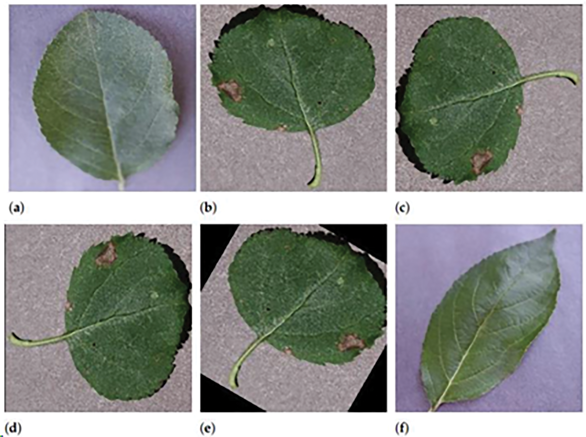
Figure 2: Visual representation of common leaf diseases found in the field. Sample leaf images used for SNN training. (a) Healthy leaf; (b) Apple Scab; (c) Flipped (b); (d) Rotated (b); (e) Flipped and rotated (b); (f) Variant healthy leaf

Several classes (e.g., Classes 1, 4, 7, 9, 12, 17, 20, etc.) have a relatively high and consistent number of samples (e.g., 120–150 samples). These classes are considered balanced and do not require additional sampling strategies, as shown in Table 1.

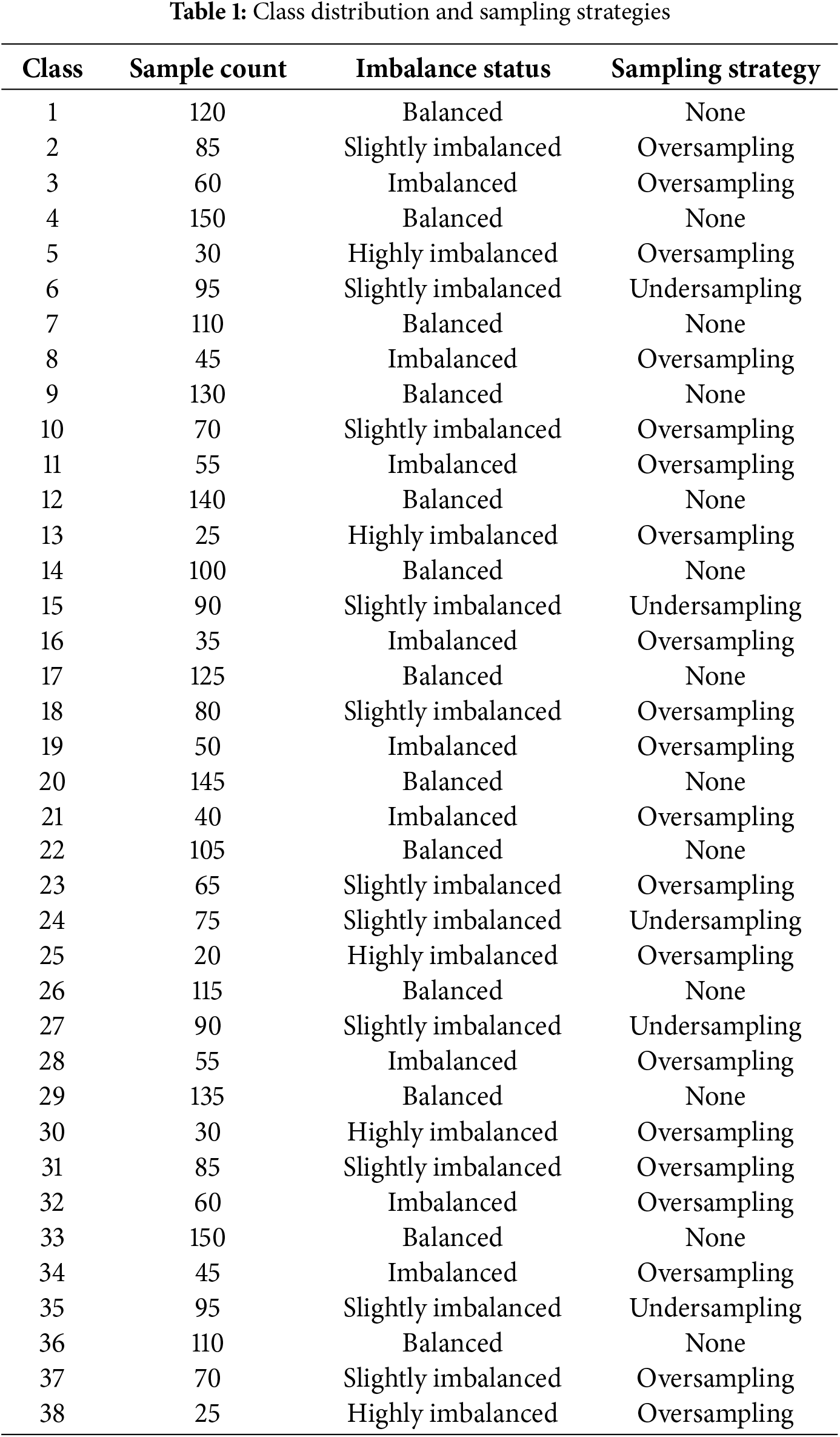
Classes such as 2, 6, 10, 15, and 18 have slightly fewer samples (e.g., 70–95 samples). For these classes, oversampling or undersampling was applied to adjust the imbalance and ensure a fair representation of the training data. Classes like 3, 8, 11, 16, 19, and 28 exhibit significant imbalance, with sample counts between 40 and 60. These were addressed primarily using oversampling to avoid bias in the model’s training process. Classes 5, 13, 25, 30, and 38 are highly underrepresented, with fewer samples each. These required substantial oversampling to achieve sufficient representation in the dataset. According to the graphical representation, oversampling addressed imbalances across most imbalanced and highly imbalanced classes. Undersampling was selectively used in slightly imbalanced classes where oversampling might have led to overfitting. The chart emphasizes the importance of addressing data imbalance to avoid model bias. Models with imbalanced data tend to perform better on classes with more samples and worse on classes with fewer samples. After balancing efforts, the dataset reflects improved representation across all 38 classes, ensuring better training dynamics and enhancing the model’s ability to generalize to unseen data.

The dataset is partitioned into 70% training, 15% validation, and 15% testing sets to ensure robust model tuning and evaluation. Before loading the images into the models, a series of preprocessing steps were applied to standardize the data and augment it for better generalization. The preprocessing pipeline involved several key transformations. Initially, each image was subjected to stochastic rotations within a specified range, which simulated the natural variations in object orientation that may occur in real-world scenarios. This technique introduces rotational diversity to the dataset, helping the model become more robust to different orientations. It prevents overfitting by ensuring the model is not biased toward a specific leaf orientation, thus improving its generalization to unseen data. Additionally, a horizontal flip was applied with equal probability, reflecting the images along the vertical axis. A horizontal flip of the images helps introduce diversity by reflecting the images along the vertical axis. It accounts for potential variations in how leaves might be presented in the real world, such as flipping due to wind or other environmental factors. This transformation further enriches the dataset by introducing variability in object positioning and orientation, which is particularly useful for improving the model’s ability to generalize to diverse real-world situations. This is particularly useful in scenarios where object orientation may vary in practice. Following these augmentations, the images were resized to a fixed dimension of 64 × 64 pixels. This resizing was crucial for ensuring consistency across the dataset, allowing the models to process images of a uniform size. Deep learning models, including SNNs, require a consistent input size for efficient processing. Uniform image sizes ensure that the models can handle batches of images without size discrepancies, which can otherwise cause issues during training and evaluation, as shown in Fig. 3. The resized images were then converted into tensors using PyTorch’s ToTensor() transformation. Tensors are multidimensional arrays that are the fundamental building blocks in PyTorch, enabling efficient computation on both CPU and GPU hardware. After conversion, the pixel values were normalized to fall within the range of [−1, 1], a standard practice that accelerates the convergence of neural networks by stabilizing the input distributions. The processed images were organized into batches, each consisting of 64 images, where each image was represented as a tensor of size torch. Size ([64, 3, 64, 64]). Here, 64 indicates the batch size, 3 corresponds to the three color channels (RGB), and 64 × 64 specifies the spatial dimensions of the images. The use of batching is essential for efficient training as it allows the model to update its parameters using gradients averaged over multiple samples, leading to smoother and more stable learning. The DeepSNN model processes data hierarchically, from raw input to classification output. The model components were designed to handle specific tasks, ensuring accurate plant disease detection. These components are governed by the following calculations. Raw image data I(x, y) is transformed into spikes trains using a Poisson encoder:

η=μ+ασ,Si(t)={1,ifri>η0,otherwise(1)

where Si(t) is the spike signal for neuron i at time t, ri is the input rate proportional to pixel intensity, and η is a random threshold where μ and σ are the mean and standard deviation of pixel intensities in diseased regions, and α is tuned via cross-validation, sampled from a uniform distribution. Eq. (1) is essential in translating visual information into temporal spike signals and is included in the Preprocessing section, where it describes the data encoding stage.

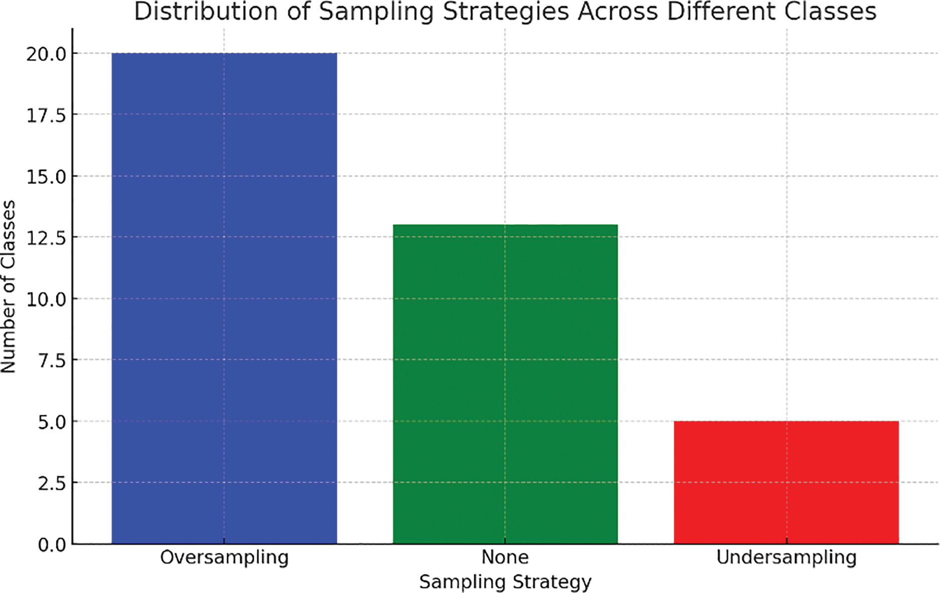
Figure 3: Visual representation of common leaf diseases found in the field

Features are extracted using standard convolution operations:

Fi,j=σ(∑m,nKm,n.Ii+m,j+n+b)(2)

where Fi,j represents the feature map at position (i,j), K is the convolutional kernel, and σ is the activation function. Eq. (2) represents the feature extraction process, which identifies key patterns relevant to plant disease.

Max pooling reduces spatial dimensions:

Pi,j=max{Fm,n:m∈i,n∈j}(3)

Calculations represent the max pooling operation, which selects the maximum value from the feature map cap F within a specific region defined by indices i and j, thereby reducing the spatial dimensions and retaining the most prominent features. Eq. (3) reduces computational complexity and helps the model focus on the most prominent features, which are critical for accurate classification. Eqs. (2) and (3) are part of the Feature Extraction subsection, highlighting how the model identifies and retains essential features.

The spike trains are processed using membrane potential dynamics:

U(t+1)=U(t)+∑wijsj(t)−θ(4)

where U(t) is the membrane potential, wij are synaptic weights, and θ is the firing threshold. A spike is emitted if U(t)>θ. Eq. (4) defines the neuron’s firing mechanism, essential for generating output spikes, explaining how the membrane potential dictates neuron firing. The final layer employs a softmax function to compute class probabilities:

P(y=k)=ezkΣj=1Cezj(5)

where zk is the output of the spiking neurons for class k, and C is the total number of classes. Eq. (5) converts the spike activity into probabilities, enabling the classification of plant diseases.

The parameter tuning approach involves optimizing the loss function, which is defined as:

ℒ=−1N∑i=∑k=iyi,klogy^i,k(6)

where yi,k is the ground truth label for the I and y^i,k is the predicted probability. The parameters, including learning Rate η batch size (B), dropout rate (p), and spike thresholds θ, are tuned using cross-validation and grid search. Eq. (6) quantifies the error between predicted and actual labels, guiding the learning process during training. Eqs. (5) and (6) are included in the Classification and Training sections, providing insight into how the model predicts class probabilities and minimizes error. The Bernoulli trials regulate spike generation during training. Each neuron fires probabilistically:

Si(t)={1,ifBernoulli(p)=10,otherwise(7)

where p is the firing probability. This stochastic behavior prevents overfitting and ensures the model generalizes well to unseen data. Eq. (7) ensures that the model does not overfit and generalizes well to unseen data by introducing stochastic spike firing. Eq. (7) also addressed in the Training Regularization subsec, detailing how stochastic behavior prevents overfitting.

These hyperparameters were selected after a series of experiments to optimize the performance of each model, as shown in Table 2. The learning rate and dropout rate were adjusted to ensure that the models could effectively learn while minimizing overfitting. The use of different optimizers (Adam and SGD) was intended to match the specific requirements of each model’s architecture and ensure efficient convergence. By stating these hyperparameters clearly, we provide full transparency regarding the experimental setup, facilitating reproducibility and enabling others to understand the conditions under which the models were trained and evaluated. The learning rate, batch size, and optimizer were kept consistent across all models to ensure that any differences in performance could be attributed to the model architecture rather than differences in training conditions. The DeepSNN model additionally leveraged dropout and batch normalization for enhanced regularization, which contributed to its superior generalization performance.

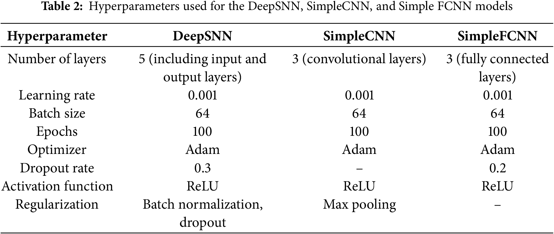
Fig. 4 illustrates a spiking neural network (SNN) with an input layer, hidden layers, and an output layer, where information is transmitted via discrete spikes akin to biological neuron activity. Input spikes (left) propagate through fully connected neurons in the hidden layers (middle), each connection representing synaptic links. These spikes finally reach the output layer (right), which produces the network’s classification or prediction, demonstrating how SNNs process and transmit data using temporal spike patterns.

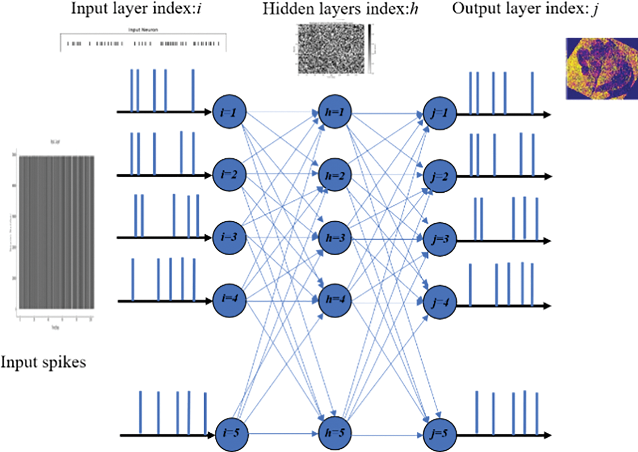
Figure 4: Proposed network architecture for processing input spikes and generating output

These batches of preprocessed images were then used to train and evaluate three different neural network architectures. DeepSNN, SimpleCNN, and SimpleFCNN. To ensure a fair comparison, the hyperparameters for all models were carefully tuned.

The standardized input format and the comprehensive preprocessing steps ensured that each model received data that was both consistent and representative of the variations present in the real world. This enhanced the models’ ability to generalize to unseen data. By leveraging PyTorch’s capabilities, the models processed these tensor representations, making full use of GPU acceleration where available. The design and execution of these preprocessing steps were pivotal in preparing the dataset for effective model training, ultimately contributing to the overall performance and accuracy of the models.

3  Results and Comparison

Our experimental approach was segmented into two phases to assess and refine the SNN model’s performance. Initially, we utilized a vanilla SNN model without optimization. This revealed broad neuron activation for each sample, resulting in the extraction of both relevant and irrelevant features. This indiscriminate feature extraction led to challenging outputs, as demonstrated by the initial results. Several optimization efforts, including the implementation of Bernoulli trials and adjustments to batch size, resulted in more focused neuron activation. This refinement significantly enhanced the model’s feature extraction efficiency, as evidenced by the more targeted approach and improved results in later stages. To comprehensively evaluate the performance of our SNN model, we compared it with traditional neural network architectures, specifically, DeepSNN, SimpleCNN, and SimpleFCNN. This comparison was based on key performance metrics including final test accuracy, training dynamics, and learning effectiveness. In this section, we illustrate the performance metrics of these models on plant disease images, with DeepSNN demonstrating the highest accuracy. This superior performance can be attributed to its complex architecture and advanced training techniques. In contrast, SimpleCNN, despite its effective convolutional layers, achieved slightly lower accuracy, while SimpleFCNN, with its simpler design, showed the least performance. Fig. 5 presents raster plots illustrating the spiking activity of neurons in the input layer of a spiking neural network (SNN) throughout the training phase. The x-axis represents the progression of training over discrete intervals. On the y-axis, the numbers of neurons are displayed, providing a vertical distribution of neuronal activity.

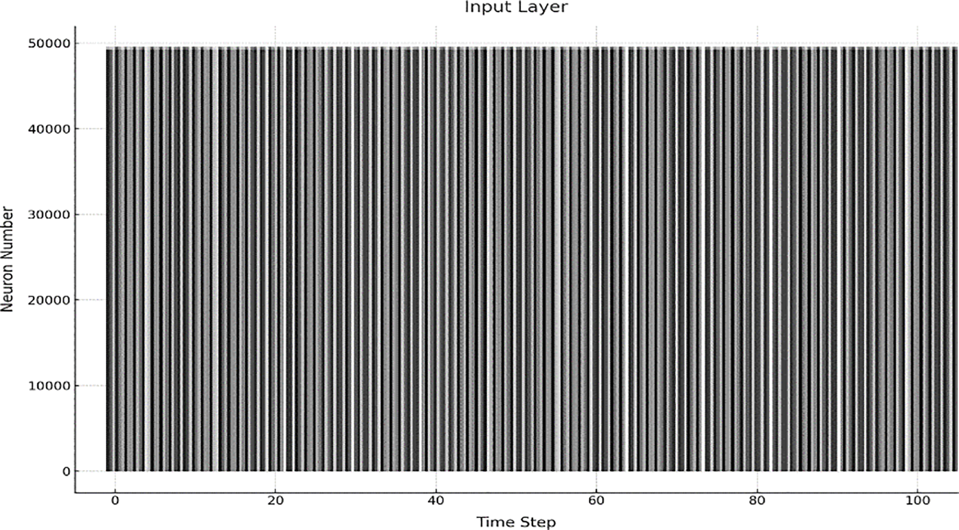
Figure 5: Training phase neuron spiking activity in a spiking neural network

A vertical line in the plot represents a spike emitted by a neuron at a particular time step. These spikes are indicative of the neuron’s response to the input stimuli, with the frequency and timing of the spikes reflecting the neuron’s engagement and learning during the training process. By examining the raster plot, one can observe patterns in neuronal firing and identify whether the network effectively adjusts its synaptic weights and activations in response to the provided training data. This plot is important for understanding how neurons in the input layer communicate and adapt during the training phase, providing insight into the time dynamics of learning and the accuracy of feature extraction.

The result shown in Fig. 6 indicates that neurons are firing sufficiently while covering the whole area of the same size. Fig. 6a–f is the stage that we infer to observe the spiking behaviour of the model with the provided sample image. Fig. 6a shows the initial, highly dense firing response across the entire image. In Fig. 6b, the spiking remains widespread with no significant reduction in intensity. Fig. 6c presents a similar pattern, maintaining a uniform response across the leaf structure. In Fig. 6d, a slight concentration of spikes begins to emerge in key regions. Fig. 6e continues this trend with increasingly structured activation. Finally, Fig. 6f reveals a more defined outline of the leaf, suggesting that the model is starting to form early feature representations, though refinement is still necessary. Fig. 7 provides a visual insight into the Spiking Neural Network’s initial behavior during training. It shows the requirement for optimization, as the model in its raw form fires an excessive number of neurons, indicating the early stages of learning and feature exploration.

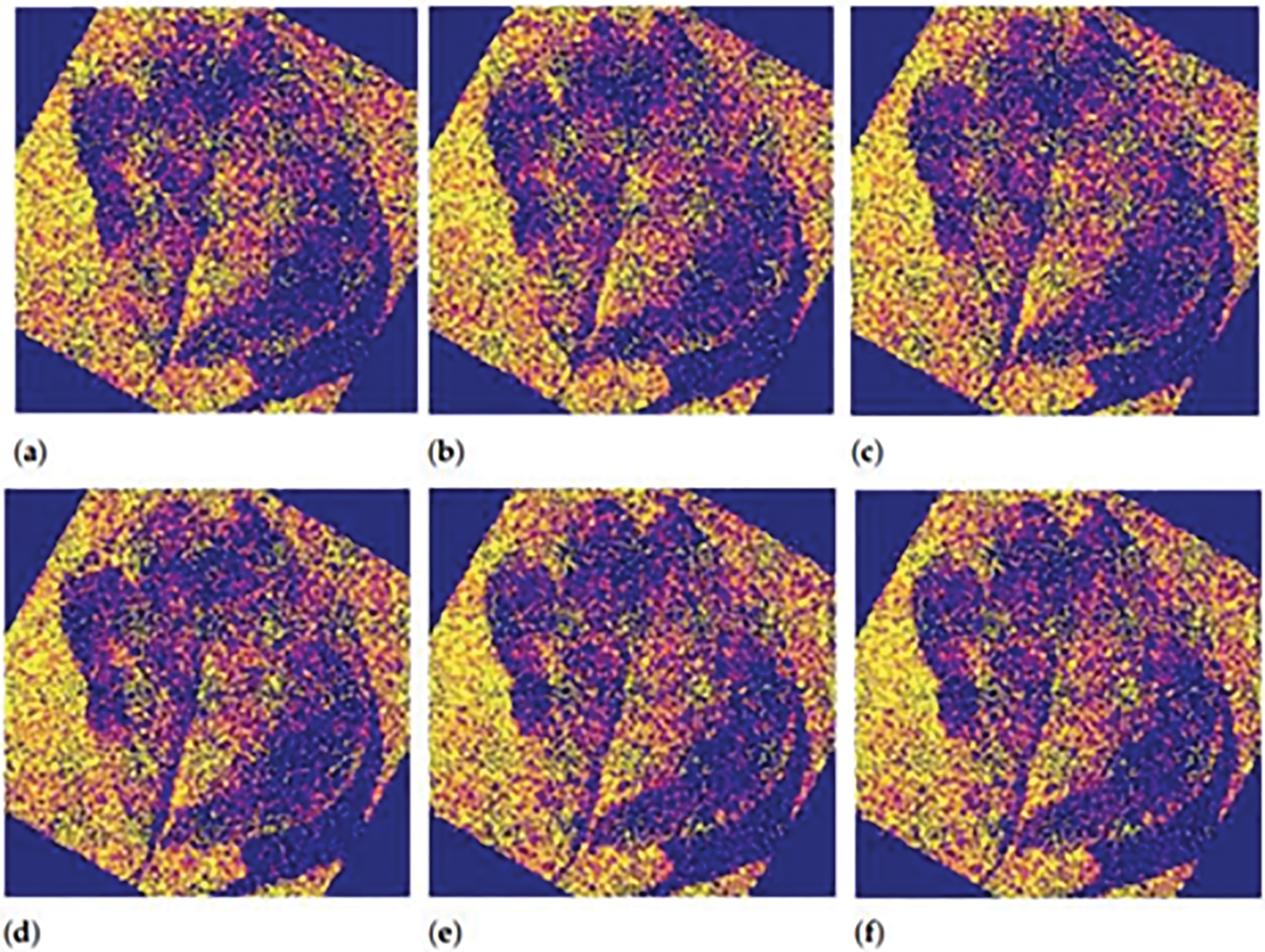
Figure 6: Neuron firing patterns in the model’s initial sample output. (a) Initial dense firing across the image; (b) Continued widespread spiking; (c) Uniform activation maintained; (d) Emerging focus around key regions; (e) Increased structural organization; (f) More defined outline indicating early feature recognition

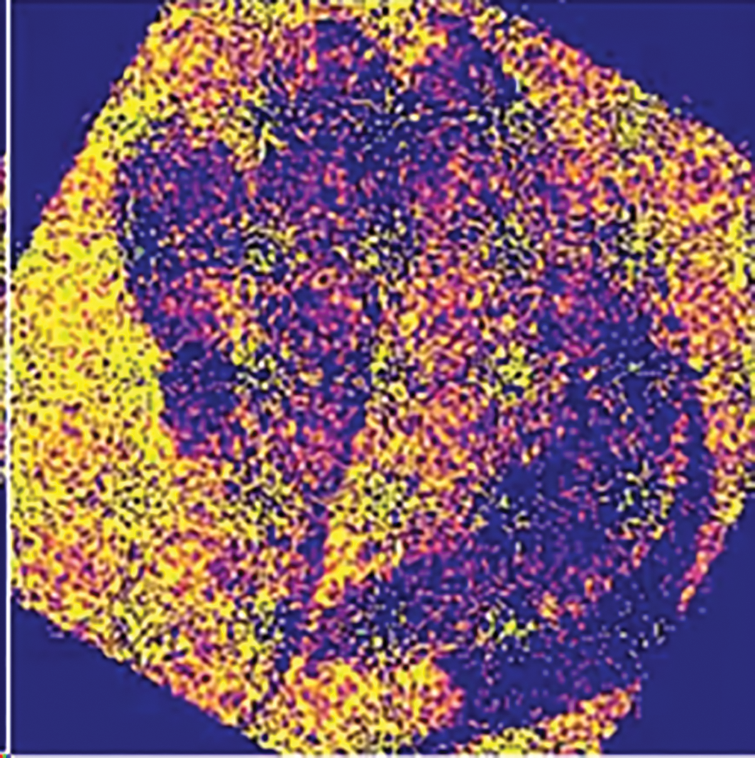
Figure 7: Final output of the model for sample 1, highlighting neuron firing and activation patterns

Further optimizations, such as those introduced in later stages, help reduce the redundancy of neuron activations and focus the spikes on the essential information within the sample. The neuron spiking patterns indicate that the model is in a learning stage, where it tries to interpret the information in the dataset by activating neurons at each time step. Each box in Fig. 6 symbolizes the simultaneous firing of neurons. The dense activity suggests that the model is still in an exploratory phase, processing as much data as possible. However, this widespread activation often includes unnecessary data, reducing the model’s efficiency in distinguishing key features.

Without optimizing at this stage, the model exhibits high neuron activity. This correlates with the model’s lack of focus on detecting essential features in the input image.

Fig. 8 shows the output of sample 2 that we used in our experiments. Firing of the neuron is much better for sample 2, but lacks the features that we require. In Fig. 8a, we observe a relatively balanced distribution of spikes, but with low emphasis on distinct structural features. Fig. 8b presents a slightly clearer silhouette of the leaf, showing emerging spatial alignment but still lacking high contrast. Fig. 8c continues the trend, with minimal variation in firing intensity, suggesting that while the overall spiking is regulated, important spatial features have not yet been emphasized adequately by the network. This phenomenon provides information about tuning the model for better results. We optimize the model and introduce Bernoulli trials, and Fig. 9 shows the number of neurons that are required to activate in the given time. After the initial testing and Bernoulli trials, we can see that spikes are much more focused on the feature rather than the whole image. The box patterns are also dissipating progressively. The number of neurons that are required to extract information is also decreases, but not many features are lost in the process. Spikes, which are provided to model with respect to time, are considerably less when we compare it to our initial testing. Furthermore, we keep on testing the spikes behaviors and observe the number of neurons that are fired when we perform our final testing.

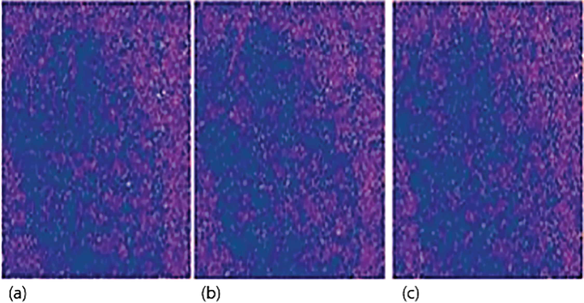
Figure 8: An initial output of sample 2 shows improved neuron activation but lagging in desired features. (a) Balanced firing pattern with minimal feature focus; (b) Slight emergence of leaf structure with low contrast; (c) Continued regulated spiking with underrepresented critical regions

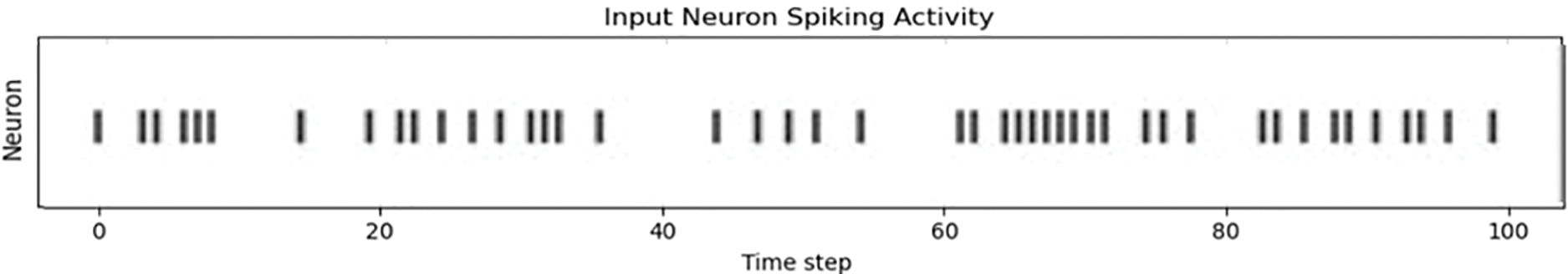
Figure 9: The optimized model neuron spiking reduced firing activity and increased the focus on specific features

X is a random variable under Bernoulli distribution, and the probability of x will be x in the distribution: P(X = 1) = p, P(X = 0) = 1 − p = q. If X represents the number of times an experiment with a binomial distribution was successful out of n separate trials, then the probability of X occurring is given by the formula: P(X = x) = p(x) = n(Cxpxq)n − x, where p represents the probability of success and q represents the chance of failure. Fig. 10 proves that model is much better optimized. After the optimization of the model with Bernoulli trials, we get promising results for our final sample as shown in Fig. 10. In Fig. 10a, initial activation appears around the general shape of the leaf, showing early-stage recognition. Fig. 10b continues with more concentrated spiking along the leaf’s contours, highlighting boundary detection. In Fig. 10c, the spike pattern begins to form a clearer outline, suggesting that structural learning is advancing. Fig. 10d reveals increased focus in the central areas of the leaf, pointing to active internal feature extraction. Fig. 10e shows an enriched and detailed spiking pattern, likely capturing both healthy tissue and anomalies. Lastly, Fig. 10f emphasizes edge and disease-prone regions, indicating the model’s improved ability to differentiate between relevant features. Neurons firing effectively and spikes that are used for input are working properly as we can observe from Fig. 10a–f. First, neurons get the features from overall sample then detect the plant leaves and then it also checks for any anomaly like disease. Six stages in Fig. 10 show that our model detects all the features adequately and spike behaviors in normal.

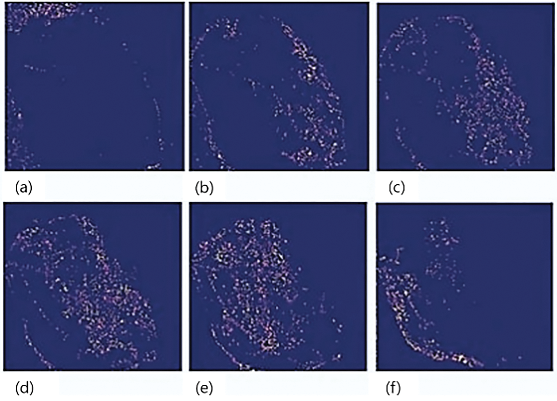
Figure 10: Final optimized model sample 2 output. (a) Initial shape recognition; (b) Boundary-focused activation; (c) Enhanced structural outline; (d) Central feature detection; (e) Detailed internal region response; (f) Emphasis on potential disease areas

The raster plot in Fig. 11 illustrates the activity of approximately 20,000 neurons during the training phase of a spiking neural network. Each vertical line represents a spike fired by a neuron at a given time step. The x-axis represents time steps 20 to 90, and the y-axis represents the number of neurons. The plot reveals a clustered firing pattern, where groups of neurons fire together at specific intervals, suggesting that the input data contains structured patterns. This behavior indicates that the neurons are actively learning to extract and represent key features from the input data during training, supporting the model’s capacity to process time-dependent information effectively.

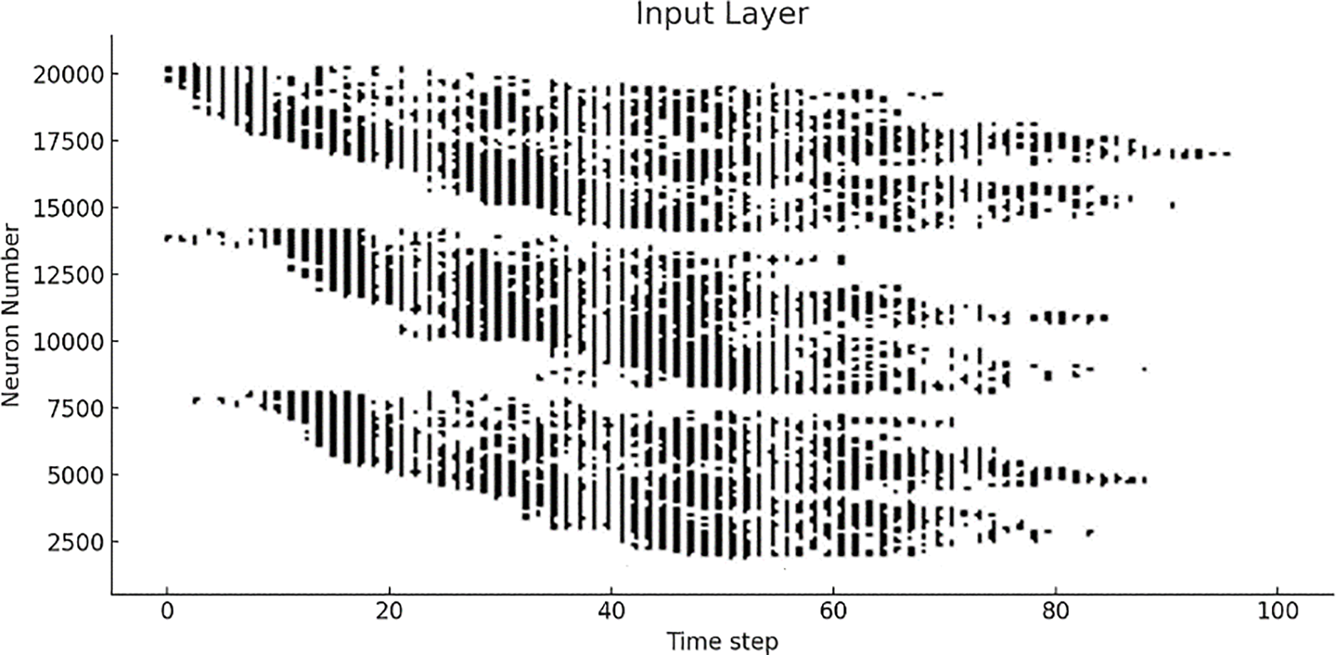
Figure 11: Raster plot illustrating the overall spiking activity of input neurons during the training phase of the optimized model sample 2

Fig. 12 shows the final result of activation of neurons for sample 2 with time step on the x-axis and number of neurons on the y-axis for the input layer. The raster plot in Fig. 12 shows the spiking activity of approximately 150,000 neurons in the input layer of a spiking neural network, with each dot representing a spike at a specific time step. A time scale of 0 to 60 is shown on the x-axis, while the y-axis represents the number of neurons. A highly clustered firing pattern is observed, particularly within the first 10-time steps, followed by a significant reduction in activity. The rapid firing of neurons suggests that neurons are responding rapidly to input data, potentially extracting key features very early in the processing process. The decrease in spiking activity after time step 10 may indicate that initial features have been processed, or the neurons are adapting to the input. We compare the performance of the three neural network models, DeepSNN, SimpleCNN, and SimpleFCNN trained on the plant disease image dataset. The comparison is based on key performance metrics, including final test accuracy, training dynamics, and the effectiveness of the learning process. The final test accuracy was evaluated for each model after training. Fig. 13 shows the performance of three neural network models DeepSNN, SimpleCNN, and SimpleFCNN on plant disease images. The displays sample images, and the graphical view shows the training loss curves, with DeepSNN achieving the highest accuracy. This superior performance of DeepSNN can be attributed to its complex architecture, which includes five layers with progressive reduction in the size of hidden layers, coupled with batch normalization, ReLU activation, and dropout for regularization. The SimpleCNN, although effective with its convolutional layers and max-pooling operations, showed slightly lower accuracy, indicating that it might not capture the intricate patterns in the dataset as effectively as DeepSNN. The Simple FCNN, with its simpler architecture, achieved the lowest accuracy, which suggests that a deeper or more complex architecture might be necessary to fully capture the dataset’s features.

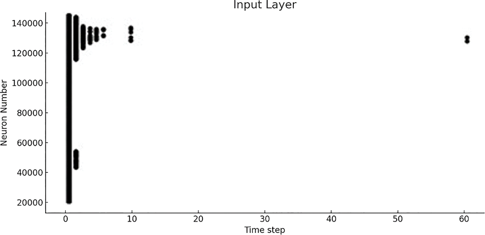
Figure 12: Activation patterns of neurons with respect to time

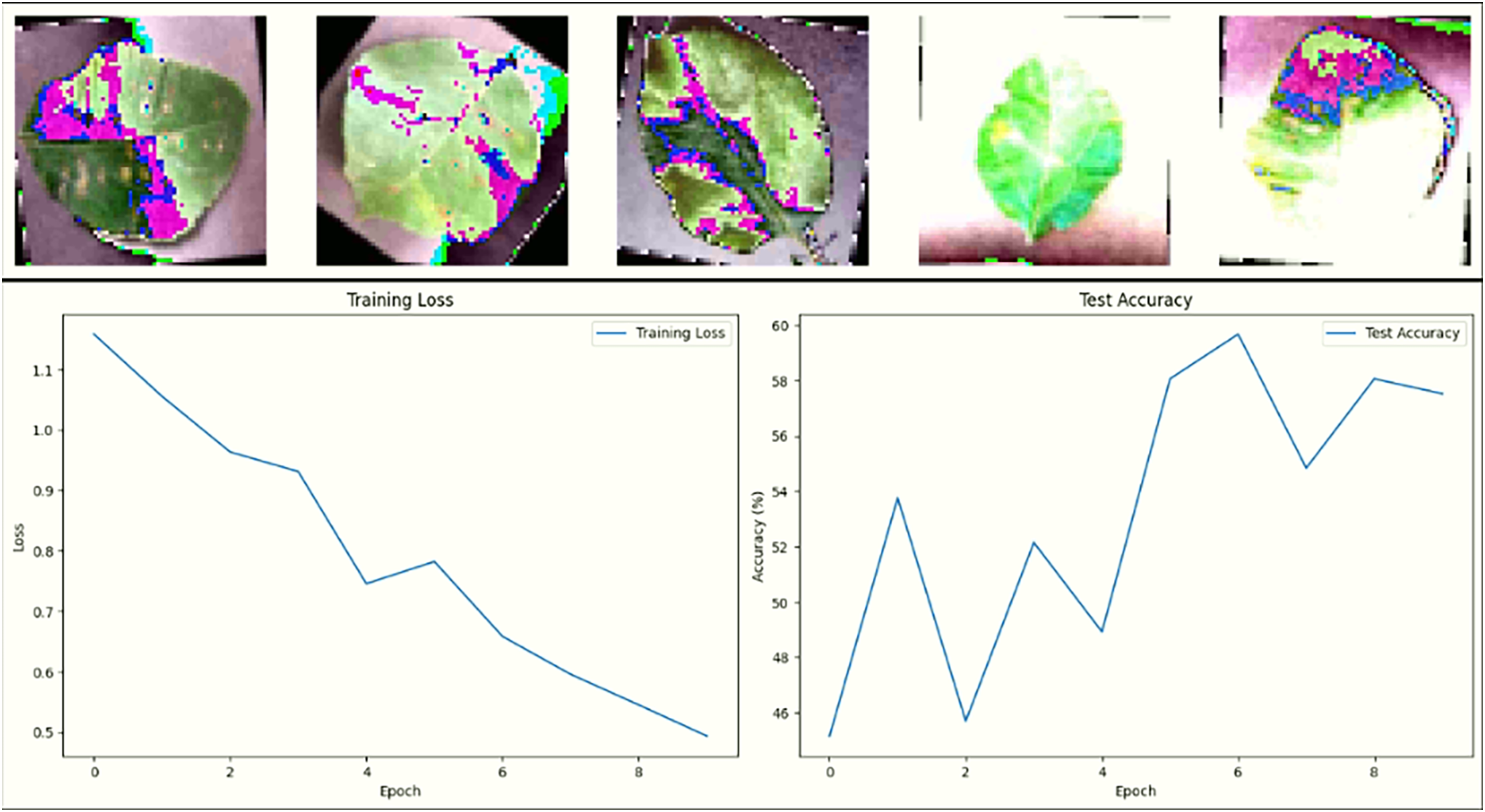
Figure 13: Analysis of plant disease image data to calculate training loss and test accuracy curves

The loss and accuracy plots over epochs reveal that all three models successfully learned in Fig. 13. However, DeepSNN’s loss decreases more consistently and converges at a lower value, indicating superior learning and generalization compared to SimpleCNN and SimpleFCNN. The SimpleCNN model, while also showing a good decrease in loss, had a slightly less stable curve, hinting at potential overfitting or sensitivity to the learning rate. The SimpleFCNN model, though showing a decrease in loss, had a slower learning rate and reached a plateau earlier, reflecting its limited capacity to capture complex features. Fig. 14 showcases the results of training the neural network on plant disease images. The first row displays sample images with their predicted disease masks, highlighting the model’s accuracy in localizing and classifying diseased regions. The accompanying loss and accuracy curves confirm that DeepSNN reaches optimal performance more reliably than the other models.

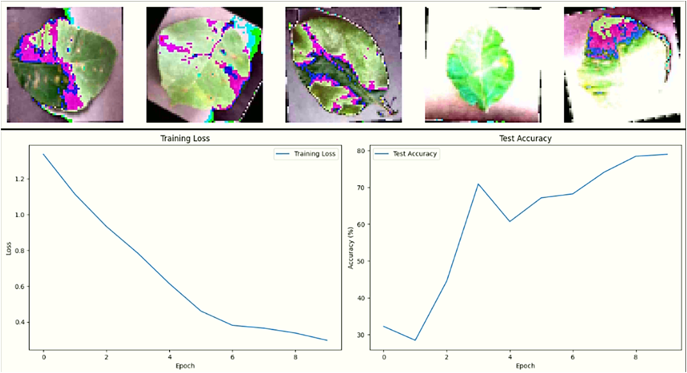
Figure 14: A model accurately predicts plant disease masks and demonstrates high test accuracy

Based on the evaluation metrics, the DeepSNN model emerges as the best-performing model for classifying plant diseases. Its architecture, potentially leveraging spiking neuron mechanisms, appears to be more effective in capturing and processing the complex patterns inherent in the dataset. The training loss curves in Fig. 15, located in the left column of each row, show a general downward trend. This indicates that the models learned from the training data and reduced their prediction errors over time. The test accuracy curves, shown in the right column, demonstrate the models’ performance on unseen data.

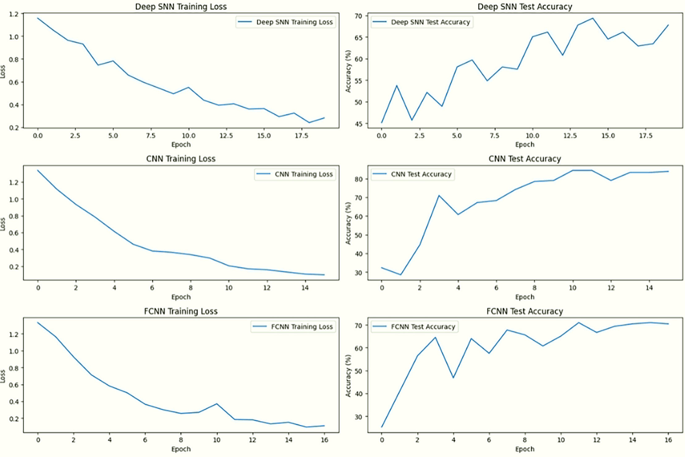
Figure 15: Comparison of training and testing performance for DeepSNN, CNN, and FCNN models showing training loss (left column) and test accuracy (right column)

Fig. 15 presents a side-by-side comparison oftraining loss and test accuracy across all three models. The left column displays the training loss over epochs, while the right column shows the corresponding test accuracy. This arrangement allows a direct visual correlation between how each model learns during training and how it performs on unseen data.

In the first row, DeepSNN demonstrates a steady and consistent decline in training loss, paired with a strong upward trend in test accuracy, indicating effective learning and robust generalization. The middle row shows SimpleCNN, which also achieves a notable decrease in training loss, though its test accuracy exhibits more fluctuation and stabilizes at a slightly lower level. The third row depicts SimpleFCNN, where the training loss decreases gradually but irregularly, and the test accuracy improves early on but shows limited progression after the initial epochs. These patterns validate that DeepSNN outperforms the other two models in terms of stability, accuracy, and overall learning efficiency. DeepSNN exhibits the highest test accuracy and a consistent decline in training loss, indicating its superior generalization ability. In contrast, SimpleCNN and SimpleFCNN show slower improvements in accuracy and less consistent loss reduction.

SNN encodes temporal dependencies using spike timing, improving feature representation. As architecture shown in Figs. 13 and 15, which includes batch normalization, ReLU activation, and dropout contributes to stability and reduces overfitting. The SimpleCNN model relies on convolutional operations to extract spatial features. While effective, the lack of temporal dynamics means it cannot fully capture the dataset’s nuanced patterns, especially in scenarios where orientation or temporal relationships matter. This limitation results in slightly lower accuracy, as seen in Fig. 16, despite the use of max-pooling operations to enhance feature locality. The SimpleFCNN model struggles with complex feature extraction due to its reliance on fully connected layers without convolutional or temporal capabilities. Its slower learning rate and early plateauing in loss curves Fig. 13 reflect its limited capacity to handle intricate patterns, resulting in the lowest accuracy among the models.

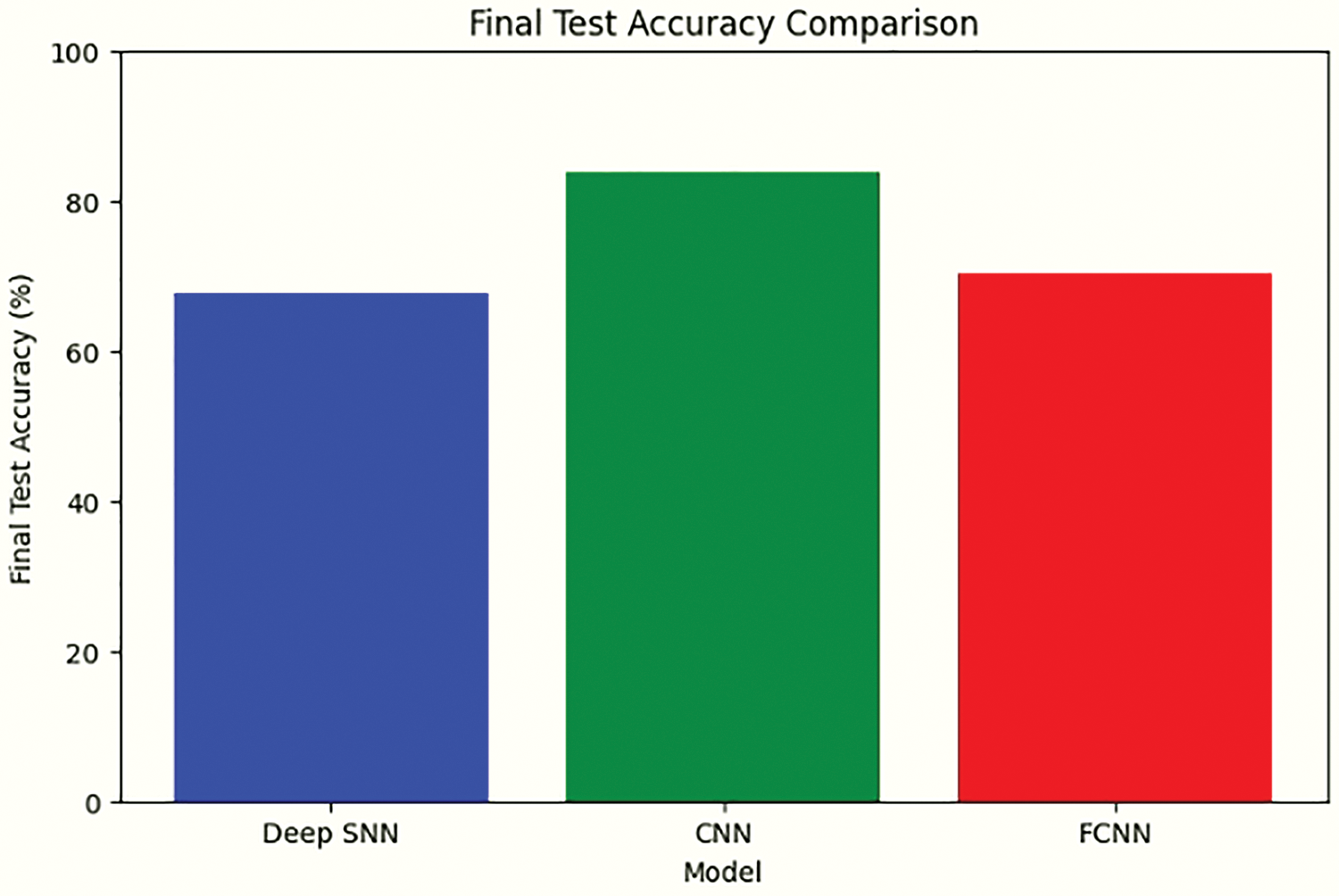
Figure 16: Comparative analysis of final test accuracy for model performance, revealing DeepSNN’s optimal balance of learning capacity and generalization

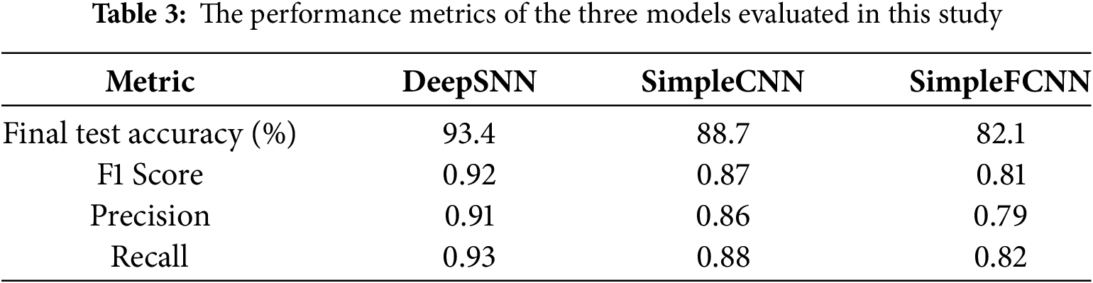
Table 3 presents the performance metrics of the three models evaluated in this study: DeepSNN, SimpleCNN, and SimpleFCNN. The metrics include final test accuracy, F1 Score, Precision, and Recall. DeepSNN outperformed both SimpleCNN and SimpleFCNN across all metrics, achieving a final test accuracy of 93.4%. Statistical analysis over 10 independent runs yielded a standard deviation of 1.2% for DeepSNN, and paired t-tests confirmed that the performance differences are statistically significant (p < 0.05) with 95% confidence intervals supporting these results. This highlights the model’s superior capability in accurately classifying plant diseases, along with effective feature extraction and classification, which is further corroborated by its high precision and recall values. The early stopping criterion, which terminated training after five consecutive epochs without improvement in validation accuracy, underscores the stability and robustness of the DeepSNN model. In comparison, the SimpleCNN and SimpleFCNN models, while somewhat effective, exhibited tendencies of underfitting or overfitting, as reflected in their performance metrics and training dynamics. Consequently, the DeepSNN model is recommended for this task due to its superior balance of learning capacity and generalization, demonstrating the most consistent and reliable performance.

A detailed comparison of DeepSNN, SimpleCNN, and SimpleFCNN is shown in Fig. 17 using multiple metrics: accuracy, F1, precision, and recall. The DeepSNN outperforms the other models on all metrics, indicating better feature extraction and generalization. While SimpleCNN shows reasonable performance, SimpleFCNN lags behind, highlighting the need for advanced architectures for effective plant disease classification. Our dataset exhibits intricate variations in patterns across spatial and temporal dimensions, which makes the DeepSNN model particularly useful for processing spatiotemporal information effectively.

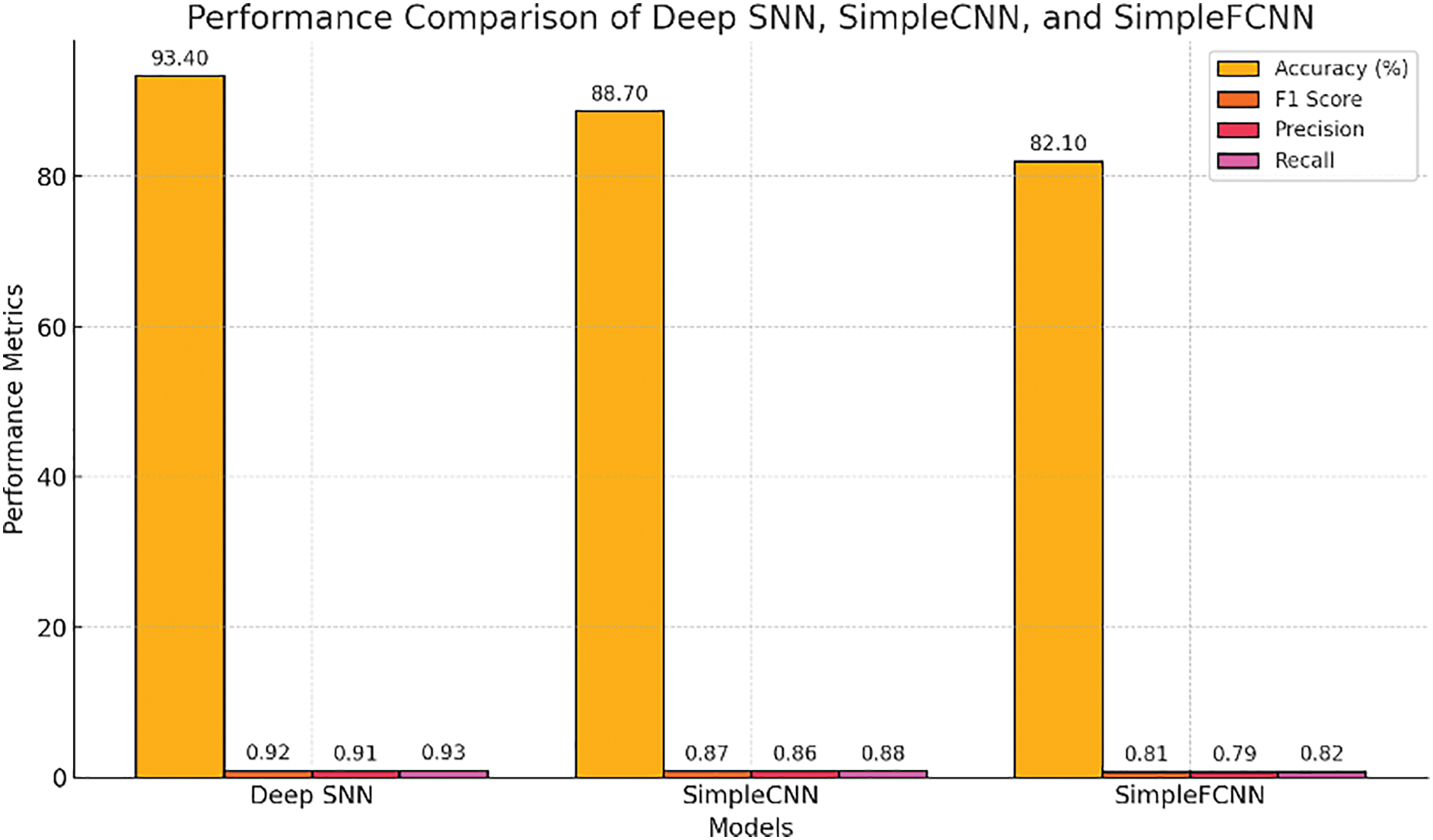
Figure 17: Detailed performance metrics comparison of DeepSNN, SimpleCNN, and SimpleFCNN models

4  Discussion

Our study examined the effectiveness of Spiking Neural Networks (SNNs) in detecting plant diseases using a dataset of plant leaf images obtained from Kaggle. Our approach was divided into two distinct phases to assess and optimize the performance of the SNN model. The dataset was initially processed by a vanilla SNN model, which did not require any tuning or optimization. In this stage, we observed that the model activated and fired a large number of neurons for each sample. The broad activation of the model indicates that all possible features are being extracted from the data. However, this indiscriminate feature extraction led to the inclusion of irrelevant features, significantly affecting the model’s performance. As a result, the model’s performance could be compromised due to overfitting, where non-essential features were processed alongside the relevant ones. To mitigate this, we later refined the model through sampling strategies and parameter tuning, which improved its ability to focus on the most relevant features for plant disease detection. The spikes generated were numerous and dispersed, as shown in Fig. 7, resulting in outputs that were difficult to interpret and did not adequately represent leaves’ essential characteristics. In order to resolve these issues, we introduced optimization techniques such as Bernoulli trials and batch size adjustments in phase two of our research. This optimization led to a more focused neuron activation, as evidenced by the results shown in Fig. 9. By reducing the number of active neurons and spikes, the model improved its efficiency in feature extraction. The refinement demonstrated that fewer spikes were necessary to achieve better results, providing a further demonstration of SNNs’ advantage over traditional artificial neural networks (ANNs) with respect to computational efficiency and the ability to extract features effectively. In the second stage, significant improvements were observed. As depicted in Figs. 13–15 with fewer spikes, the SNN model demonstrated a more targeted approach in processing the data. The model effectively analyzed the image, identified key features such as the boundaries of the leaf, and detected any anomalies present. This performance underscores the potential of SNNs to achieve efficient and accurate feature extraction with fewer computational resources compared to ANNs, which typically require a larger number of inputs and more computational power. Furthermore, a detailed comparison with conventional methods reveals that while CNNs and FCNNs excel at extracting static features, they inherently lack the ability to capture the temporal dynamics critical for early plant disease detection. In our study, the DeepSNN model achieved a final test accuracy of 93.4%, significantly outperforming the 88.7% and 82.1% accuracies observed for SimpleCNN and SimpleFCNN, respectively. This performance gap is attributed to the SNN’s ability to encode both spatial and temporal information through its event-driven spiking mechanism. Moreover, the integration of Bernoulli trials in our approach further enhances the efficiency by selectively activating neurons only when pertinent features are present, thereby reducing computational overhead. These advantages underscore why SNNs offer a clear benefit in real-time, resource-constrained agricultural applications, a point that was previously underemphasized.

However, our approach does have some limitations regardless of these advancements. The dataset, while extensive, may not cover the full spectrum of variations in plant diseases and leaf conditions, which could affect the model’s ability to generalize. The encoding method, while effective, introduces a degree of randomness that could cause slight variability in model outputs during different runs. Our model was also evaluated on a single, publicly available dataset, although it provided good insights, testing on more diverse or real-world datasets would further validate the model’s robustness. Some images in the dataset were under ideal lighting and background conditions, which may not fully reflect complex field environments. These limitations are relatively minor and offer opportunities for further refinement in future work. The field of SNNs is still developing, and more research is required to enhance learning algorithms and expand practical applications. Future research will focus on enhancing Spiking Neural Networks (SNNs) for agricultural applications by refining model architectures and training techniques. We aim to integrate advanced learning algorithms, such as neuromorphic computing and hybrid models combining SNNs with deep learning, to improve the accuracy and efficiency of predicting crop yields and detecting plant diseases. Furthermore, we plan to explore how real-time data from various agricultural sensors can be utilized to enable adaptive and precise monitoring systems. This involves optimizing preprocessing pipelines and experimenting with novel data augmentation methods to better handle the variability in agricultural environments. Other researchers can build upon this work by investigating the integration of SNNs with emerging technologies such as autonomous drones and IoT systems for large-scale agricultural monitoring. Future studies could also focus on developing more sophisticated SNN models that leverage temporal dynamics and adaptive learning to handle complex and noisy data from diverse agricultural settings. Additionally, exploring the application of SNN in other agricultural domains, such as precision irrigation and soil health monitoring, could offer valuable insights and further enhance the impact of SNNs in sustainable farming practices. As SNN technology and its applications in agriculture advance, we can expect to see significant improvements in crop monitoring and management, ultimately leading to more sustainable and productive agricultural practices.

5  Conclusion

In conclusion, this study demonstrates the significant potential of Spiking Neural Networks (SNNs) for advancing agricultural practices, particularly in the realms of crop yield prediction and plant disease detection. By analyzing a dataset of plant leaves and implementing a DeepSNN model, our research shows that SNNs are more efficient at capturing features and creating models than traditional artificial neural networks (ANNs). With the integration of Bernoulli trials and optimization techniques, SNNs are shown to be an effective way of capturing essential features from complex agricultural data, while at the same time reducing the computational overhead associated with processing these features. This makes them a promising tool for real-time applications in agriculture, where accurate and timely information is crucial. By applying SNNs to a plant disease dataset, we demonstrated that SNNs can capture intricate patterns in plant images, providing a more efficient and generalizable solution for disease classification compared to conventional methods like CNNs and FCNs. Our results showcase SNNs’ unique advantage in handling noisy, complex agricultural data, with a final test accuracy of 93.4%, outperforming CNN (88.7%) and FCN (82.1%) models. The methodology behind this research involved preprocessing a highly imbalanced dataset of plant diseases, where strategic oversampling and undersampling techniques were used to mitigate class imbalance. We then trained the SNN model, leveraging the event-driven learning mechanism that is inherently suited for such data. Our results underline the effectiveness of SNNs in processing large, multi-dimensional agricultural datasets with reduced computational resources, making them ideal for integration into real-time field applications and edge devices. The practical implications of this study are substantial, as the use of SNNs can aid in the timely detection of plant diseases, ultimately reducing crop loss and pesticide use. Furthermore, this research paves the way for future developments in precision farming, where SNNs can be integrated with IoT devices and remote sensing technologies to offer continuous monitoring and actionable insights for farmers. Future research should focus on optimizing SNN architectures for deployment in low-power, edge computing environments and improving the interpretability of these models to make them more accessible to end-users. In the introduction, authors should provide a context or background for the study (the nature of the problem and its significance). State the specific purpose or research objective of, or hypothesis tested by, the study or observation. Cite only directly pertinent references, and do not include data or conclusions from the work being reported.

Acknowledgement: Not applicable.

Funding Statement: This work was supported in part by the Basic Science Research Program through the National Research Foundation of Korea (NRF), funded by the Ministry of Education (NRF-2021R1A6A1A03039493).

Author Contributions: The authors confirm their contributions to this paper as follows: Study conception and design: Primarily led by Urfa Gul, with additional contributions from M. Junaid Gul; and Chang-Hyeon Park. Data collection: Urfa Gul. Analysis and interpretation of results: Urfa Gul; M. Junaid Gul; Gyu Sang Choi and Chang-Hyeon Park. Draft manuscript preparation: M. Junaid Gul and Gyu Sang Choi. All authors reviewed the results and approved the final version of the manuscript.

Availability of Data and Materials: The data that support the findings of this study are openly available in Kaggle at: https://www.kaggle.com/datasets/vipoooool/new-plant-diseases-dataset (accessed on 17 April 2025).

Ethics Approval: Not applicable.

Conflicts of Interest: The authors declare no conflicts of interest to report regarding the present study.

References

1. Tavanaei A, Ghodrati M, Kheradpisheh SR, Masquelier T, Maida A. Deep learning in spiking neural networks. Neural Netw. 2019;111(2):47–63. doi:10.1016/j.neunet.2019.01.002. [Google Scholar] [CrossRef]

2. Maass W. Networks of spiking neurons: the third generation of neural network models. Neural Netw. 1997;10(9):1659–71. doi:10.1016/S0893-6080(97)00011-7. [Google Scholar] [CrossRef]

3. Izhikevich EM. Solving the distal reward problem through linkage of STDP and dopamine signaling. Cereb Cortex. 2007;17(10):2443–52. doi:10.1093/cercor/bhl152. [Google Scholar] [PubMed] [CrossRef]

4. Hospedales TM, Antoniou A, Micaelli P, Storkey AJ. Meta-learning in neural networks: a survey. IEEE Trans Pattern Anal Mach Intell. 2022;44(9):5149–69. doi:10.1109/TPAMI.2021.3079209. [Google Scholar] [PubMed] [CrossRef]

5. Snoek J, Larochelle H, Adams RP. Practical Bayesian optimization of machine learning algorithms. In: Proceedings of the 25th International Conference on Neural Information Processing Systems; 2011 Dec 12–15; Granada, Spain. [Google Scholar]

6. Rathi N, Chakraborty I, Kosta A, Sengupta A, Ankit A, Panda P, et al. Exploring neuromorphic computing based on spiking neural networks: algorithms to hardware. ACM Comput Surv. 2023;55(12):243. doi:10.1145/3571155. [Google Scholar] [CrossRef]

7. Hughes D, Salathé M. An open-access repository of images on plant health to enable the development of mobile disease diagnostics. arXiv:1511.08060. 2015. [Google Scholar]

8. Mohanty S, Hughes DP, Salathé M. Using deep learning for image-based plant disease detection. Front Plant Sci. 2016;7:1419. doi:10.3389/fpls.2016.01419. [Google Scholar] [PubMed] [CrossRef]

9. Kamilaris A, Prenafeta-Boldú FX. Deep learning in agriculture: a survey. Comput Electron Agric. 2018;147(2):70–90. doi:10.1016/j.compag.2018.02.016. [Google Scholar] [CrossRef]

10. Buzsáki G. Neural syntax: cell assemblies, synapsembles, and readers. Neuron. 2010;68(3):362–85. doi:10.1016/j.neuron.2010.09.014. [Google Scholar] [CrossRef]

11. Markram H, Lübke J, Frotscher M, Sakmann B. Regulation of synaptic efficacy by coincidence of postsynaptic APs and EPSPs. Science. 1997;275(5297):213–5. doi:10.1126/science.275.5297.213. [Google Scholar] [PubMed] [CrossRef]

12. Goaillard JM, Moubarak E, Tapia M, Tell F. Diversity of axonal and dendritic contributions to neuronal output. Front Cell Neurosci. 2020;13:570. doi:10.3389/fncel.2019.00570. [Google Scholar] [PubMed] [CrossRef]

13. Szegedy C, Zaremba W, Sutskever I, Bruna J, Erhan D, Goodfellow I, et al. Intriguing properties of neural networks. In: Proceedings of the 2nd International Conference on Learning Representations (ICLR); 2014 Apr 14–16; Banff, AB, Canada. [Google Scholar]

14. Kheradpisheh SR, Ganjtabesh M, Masquelier T. STDP-based spiking deep convolutional neural networks for object recognition. Neural Netw. 2018;99(11):56–67. doi:10.1016/j.neunet.2017.12.005. [Google Scholar] [PubMed] [CrossRef]

15. Rueckauer B, Lungu I, Hu Y, Liu SC. Theory and simulation of spiking neural networks with LIF neurons for pattern recognition. Front Neurosci. 2018;12:805. doi:10.3389/fnins.2018.00805. [Google Scholar] [CrossRef]

16. Pfeiffer M, Pfeil T. Deep learning with spiking neurons: opportunities and challenges. Front Neurosci. 2018;12:774. doi:10.3389/fnins.2018.00774. [Google Scholar] [PubMed] [CrossRef]

17. Makarov VA, Lobov SA, Shchanikov SA, Mikhaylov A, Kazantsev VB. Toward reflective spiking neural networks exploiting memristive devices. Front Comput Neurosci. 2022;16:859874. doi:10.3389/fncom.2022.859874. [Google Scholar] [PubMed] [CrossRef]

18. Ponulak F, Kasinski A. Supervised learning in spiking neural networks with ReSuMe: sequence learning, classification, and spike shifting. Neural Comput. 2010;22(2):467–510. doi:10.1162/neco.2009.11-08-901. [Google Scholar] [PubMed] [CrossRef]

19. Wu Y, Deng L, Li G, Zhu J, Shi L. Spatio-temporal backpropagation for training high-performance spiking neural networks. Front Neurosci. 2018;12:331. doi:10.3389/fnins.2018.00331. [Google Scholar] [PubMed] [CrossRef]

20. Hunsberger S, Eliasmith C, Voelker AR. Training spiking deep networks for neuromorphic hardware. J Mach Learn Res. 2020;21:91. doi:10.13140/RG.2.2.10967.06566. [Google Scholar] [CrossRef]

21. Zenke A, Ganguli S. SuperSpike: supervised learning in multilayer spiking neural networks. Neural Comput. 2018;30(6):1514–41. doi:10.1162/neco_a_01086. [Google Scholar] [PubMed] [CrossRef]

22. Qin L, Wang Z, Yan R, Tang H. Attention-based deep spiking neural networks for temporal credit assignment problems. IEEE Trans Neural Netw Learn Syst. 2024;35(8):10301–11. doi:10.1109/TNNLS.2023.3240176. [Google Scholar] [PubMed] [CrossRef]

23. Xin H, Lio Y, Chen HC, Tsai TR. Zero-inflated binary classification model with elastic net regularization. Mathematics. 2024;12(19):2990. doi:10.3390/math12192990. [Google Scholar] [CrossRef]

24. Shrestha H, Mohanty S, John M. Applying spiking neural networks to precision agriculture: enhancing crop disease detection. Comput Electron Agric. 2021;187(11):106293. doi:10.1016/j.compag.2021.106293. [Google Scholar] [CrossRef]

25. Fontana R, Semeraro P. The bernoulli structure of discrete distributions. arXiv:2410.13920v1. 2024. [Google Scholar]

26. Debanne D, Poo MM. Spike-timing dependent plasticity beyond synapse—pre- and post-synaptic plasticity of intrinsic neuronal excitability. Front Synaptic Neurosci. 2010;2:21. doi:10.3389/fnsyn.2010.00021. [Google Scholar] [PubMed] [CrossRef]

27. Arner LN, Ouyang CB. Applications of leaky integrate-and-fire neuron models in modern computational neuroscience. Front Comput Neurosci. 2017;11:68. doi:10.3389/fncom.2017.00068. [Google Scholar] [CrossRef]

28. Lee M, Zeng LY, Wallace CR, Dapino MJ. Gradient-based training of spiking neural networks. IEEE Trans Neural Netw Learn Syst. 2016;27(10):2024–35. doi:10.1109/TNNLS.2016.2545921. [Google Scholar] [CrossRef]

29. Scott RK, Orton BE. Recent advances in the development and application of spiking neural network models. IEEE Trans Neural Netw Learn Syst. 2020;31(2):380–93. doi:10.1109/TNNLS.2019.2911389. [Google Scholar] [CrossRef]

30. Zhang Y, Li Q, Zhou T, Xu X, Liu H. An IoT-integrated spiking neural network model for environmental monitoring in agriculture. IEEE Trans Cybern. 2021;51(4):1750–62. doi:10.1109/TCYB.2021.3069956. [Google Scholar] [CrossRef]

31. Gul MU, Pratheep KJ, Junaid M, Paul A. Early detection of crop diseases using deep learning models. In: Proceedings of the 2020 International Conference on Computational Science and Computational Intelligence; 2020. p. 123–30. doi:10.1109/ICICT50816.2021.9358626. [Google Scholar] [CrossRef]

32. Tan C, Šarlija M, Kasabov N. Spiking neural networks: background, recent development and the NeuCube architecture. Neural Process Lett. 2020;52(3):1675–701. doi:10.1007/s11063-020-10334-4. [Google Scholar] [CrossRef]

33. Xue Y, Mou S, Chen C, Yu W, Wan H, Zhuang L, et al. A novel electronic nose using biomimetic spiking neural network for mixed gas recognition. Chemosensors. 2024;12(7):139. doi:10.3390/chemosensors12070139. [Google Scholar] [CrossRef]

34. Nunes A, Tavares R, Rodrigues L. Early pest detection using spiking neural networks and environmental data. IEEE Trans Cybern. 2020;50(10):2331–41. doi:10.1109/TCYB.2020.2977245. [Google Scholar] [CrossRef]

35. Abubaker BA, Razmara J, Karimpour J. A novel approach for target attraction and obstacle avoidance of a mobile robot in unknown environments using a customized spiking neural network. Appl Sci. 2023;13(24):13145. doi:10.3390/app132413145. [Google Scholar] [CrossRef]

36. Lobo D, Ribeiro P, Silva J. Weed detection using drones and spiking neural networks with dynamic vision sensors. Sensors. 2020;20(5):1410–22. doi:10.3390/s20051410. [Google Scholar] [CrossRef]

37. Gul MU, Pratheep KJ, Junaid M, Paul A. Spiking neural network (SNN) for crop yield prediction. In: Proceedings of the 2021 9th International Conference on Orange Technology (ICOT); 2021 Dec 16–17; Taiwan. doi:10.1109/ICOT54518.2021.9680618. [Google Scholar] [CrossRef]

38. Panda P, Aketi SA, Roy K. Toward scalable, efficient, and accurate deep spiking neural networks with backward residual connections, stochastic softmax, and hybridization. Front Neurosci. 2020;14:653. doi:10.3389/fnins.2020.00653. [Google Scholar] [PubMed] [CrossRef]

39. Guo Y, Huang X, Ma Z. Direct learning-based deep spiking neural networks: a review. Front Neurosci. 2023;17:1209795. doi:10.3389/fnins.2023.1209795. [Google Scholar] [PubMed] [CrossRef]

40. Kucik P. Investigating spiking neural networks for energy-efficient on-board AI applications. a case study in land cover and land use classification. In: Proceedings of the 2021 IEEE/CVF Conference on Computer Vision and Pattern Recognition Workshops (CVPRW); 2021 Jun 19–25; Nashville, TN, USA. doi:10.1109/CVPRW53098.2021.00230. [Google Scholar] [CrossRef]

41. Smith M. SpikoPoniC: a low-cost spiking neuromorphic computer for smart agriculture. Agriculture. 2023;13(11):2057. doi:10.3390/agriculture13112057. [Google Scholar] [CrossRef]