Unsupervised Monocular Depth Estimation with Edge Enhancement for Dynamic Scenes

1  Introduction

Obtaining in-depth information in autonomous driving scenarios [1] is a key topic in the field of intelligent transportation and computer vision. This aspect allows us to utilize the depth of each pixel in the scene as a multifaceted tool for tasks such as object detection [2,3], path planning [4], and slam [5]. In particular, unsupervised depth estimation has important application value in SLAM, which can improve system robustness, reduce hardware requirements, enhance map construction accuracy, and improve positioning accuracy. Compared with the work of Islam et al. [6], unsupervised depth estimation focuses more on accurate estimation of depth information and can provide more accurate depth perception for SLAM systems, while YOLO focuses on semantic information extraction, which can enhance the perception of dynamic environment. Compared with ARD-SLAM [7], unsupervised depth estimation focuses on depth accuracy, while ARD-SLAM focuses on dynamic object recognition and multi-view geometry optimization, which can further improve the performance of SLAM in dynamic environments.

Conventional techniques for attaining scene depth typically hinge on sensors such as millimeter wave radar [8] or lidar [9], which directly gauge the reflected luminous waves from surfaces of objects. These methodologies not only entail substantial financial outlay but are also susceptible to environmental influences during the measurement process. In recent years, a more challenging approach has emerged, which involves using only a monocular camera to extract depth information in autonomous driving scenarios. This methodology not only efficaciously curtails the fiscal outlay involved in acquiring in-depth information for autonomous driving scenarios but also broadens its applicability to an expanded spectrum of circumstances. Notably, given the challenges related to the acquisition of training datasets, complications in the annotation of intrinsic dataset parameters, and the perturbations resulting from the motion patterns of the objects being estimated, unsupervised monocular depth estimation techniques for dynamic scenarios have garnered escalating attention.

As research progresses in this field, the domain of depth estimation through deep learning can be dichotomized into two principal categories: supervised and unsupervised. Within the realm of supervised learning paradigms, myriad depth estimation methodologies grounded in encoder-decoder architectures have garnered promising outcomes. Song et al. [10] argue that in many decoding processes, simple upsampling operations are repeated, which fail to fully utilize the well-learned low-level features from the encoder for monocular depth estimation, leading to the loss of edge information in the estimated depth image. Fu et al. [11] addressed the issue of certain methods neglecting the inherent ordered relationships between depths. They converted the regression problem into a classification problem and introduced a ranking mechanism in the model to help estimate image depth information more accurately. Their approach also availed itself of ordinal regression to gauge depth boundaries, with features being densely culled via atrous spatial pyramid pooling (ASPP), a variant of dilated convolutional pooling [12]. While supervised monocular depth estimation often offers higher reliability, it typically requires a substantial amount of annotated depth data, and data annotation is a costly endeavor. Conversely, in the purview of unsupervised training paradigms, Godard et al. [13] harnessed epipolar geometric constraints and inculcated a network with the mandate to engender disparity maps through image reconstruction loss, ultimately begetting depth maps. Meanwhile, Lee et al. [14] introduced an end-to-end joint training framework hinging upon a neural forward projection module. This framework utilizes both single-instance perceptual photometric measurements and geometric consistency loss to reduce the impact of motion blur on depth estimation accuracy. Notwithstanding, these unsupervised methods often face several challenges, including textureless regions, occlusions, reflections, and—perhaps most importantly—moving objects. In particular, owing to the exigencies entailed in procuring training datasets for monocular depth estimation, the intricate intricacies besetting dataset parameter annotation (such as intrinsics), and the intercession introduced by the kinetics of the objects under scrutiny, unsupervised monocular depth estimation paradigms in the context of dynamic scenes are garnering mounting interest, as exemplified in [15–17].

While the aforementioned approaches hold considerable promise, their performance in the realm of depth estimation has hitherto fallen short of the capabilities exhibited by specialized depth measurement sensors. In order to minimize the gap with measurements from specialized sensors, through extensive testing and observations, it has been found that most traditional unsupervised monocular depth estimation methods suffer from three conspicuous limitations: (1) Owing to the perpetually changing trajectories of moving objects, the features related to these objects, such as their textures, are challenging for neural networks to capture effectively. This leads to the prediction of depth maps with a profusion of artifacts, depth discontinuities, and blurriness at depth edges. (2) A multitude of decoding operations within the decoder section employ standard square convolutional kernels, which results in insufficient computation near the edges when upsampling the predicted objects. This leads to the underutilization of detailed information from shallow-layer features by the encoder, and some discrete moving objects may not be adequately captured, ultimately engendering the omission of edges in the predicted depth maps of objects. (3) The overall complexity of the network is too high, resulting in slow convergence. In the process of monocular camera depth estimation, these factors significantly impinge upon the veracity of depth estimation. To address these concerns stemming from the mobility of objects and the convolutional kernel architecture of the network, we introduce several innovative measures aimed at improving the precision of depth estimation:

(1)   We introduce a convolutional block attention module (CBAM) [18] into the motion estimation network. The CBAM attention mechanism facilitates the automatic modulation of the network’s focus towards mobile objects, thereby mitigating susceptibilities to dynamic backgrounds or other extraneous factors. Consequently, the edges of the depth maps pertaining to the estimated objects are rendered more distinct.

(2)   During the decoding phase of the motion estimation network, we incorporate a novel convolutional strategy by substituting conventional square convolution kernels with stripe convolution kernels. This modification empowers the motion network to more efficaciously extract edges and global information while capturing discrete mobile entities.

(3)   Combined with the Gausslacite operator, we propose an edge regularization loss, which uses the rotational invariance of the Laplace operator to make the convergence speed of the motion network faster and prevent the gradient explosion of the motion network.

2  Related Work

2.1 Depth Estimation

Depth estimation is an important task in 3D scene understanding and automatic driving technology. Pioneering this domain, Garg et al. [19] introduced a depth estimation methodology predicated on left-right stereo images. They input the left image into their model, reconstruct the left image using the predicted depth map and the right image, and subsequently compute a reconstruction loss. However, their image reconstruction model exhibited non-differentiability during the training regimen, thereby engendering training intricacies and yielding suboptimal outcomes. Expanding upon Garg’s framework, Goard et al. [13] introduced the Monodepth network, which not only harnessed image reconstruction loss but also incorporated left-right consistency loss as a supervisory signal. Zhou et al. [20] introduced the SfmLearner network, a composite model comprising a camera depth network and a camera pose network. Significantly, the depth and pose networks can be independently trained, obviating the necessity for left-right consistency signals as a prior reference. In an effort to mitigate the influence of occluded entities, Godard et al. [21] introduced the Monodepth2 network in tandem with a novel photometric loss function. At each pixel, instead of averaging photometric errors across all source images, it discerns the minimum photometric reprojection error from a specific source image to circumvent issues arising from occlusion.

2.2 Depth and Motion

The endeavor of estimating depth within dynamic scenes has perennially posed a formidable challenge. Recent investigations have proposed multifarious techniques aimed at learning scene depth, camera motion, and object motion from monocular video sequences. Yin and Shi [22] introduced GeoNet, a method that utilizes neural networks to jointly predict depth, ego-motion, and optical flow information. Their methodology is dichotomized into two stages: the initial stage is dedicated to estimating depth and camera motion, while the ensuing stage tackles the challenge of moving object occlusion by considering residual optical flow arising from the relative motion of objects with respect to the scene. Luo et al. [23] employ a global motion solver to jointly optimize depth, camera motion, and optical flow estimation. The utilization of stereo image pairs as input serves to obviate ambiguities encountered in the depth estimation process. Casser et al. [24] proffered a methodology for ascertaining object motion within the scene, facilitated by a pre-trained segmentation model, thus significantly enhancing the accuracy of depth estimation pertaining to mobile objects. Godard et al. [21] introduced a novel method to address occlusion by manually segmenting potentially moving objects. While this approach led to improved estimation results, it comes with a significant increase in workload due to manual segmentation. Li et al. [25] and associates refined the DepthMotion algorithm, obviating the need for manual object segmentation. Instead, they used a motion translation field to locate potentially moving objects. However, a limitation of this approach is that motion translation fields can sometimes introduce ambiguities, resulting in the occlusion of certain moving objects. This paper extends upon the neural network architecture posited by Li et al. [25] and coauthors and elevates the refinement of the motion residual translation field by introducing a potent attention mechanism, thereby augmenting the discernment of moving entities.

2.3 Edge Enhancement

During the training process, consecutive frames of images are input. The images undergo encoding with down-sampling to extract abstract features, and then they are up-sampled to restore their original size. In this process, due to the continuous scaling of image resolution, the estimated depth map structure of the objects experiences pixel loss, resulting in blurred boundaries in the estimated depth map. In previous work [26], boundaries were used as labels to supervise and enhance the clarity of the boundaries. However, manual annotation of the labels was required in advance. Huang and Bors [27] utilized the Laplacian operator with second-order rotational invariance to search for the intensity and direction of edges through image gradients. They performed sharpening on areas with low intensity in the depth image. Although this approach yielded some results, it could lead to calculation errors for pixels with discontinuous gradients. In light of the aforementioned issues, we replace the traditional square convolution kernel with a stripe convolution kernel and incorporate the Laplacian operator in the regularization process. These stripe-shaped kernels not only enable better capture of discrete pedestrians and vehicles but also enhance the utilization of boundary and global contextual features to improve the overall accuracy of object boundary estimation in the neural network.

3  Main Method

Fig. 1 illustrates the overall architecture of the unsupervised monocular depth estimation network with dynamic scene edge enhancement designed in this paper, which is divided into three main stages: depth prediction stage, motion estimation stage, and image reconstruction stage. Depth prediction stage: The depth prediction network takes two consecutive frames of RGB images as input, uses the U-Net structure of ResNet18 to compress the image features through the encoder to obtain the preliminary feature space, and then performs up-sampling and feature fusion in the decoding stage, and finally outputs the preliminary predicted depth map. Motion estimation stage: The motion network takes continuous frame RGB images and depth information channels (four channels in total) as inputs. Based on the U-Net structure of Flow-Net, the effective features of self-motion of moving objects are extracted in the coding stage. After high-frequency motion redundant noise is processed by the bottleneck module, the internal parameters of the camera, self-motion, and displacement field are predicted. In the decoding stage, the features are refined, upsampled, and fused to obtain the motion of the moving object relative to the background, that is, the residual translation field, and the total sports field between the camera and the moving object. Image reconstruction stage: Using the parameters obtained in the depth prediction and motion estimation stage, a video frame is distorted onto adjacent frames to generate a reconstructed image. By comparing the difference between the reconstructed image and the actual image, the main part of the training loss is to induce the network to learn to correctly predict the depth map and motion parameters.

Figure 1: Network architecture for depth estimation

The whole network framework realizes the unsupervised monocular depth estimation and edge enhancement of dynamic scenes through the cooperative work of these three stages, and improves the precision of depth estimation and the effect of edge enhancement. Next, we will provide a detailed overview of the work carried out in each stage.

3.1 Depth Prediction Stage

The primary objective of the depth prediction stage is for the depth prediction network to learn the depth from consecutive frame images. The depth prediction network feeds two consecutive RGB images, denoted as Ia and Ib, and generates the corresponding depth maps, Da and Db, as shown in Fig. 1 (Depth Prediction Net). The depth prediction network is based on a U-Net structure with ResNet18 as the encoder. ResNet18 is served to condense image features significantly by way of stacked convolutional blocks, culminating in a preliminary feature space that is 1/16 the size of the original feature space. Within this compacted feature space, a wealth of depth-related information is embedded. The decoding stage of the depth prediction network, akin to the U-Net decoding stage, is primarily centered on the augmentation of feature extraction. It utilizes the previously obtained efficacious feature layers from the primary encoding component for upsampling purposes, and concurrently executes feature fusion. Ultimately, an efficacious feature layer that combines all depth features is obtained. The depth-related information emanating from this ultimate efficacious feature layer is subsequently subjected to classification to obtain the preliminary predicted depth maps, Da and Db.

3.2 Motion Estimation Stage

The principal aim of the motion estimation stage is for the motion network to learn dynamic information from consecutive frame images. In addition to taking a pair of consecutive RGB original images as input, the motion network also concatenates the channels for depth information, Da and Db. In other words, it takes input from images with four channels in total, comprising the RGB channels as well as an additional channel containing depth information, as depicted in Fig. 1 (Motion Net). The output of the motion network encompasses the camera’s intrinsic parameters, denoted as K, the camera’s ego-motion Mego, the background translation field Tego, and the residual translation field Tobj pertaining to moving objects. The motion network is based on a U-Net structure inspired by Flow-Net. In the encoding phase, subsequent to the input of the four-channel image data, salient features pertinent to the motion of mobile objects are distilled via seven convolutional downsampling strata. Following this, a bottleneck module is deployed to handle high-frequency motion redundant noise. Ultimately, three convolutional layers which all size are 1 × 1 are leveraged to predict the camera’s intrinsic parameters K, the camera’s ego-motion Mego, and the background translation field Tego. Among them, the camera’s ego-motion Mego represents the motion of the camera relative to the background, encompassing both the camera’s translation vector t (t=[tx,ty,tz]) and rotation matrix R (R=[rx,ry,rz]), which constitute an SE3 transformation. The background translation field, Tego, is composed of motion vectors representing the camera’s motion relative to the background. To eliminate any potential ambiguities among the predicted motion parameters (as demonstrated in [15]), it is imperative to establish the relative motion relationship between the camera and the mobile entities. For this purpose, in the decoding phase, we further refine the projected Tego. We refine and upsample the salient feature layers from the encoding stage, which initially contain rough motion information. Where each step of feature refinement is executed through a refinement block. Subsequently, feature fusion is conducted, yielding an efficacious feature layer amalgamating all relevant characteristics, representing the relative motion between the mobile objects and the background. This motion, referred to as the residual translation field Tobj, signifies the motion relationship between the camera and the moving objects, denoted as the overall motion field T. There exist intrinsic mathematical relationships among the background translation field Tego, residual translation field Tobj and the overall motion field T, as elucidated by Eq. (1):

Tego(u,v)+Tobj(u,v)=T(u,v)(1)

here, (u,v) signifies a point in pixel coordinates. Fig. 2 provides visual depictions of the depth map and residual translation field, acquired through experimentation on the KITTI dataset and Cityscapes dataset.

Figure 2: Depth map and residual translation field obtained through testing on the KITTI dataset and Cityscapes dataset

3.3 Image Reconstruction Stage

The fundamental principle of continuous frame image reconstruction in this paper is similar to the Zhou et al.'s [20] method, with the main approach involving the use of depth maps and camera matrices to connect two consecutive frames:

z′p′=KRK−1zp+Kt(2)

where K represents the camera intrinsic matrix:

K=(fx0x00fyy0001)(3)

fx, fy, x0 and yo represent specific camera intrinsic parameters. The symbols t and R respectively denote the translation vector and the rotation matrix about an SE3 transformation. P and p′ signify the homogeneous pixel coordinates before and after the transformation, characterized by the rotation matrix R and the translation vector t. In parallel, z and z′ respectively represent the corresponding depths of pixels before and after this transformation.

Within the ambit of the depth prediction network, it becomes conceivable to infer the parameter z. Likewise, the motion network yields R, t, and K. Eq. (1) represents warping one video frame onto another adjacent frame, and the warped frame will form a new video image. As shown in Fig. 1, a pair of consecutive frames, Ia and Ib, are warped to respectively reconstruct the images Ita and Itb. Ultimately, we compare the reconstructed frames with the actual frames of the images. The reconstructed images, Itb and Ita, will be compared with Ib and Ia, respectively. The differences after comparison constitute the primary component of the training loss. By penalizing these differences, the network will learn to correctly predict z, K, R, and t.

4  Motion Network Edge-Enhanced Decoder

This section will provide a comprehensive elucidation of the internal architecture of the edge-enhanced decoder. It expounds upon the precise construction methodologies deployed for various modules and constituents within the network. Furthermore, it will also analyze the contributions of each component through the output feature maps.

4.1 Overall Architecture of the Edge-Enhanced Decode

The precise structure of the decoder is depicted in Fig. 3, and the architectural framework of the decoder comprises 7 consecutive Refinement modules. As convolutional neural networks are chiefly tasked with the extraction of high-level features from images via the chaining of convolutional layers and pooling layers, a process that leads to the spatial diminution of feature maps. Thus, pooling is necessary for the computational feasibility of training neural networks, and, more importantly, it allows the aggregation of information over large regions of input images. Nevertheless, it is imperative to acknowledge that pooling concurrently entails a reduction in resolution. Therefore, to facilitate dense, pixel-wise prognostications, a methodology is required for the refinement of coarsely pooled representations. To solve this, in the course of the up-sampling operation, the Refinement component fuses together with the output features emanating from each stratum of convolution in the encoding phase. This approach engenders the conservation of both the high-level information conveyed from the coarser feature maps and the minutiae of localized information proffered by the lower-level feature maps.

Figure 3: The structure of the motion network decoder

Regarding the composition of each Refinement module, as illustrated in Fig. 4, it is divided into four steps. In the first step, to change the image resolution of the input feature map as little as possible without introducing significant distortion, a bilinear interpolation operation is applied to the input feature map. In the second step, the CBAM convolutional attention mechanism is applied. This mechanism amalgamates spatial attention and channel attention, thereby directing the neural network’s focus to disparate spatial locales while augmenting the extraction of motion-related information from the feature map. In the third step, a stripe convolution module is applied to extract discrete motion objects and enhance the extraction of edge semantic information. Lastly, in the fourth step, the obtained edge information is fed into three convolutional layers, and it is fused with the feature map obtained after the bilinear interpolation in the first step to produce the refined feature map.

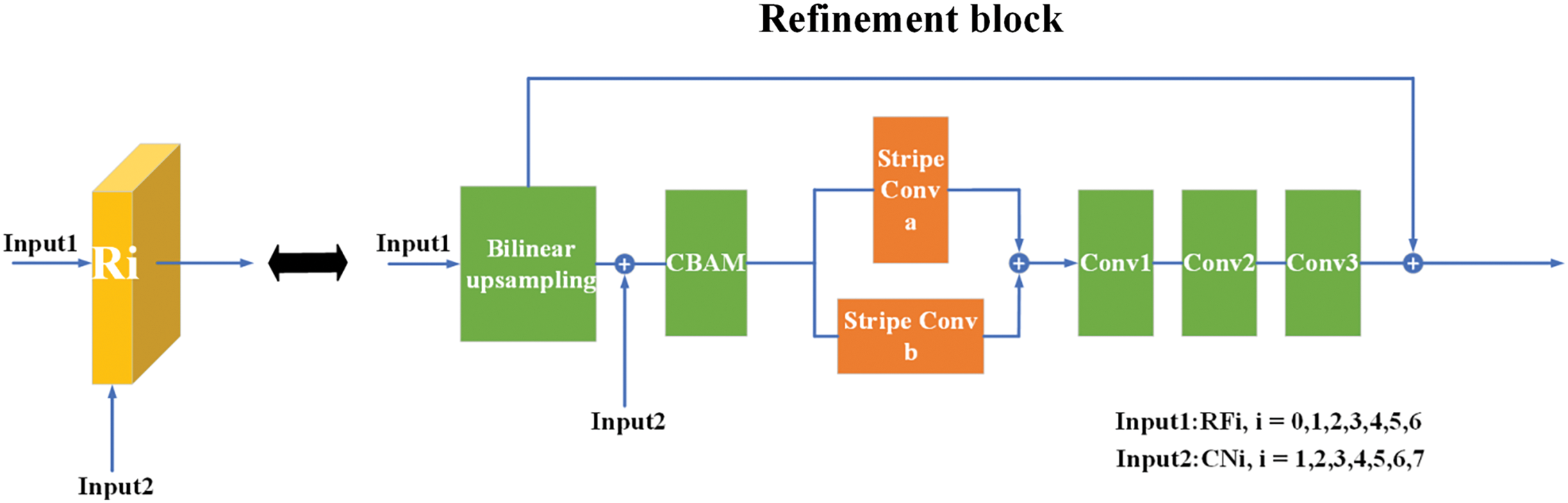
Figure 4: The structure of the edge-enhanced refinement module

4.2 CBAM Convolutional Block Attention Module

This article utilizes the CBAM convolutional attention mechanism [18], which combines channel attention and spatial attention, as a critical component of the edge-enhancing decoder. The primary objective of the CBAM attention mechanism is to enhance a convolutional neural network’s ability to perceive different feature channels and spatial locations, thereby improving the network’s performance. Specifically, CBAM’s channel attention module is able to learn the importance of each channel, obtain global information through global average pooling and global maximum pooling, and generate channel-level weights. This allows the network to more accurately focus on critical visual information, such as edges, corners, or textures, and suppress unimportant areas. The spatial attention module learns the weights of spatial positions based on the output of the channel attention module, so as to further emphasize the attention to important positions in the input feature map. This optimized feature representation not only improves the performance of the model, but also increases the generalization ability of the model, making it more robust to noise and irrelevant image content. By integrating CBAM into the depth prediction stage, motion estimation stage, and image reconstruction stage, the accuracy of depth estimation and the effect of edge enhancement can be improved, thereby improving the performance of the entire network in dynamic scenes.

The overall structure of CBAM, as shown in Fig. 5, involves taking an intermediate feature map as input and sequentially inferring attention maps along two independent dimensions—the channel dimension and the spatial dimension. These resultant attention maps are subsequently subjected to element-wise multiplication with the input feature map, thus executing adaptive feature modulation.

Figure 5: The overall structure of the Convolutional Attention Mechanism

For channel attention, as depicted in Fig. 6: In the first step, an input feature map of dimensions H×W×C is introduced, subsequently undergoing two parallel operations: global max-pooling (MaxPool) and global average-pooling (AvgPool) layers. These operations transform the feature map from a size of H×W×C to 1×1×C. In the second step, the feature map goes through a shared multi-layer perceptron (MLP) module, which compresses the number of channels to 1/r (r is the reduction ratio), and then expands it back to the original number of channels. Following this operation, ReLU activation is invoked, culminating in the generation of two activated features. Ultimately, by means of element-wise summation of the activated features and subsequent non-linear processing via a sigmoid activation function, the resultant outcome of channel attention is denoted as Mc∈Rc×1×1. The formulation is articulated as follows:

Mc(F)=σ(MLP(AvgPool(F))+MLP(MaxPool(F)))=σ(W1(W0(Favgc))+W1(W0(Fmaxc)))(4)

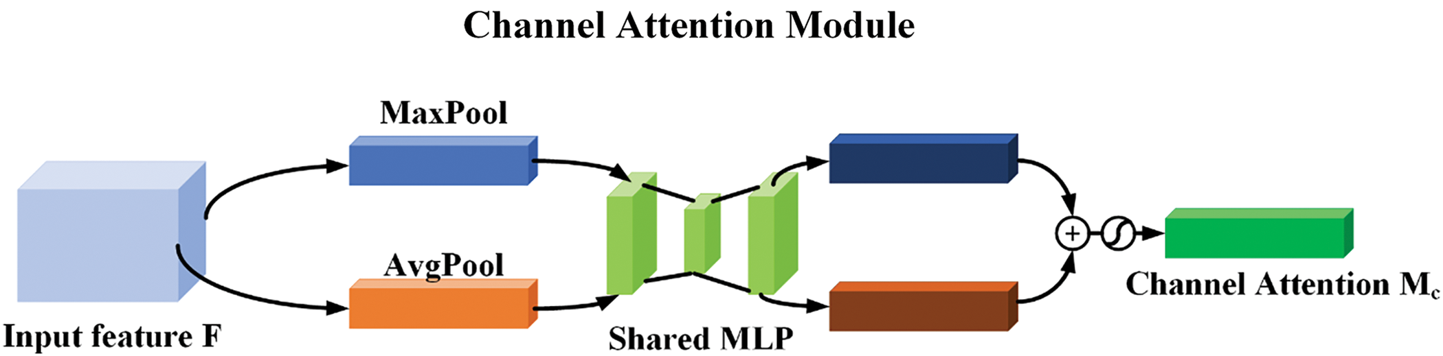
Figure 6: The channel attention mechanism structure

In this equation, σ represents the sigmoid activation function; W0∈RC×Cr represents the weights of the MLP; W1∈RCr×1×1 represents the weights of the ReLU activation function; Favgc and Fmaxc represent the global average pooling feature and global max pooling feature.

Concerning spatial attention, postulation is made for the feature map derived from channel attention, designated as F′, as depicted in Fig. 7. In the First step, the input feature map F′ sequentially undergoes MaxPool and AvgPool operations, yielding two feature maps of dimensions H×W×1 each. Subsequently, in the second step, the two obtained feature maps are concatenated and subjected to a 7×7 convolution operation to reduce the dimensionality to a solitary channel. Ultimately, the dimension-reduced features are passed through a sigmoid activation function, and the output is subjected to multiplication with the original image, thus restoring it to dimensions H×W×C. The output of spatial attention denominated as Ms∈RC×H×W. The formula for spatial attention can be expressed as:

Ms(F)=σ(f7×7([AvgPool(F);MaxPool(F)]))=σ(f7×7([Favgs;Fmaxs]))(5)

Figure 7: Structure of the spatial attention mechanism

In which, σ represents the sigmoid activation function, f denotes a convolution operation with a size of 7×7.

In summary, the entire CBAM convolutional attention mechanism process can be expressed using the following equations:

F′=Mc(F)⊗F(6)

F′′=MS(F)⊗F′(7)

where ⊗ represents element-wise multiplication. F′∈RC×1×1 represents the features obtained after applying channel attention. F′′∈RC×H×W is the final feature obtained after passing the intermediate feature F through the CBAM attention mechanism.

To illustrate the effectiveness of the edge enhancement module, we perform corresponding visualization experiments, as shown in Fig. 8a, first input RGB images; As discernible in Fig. 8b,c, post the traversal through the CBAM attention module, the decoder evinces a notable capability for delineating moving entities. Additionally, it contributes to the elucidation of the relative positional relationships between moving objects and the background, consequently yielding a reduction in artifacts and the augmentation of the clarity of edge information.

Figure 8: The visualization results of various components of the edge-enhanced module: (a) Input RGB image; (b) Initial feature extraction; (c) Features after CBAM; (d) Features after CBAM and stripe convolution

4.3 Stripe Convolution

Traditional convolutional kernels predominantly employ square configurations, whether in tasks about classification, semantic segmentation, or depth estimation. Such kernels only aggregate local features for each pixel and do not fully utilize boundary and global contextual features. Simultaneously, this conventional approach encumbers the neural network’s capacity to apprehend anisotropy, particularly when distinct objects exhibit relative motion against the background. As illustrated in Fig. 9, when considering two pedestrians on bicycles manifesting discretely within the scene, square convolution simplifies the convolutional kernel’s sampling process by encompassing nearby features that might be unrelated to the pedestrians. Consequently, upon weighted aggregation, this approach tends to engender indistinct and unclear delineations of the edges pertaining to moving objects within the predicted translation field. Contrastingly, as showcased in Fig. 10, stripe convolution is employed. This variant permits the utilization of strip-shaped convolutional kernels inherently biased toward specific orientations. Under the same convolution kernel size, stripe convolution has the characteristic to capture extensive spatial relationships, resulting in an expanded receptive field. Concurrently, it maintains a narrow kernel shape along other spatial dimensions, helping to connect contextual information during feature extraction from images and effectively preventing sampling interference in irrelevant areas.

Figure 9: Capture of moving objects by square convolution

Figure 10: Capture of moving objects by stripe convolution

Consequently, stripe convolution serves as an excellent complement to the conventional square convolution, aiding motion networks in extracting more detailed and discrete information about moving objects. In this study, stripe convolution was employed during the motion network’s decoding process to enhance the capture of discrete moving objects and extract information about the edges of these moving objects. The precise operational details of stripe convolution are delineated in Fig. 11, wherein a represents a 1 × 3 convolutional layer, and b represents a 3 × 1 convolutional layer. Convolution a aggregates pixels along the horizontal axis in proximity to the boundaries, while convolution b aggregates pixels vertically. Subsequent to these dual convolutional operations, an element-wise summation is executed to consolidate the features elicited by the two stripe convolutions. To ensure diversity in the fused features, no activation function is applied after stripe convolution. By virtue of stripe convolutions a and b effectively sampling global contextual information along orthogonal orientations, they impart pivotal cues for heightening the extraction of edge information pertaining to moving objects and the discerning of discrete moving objects. Thus, the application of this stripe convolution will fortify the discernment of edge and motion information for moving objects.

Figure 11: Details of stripe convolution

Notably, this enhancement is discernible in Fig. 8c,d, where the capacity to distinguish discrete objects, exemplified by the second-to-last car on the right side in image Fig. 8d, is markedly clearer. Additionally, the contours of the vehicles attain greater lucidity compared to image Fig. 8c, with a concurrent augmentation in the richness of edge detail information. Stripe Convolution is able to effectively capture the features of targets with different aspect ratios, especially for objects with high aspect ratios, where the geometry can be better extracted. This is especially important in dynamic scenes, where targets tend to have complex shapes and sizes. At the same time, because Stripe Convolution is more adaptable and flexible when dealing with elongated targets, it is able to capture the edge information of the target more accurately. This is a significant improvement for edge augmented networking frameworks, as it provides clearer and more accurate information at the edge, which improves the performance of the entire network.

Overall, in the unsupervised monocular depth estimation and edge enhancement networks of dynamic scenes, CBAM and strip convolutional modules enhance the depth estimation and edge enhancement capabilities of dynamic scenes through synergies. Specifically, CBAM first performs channel attention and spatial attention processing on input feature maps to enhance important features and suppress unimportant parts, while strip convolutional module captures target features with different aspect ratios to enhance feature extraction capabilities for high-aspect ratio targets and generate more comprehensive and accurate feature representations. In the motion estimation stage, CBAM optimizes the four-channel image containing depth information, and the strip convolution module extracts motion features to improve the accuracy of motion parameter estimation. In addition, the depth map and motion parameters optimized by CBAM are used to generate more accurate reconstructed images, and the strip convolution module further enhances the edge information, making the reconstructed images less different from the actual images, thus improving the training effect of the network.

5  Loss Function

In the realm of unsupervised deep learning for monocular cameras, the loss function assumes a paramount role and serves as the solitary source for imparting training supervision signals. In this paper, the loss function [16–18] primarily consists of four regularization components: (1) depth regularization Lreg,dep. (2) motion regularization Lreg,mot. (3) consistency regularization Lcyc. (4) edge enhancement regularization Ledge.

The objective of depth regularization resides in the regularization of depths within regions characterized by low gradients, explicated as follows:

Lreg,dep=αdep∬(|∂uD(u,v)|e−|∂uI(u,v)|+|∂vD(u,v)|e−|∂uI(u,v)|)dudv(8)

In this equation, αdep denotes a hyperparameter, D(u,v) represents the predicted depth map, I(u,v) represents the input RGB video frame, ∂D(u,v) represents the gradient of the image depths, and ∂I(u,v) represents the gradient of the image pixels.

Motion regularization is based on two properties of the residual translation field: (1) Sparsity, arising from the fact that most pixels in a frame typically belong to the background or static objects. (2) In 3D space, the shape of an entire rigidly moving object is often constant during translation. Consequently, motion regularization, denoted as Lreg,mot, imposed on the motion map T(u,v), incorporates two facets: group smoothing loss, denoted as Lg1, and sparsity loss, denoted as L1/2, elucidated as follows:

Lg1[T(u,v)]=∑i∈{x,y,z{}}∑∬(∂uTi(u,v))2+(∂uTi(u,v))2dudv(9)

where ∂T(u,v) represents the gradient of motion vectors in the motion field.

The sparsity loss, L1/2, is defined as:

L1/2[T(u,v)]=2∑i∈{x,y,z}⟨|Ti|⟩∬1+|Ti(u,v)|⟨|Ti|⟩dudv(10)

where ⟨|Ti|⟩ is the spatial average of |Ti(u,v)||Ti(u,v)|, and this regularization is self-normalized. The final motion regularization loss expressed as:

Lreg,mot=αmotLg1[Tobj(u,v)]+βmotL1/2[Tobj(u,v)](11)

The Consistency regularization consists of two components: motion cycle consistency loss, denoted as Lcyc and occlusion and photometric consistency loss, denoted as Lrgb. Lcyc encourages the forward and backward motions between any pair of frames to be opposite to each other:

Lcyc=αcyc‖RRinv−1‖‖RR−1‖2+‖RRinv−1‖2+βcyc∬‖RinvT(u,v)+Tinv(uwarp,vwarp)‖‖T(u,v)‖2+‖Tinv(uwarp,vwarp)‖2dudv(12)

where the subscript ‘inv’ indicates the same quantity obtained when the input frames are reversed in order, and the subscript ‘warp’ indicates the warp operation. αcyc and βcyc represent hyperparameters. Lrgb encourages photometric consistency, including L1 loss in RGB space and SSIM loss:

Lrgb=αrgb∬|I(u,v)−Iwarp(u,v)|D(u,v)>Dwarp(u,v)dudv+βrgb1−SSIM(I,Iwarp)2(13)

where I and Iwarp are the original image and the reconstructed image, respectively.

The first three regularization components closely align with prior research, while in this study we introduce a novel regularization termed edge regularization. Edge regularization is an improvement based on the Laplacian operator and possesses rotation invariance. It can identify edge strength and direction using image gradients. For the predicted residual translation field, edge regularization can effectively capture the edge intensity of moving objects and accelerate the convergence speed of the neural network. The formula is expressed as follows:

Ledge[T(u,v)]=∑i∈{x,y,z{}}∑∬(∂2Ti(u,v)∂2u2)2+(∂2Ti(u,v)∂2v2)2dudv(14)

where ∂2T(u,v) represents the variation in the gradient of motion vectors in the motion field.

In summation, the composite loss function for the entire network is articulated as follows:

Ltotal=Lreg,mot(Lg1(groupsmoothnessloss)+L12(sparsityloss))+Lreg,depth+Lcyc(rotation+translation)+Lrgb(rgb_consistency+ssim)+Ledge(15)

6  Experiments

6.1 KITTI Dataset and Cityscapes Dataset

The KITTI dataset stands as a classic corpus in the realm of autonomous driving and computer vision endeavors. It encompasses a multitude of images representing diverse scenarios, including highways, urban locales, and residential areas. In the context of our investigation, we harnessed a set of 22,600 image pairs from the KITTI dataset for training purposes, and an additional 697 image pairs were allocated for assessing the performance of our experimental models. In a distinctive vein, the Cityscapes dataset emerges as a more formidable benchmark, particularly tailored to the domain of autonomous driving within dynamic urban environments. Unlike the KITTI dataset, Cityscapes is meticulously crafted to cater specifically to autonomous driving challenges within urban settings. In our research, we made use of 22,973 image pairs derived from a summation of high-quality annotated and roughly annotated images, capitalizing on them for the training process. We applied the same evaluation methodology as employed in previous experiments. Due to the absence of a standard evaluation protocol for the Cityscapes dataset, we solely applied the evaluation method from the Cityscapes dataset to our ablation experiments.

6.2 Implementation Details

In this paper, the complete network architecture was instantiated utilizing the TensorFlow framework, and the model underwent training on an NVIDIA GeForce RTX 3070. The training process of unsupervised monocular depth estimation and edge enhancement network for dynamic scenes is mainly as follows: firstly, the image sequence dataset containing dynamic scenes is selected and preprocessed and data augmented. Then, initialize the network parameters and define the loss function. During the training process, depth prediction (extracting features and estimating depth maps), motion estimation (calculating optical flow and optimization), and image reconstruction (generating intermediate images and enhancing edges) are performed sequentially, and the training is optimized through learning rate adjustment, regularization, and batch normalization. Thereinto, the deep prediction network and the motion estimation network were trained for 106 iterations using the Adam optimizer with a learning rate set to 104. The training batch size was set to 16, and the training RGB images had a resolution of 1248×128. The settings of several hyperparameters in the loss function: In Eq. (8), αdep is set to 10−3. In Eq. (11), αmot is set to 1.0, and βmot is set to 0.2. In Eq. (12), αcyc is set to 10−3, and βcyc is set to 5×10−2. In Eq. (13), αrgb is set to 1.0, and βrgb is set to 0.8.

6.3 Evaluation Metrics

Building upon Zhou’s [20] prior work, this paper cites five standard evaluation metrics and compares accuracy and error against state-of-the-art methods on these five metrics. These metrics include: root mean square error (RMSE), square relative error (Sq Rel), root mean square logarithmic error (RMSE log), absolute relative error (Abs Rel), and threshold accuracy (δi, ii = 1, 2, 3). Each metric is calculated as follows:

δi=max(ypredygt,ygtypred)<thr(16)

Abs Rel=1n∑pn|ypred−ygt|ypred(17)

Sq Rel=1n∑pn|ypred−ygt|2ypred(18)

RMSE=1n∑pn(ypred−ygt)2(19)

RMSElog=1n∑pn|log(ypred)−log(ygt)|2(20)

In the equation, ypred represents the predicted depth value for a pixel, ygt represents the true or ground truth depth value for the same pixel, and n represents the total number of pixels for which true depth values are available in the ground truth depth map.

6.4 Analysis of the Experimental Results

To demonstrate the effectiveness and superiority of the proposed improvement method in this paper, a series of experiments were conducted on both the KITTI dataset and the Cityscapes dataset, comparing the experimental results of this paper’s method with other unsupervised monocular depth estimation methods. The quantitative results are summarized in Table 1, while the qualitative results are visually depicted in Fig. 12. In the column labeled Motion Model, “√” means that a motion model is used, and “×” means that a motion model is not used. The bold annotation indicates the optimal results of each evaluation metric when using the motion model. For the red metrics, lower is better; for the green metrics, higher is better.

Figure 12: Qualitative results analysis of selected methods corresponding to Table 1 on the KITTI dataset

From Table 1, the following observations can be made: (1) When motion models are used, our proposed method consistently shows significant improvements over the optimal method across different resolutions. Specifically, our model demonstrates reductions of no less than 8% in absolute relative error, 15% in square relative error, and 2% in root mean square error compared to the best method. (2) At equivalent resolutions, when compared to the optimal method without using a motion model, our proposed model exhibits decrease of 4% in absolute relative error, 4% in square relative error, and 3% in root mean square error relative to the best. (3) Under the same resolution and both using motion models, our proposed model shows a reduction of 7% in absolute relative error, a decrease of 4% in square relative error, and a decrease of 7% in root mean square error compared to the best method. (4) Compared with the latest monocular depth estimation methods SDFA-Net [32], CATNet [33], PrimeDepth [34] and MonoProb [35], the proposed method still achieves the best in multiple indicators, which shows the effectiveness of each module proposed in this paper.

To visually demonstrate the comparative effectiveness of our model against other models, we have replicated a subset of the models from Table 1 and compared them with our method, as shown in Fig. 12. Within Fig. 12, ‘Raw’ represents the original test image, while ‘Zhou et al. [20]’, ‘GeoNet [22]’, ‘DDVO [28]’, ‘Yang et al. [30]’, and ‘Li [25]’ correspond to the depth maps predicted by the models listed in Table 1. Regions of particular interest enclosed by red circles are emphasized for observation. In the second column test image (from left to right), we pay special attention to the area in front of the house, specifically the part with the large tree. Our model’s predictions can clearly capture the trunk of the large tree and distinguish it from the adjacent billboard pole. In contrast, the distinctions made by other models appear less clear and more ambiguous. In the fourth column test image (from left to right), near the car, we can see a triangular road sign. Our predicted depth map accurately captures the edges and contours of the triangular road sign, while other test models either cannot distinguish the road sign’s outline or produce a more blurred representation. Therefore, both qualitative and quantitative test results indicate that our proposed method outperforms previous methods in terms of depth estimation quality across different resolutions and whether or not a motion model is applied.

6.5 Ablation Experiment

To validate the effectiveness of the edge-enhanced decoder proposed in this paper for improving depth prediction capability, taking a resolution of 128 × 416 as an example, comparative ablation experiments were conducted to analyze the impact of the main components of the edge-enhanced decoder, which include the CBAM attention module and the stripe convolution module, on the prediction results. At the same time, we also analyze the impact of edge regularization loss on the performance of the model proposed in this paper.

(1) Effectiveness analysis of CBAM attention module and strip convolution module

By adding stripe convolution to the baseline, the network takes better advantage of boundary and global contextual features, resulting in an enhanced capture of discrete moving objects. As seen in Table 2, the network shows improved accuracy as a result. Among them, the absolute relative Error, square relative error, and root mean square error have reduced by 3%, 3%, and 8%, respectively. After adding the CBAM attention module to the baseline, the network’s perception capability for different feature channels and spatial positions is enhanced. Additionally, it improves the segmentation of moving objects within the motion network and clarifies the spatial relationship between moving objects and the background. As shown in Table 2, there is a slight improvement in accuracy as well. Among them, the absolute relative error, square relative error, and root mean square error have reduced by 7%, 2%, and 6%, respectively, after adding the CBAM attention module to the baseline. If both stripe convolution and CBAM attention modules are used on top of the baseline, the network’s ability to extract and integrate edge information is maximized. This can be qualitatively described as follows in Fig. 13: (1) Test the image on the first line, we can observe that the baseline depth map does not clearly capture the pedestrian walking in the middle. However, when using stripe convolution and the CBAM attention module, our depth map can capture the pedestrian in the middle. (2) Test the images on the third, fourth, and fifth line, there are holes in the depth maps generated by the baseline to describe vehicles. But with the addition of stripe convolution and CBAM attention modules, our depth map is smoother. (3) In these five lines all test images, the baseline predicts blurred edges for moving objects in the motion field. Additionally, some images exhibit edge omissions, such as the fifth test image. Conversely, with the inclusion of stripe convolution and CBAM attention modules, the contours of moving objects in our motion field are clearer, and edge omissions are not present. Based on the analysis of Table 2, it can be observed that adding stripe convolution and the CBAM attention module to the baseline has led to an reduce in the absolute relative error, square relative error, root mean square error, and root mean square logarithmic error by 9%, 4%, 7%, and 1%, respectively. Lastly, as shown in Table 3, it can be observed that the selected 1 × 3 stripe convolution in this paper can maximize the utilization of boundary information and fully harness the potential of stripe convolution to its fullest extent.

Figure 13: Qualitative analysis of using an edge-enhanced decoder vs. Not using an edge-enhanced decoder on the cityscapes dataset

The ablation experiments demonstrate that each component of the edge-enhanced decoder in this paper contributes effectively to improving the network’s accuracy, and the best results are achieved when both components are combined.

(2) Effectiveness analysis of edge regularization method

In order to verify the effectiveness of the edge regularization proposed in this paper, we also carried out the corresponding ablation experiment analysis, and analyzed the convergence of the overall network by analyzing the change of rotation and translation scale factors with the increase of training steps to evaluate its performance. Specifically, when applying depth regularization, motion regularization, consistency regularization, and subsequently adding edge regularization atop the initial three, accompanied by an increase in training iterations (epochs) and variations in rotation and translation scale factors, as illustrated in Fig. 14a,b. Both for rotational scale factors and translational scale factors, after adding edge regularization, both the rotational and translational scale factors converge after approximately 550 k steps, while without adding edge regularization, both the rotational and translational scale factors converge after about 770 k steps, resulting in a 28% increase in convergence speed when edge regularization is applied. At the same time, the motion network without edge regularization tends to experience a sharp increase in gradients around 550 k steps. With the addition of edge regularization, gradient changes become more uniform, leading to smoother network learning and better convergence results.

Figure 14: The changes in scale factors of the motion network during the training process. Among them, (a) represents the change of the rotation scale factor before and after the regularization of the network is added in the training process, and (b) represents the change of the translation scale factor before and after the regularization of the network is added in the training process

7  Conclusions

In view of the challenge of monocular depth estimation in dynamic scenes, this paper proposes an edge-enhanced unsupervised monocular depth estimation algorithm for dynamic scenes, which solves the current problems of edge blurring and difficult capture of moving objects in dynamic scenes. By designing an edge-enhanced decoder and a new edge loss function, the performance of the model when dealing with dynamic targets is effectively improved. The edge-enhanced decoder uses the CBAM module and strip convolution technology to enhance the ability to capture the edge features of moving objects. At the same time, the edge loss function based on the Laplace operator accelerates the convergence of the model and avoids the gradient explosion problem. Experiments on KITTI and Cityscapes datasets show that compared with the existing technologies, the proposed method has a significant improvement in depth estimation accuracy, with an RMSE reduction of 4.8% and a 36% increase in model convergence speed. These results show that the proposed method has obvious advantages in the fine processing of depth map edges and the accurate capture of moving targets in dynamic scenes, which effectively enhances the prediction ability of the network on the edge region and provides an effective technical solution for the depth perception of autonomous vehicles.

Acknowledgement: Thanks to the editor and anonymous reviewer for their insightful comments, which have improved the quality of this publication.

Funding Statement: This research was funded by the Yangtze River Delta Science and Technology Innovation Community Joint Research Project (2023CSJGG1600), the Natural Science Foundation of Anhui Province (2208085MF173) and Wuhu “ChiZhu Light” Major Science and Technology Project (2023ZD01, 2023ZD03).

Author Contributions: The authors confirm contribution to the paper as follows: Conceptualization, data curation, funding acquisition, project administration: Peicheng Shi; conceptualization, writing—editing: Yueyue Tang; investigation, methodology, visualization, writing—original draft: Yi Li; methodology, visualization, review, revise: Xinlong Dong; resources, supervision, validation: Yu Sun; writing—review & editing: Aixi Yang. All authors reviewed the results and approved the final version of the manuscript.

Availability of Data and Materials: The authors confirm that the data supporting the findings of this study are available within the article.

Ethics Approval: Not applicable.

Conflicts of Interest: The authors declare no conflicts of interest to report regarding the present study.

References

1. Zou L, Hu L, Wang Y, Wu Z, Wang X. Perpendicular-cutdepth: perpendicular direction depth cutting data augmentation method. Comput Mater Contin. 2024;79(1):927. doi:10.32604/cmc.2024.048889. [Google Scholar] [CrossRef]

2. Dong X, Shi P, Qi H, Yang A, Liang T. TS-BEV: BEV object detection algorithm based on temporal-spatial feature fusion. Displays. 2024;84(1–2):102814. doi:10.1016/j.displa.2024.102814. [Google Scholar] [CrossRef]

3. Wang H, Shi Z, Zhu C. Enhanced multi-scale object detection algorithm for foggy traffic scenarios. Comput Mater Contin. 2025;82(2):2451. doi:10.32604/cmc.2024.058474. [Google Scholar] [CrossRef]

4. Yin Y, Zhang L, Shi X, Wang Y, Peng J, Zou J. Improved double deep Q network algorithm based on average Q-value estimation and reward redistribution for robot path planning. Comput Mater Contin. 2024;81(2):2769. doi:10.32604/cmc.2024.056791. [Google Scholar] [CrossRef]

5. Islam QU, Ibrahim H, Chin PK, Lim K, Abdullah MZ. MVS-SLAM: enhanced multiview geometry for improved semantic RGBD SLAM in dynamic environment. J Field Robot. 2024;41(1):109–30. doi:10.1002/rob.22248. [Google Scholar] [CrossRef]

6. Islam QU, Khozaei F, Baig I, Ignatyev D. Advancing autonomous SLAM systems: integrating YOLO object detection and enhanced loop closure techniques for robust environment map. Robot Auton Syst. 2025;185(4):104871. doi:10.1016/j.robot.2024.104871. [Google Scholar] [CrossRef]

7. Islam QU, Ibrahim H, Chin PK, Lim K, Abdullah MZ, Khozaei F. ARD-SLAM: accurate and robust dynamic SLAM using dynamic object identification and improved multi-view geometrical approaches. Displays. 2024;82(9):102654. doi:10.1016/j.displa.2024.102654. [Google Scholar] [CrossRef]

8. Li H, Ma Y, Gu Y, Hu K, Liu Y, Zuo X. RadarCam-Depth: radar-camera fusion for depth estimation with learned metric scale. In: Proceedings of the 2024 IEEE International Conference on Robotics and Automation (ICRA); 2014 May 13–17; Yokohama, Japan. Piscataway, NJ, USA: IEEE; 2024. p. 10665–72. [Google Scholar]

9. Li A, Hu A, Xi W, Yu W, Zou D. Stereo-lidar depth estimation with deformable propagation and learned disparity-depth conversion. In: Proceedings of the 2024 IEEE International Conference on Robotics and Automation (ICRA); 2024 May 13–17; Yokohama, Japan. Piscataway, NJ, USA: IEEE; 2024. p. 2729–36. [Google Scholar]

10. Song M, Lim S, Kim W. Monocular depth estimation using laplacian pyramid-based depth residuals. IEEE Trans Circuits Syst Video Technol. 2021;31(11):4381–93. doi:10.1109/tcsvt.2021.3049869. [Google Scholar] [CrossRef]

11. Fu H, Gong M, Wang C, Batmanghelich K, Tao D. Deep ordinal regression network for monocular depth estimation. In: Proceedings of the IEEE Conference on Computer Vision and Pattern Recognition; 2018 Jun 18–23; Salt Lake, UT, USA. Piscataway, NJ, USA: IEEE Press; 2018. p. 2002–11. [Google Scholar]

12. Yang M, Yu K, Zhang C, Li Z, Yang K. Denseaspp for semantic segmentation in street scenes. In: Proceedings of the IEEE Conference on Computer Vision and Pattern Recognition; 2018 Jun 18–23; Salt Lake, UT, USA. Piscataway, NJ, USA: IEEE Press; 2018. p. 3684–92. [Google Scholar]

13. Godard C, Mac Aodha O, Brostoe GJ. Unsupervised monocular depth estimation with left-right consistency. In: Proceedings of the IEEE Conference on Computer Vision and Pattern Recognition; 2017 Jul 21–26; Honolulu, HI, USA. Piscataway, NJ, USA: IEEE Press; 2017. p. 270–9. [Google Scholar]

14. Lee S, Im S, Lin S, Kweon IS. Learning monocular depth in dynamic scenes via instance aware projection consistency. In: Proceedings of the AAAI Conference on Artificial Intelligence; 2021 May 19–21; AAAI Press. p. 1863–72. [Google Scholar]

15. Gordon A, Li H, Jonschkowski R, Angelova A. Depth from videos in the wild: unsupervised monocular depth learning from unknown cameras. In: Proceedings of the IEEE/CVF International Conference on Computer Vision; 2019 Oct 27–Nov 2; Seoul, Republic of Korea. p. 8977–86. [Google Scholar]

16. Casser V, Pirk S, Mahjourian R, Angelova A. Depth prediction without the sensors: leveraging structure for unsupervised learning from monocular videos. In: Proceedings of the AAAI Conference on Artificial Intelligence; 2019 Jan 27–Feb 1; Honolulu, HI, USA. p. 8001–8. [Google Scholar]

17. Sun Y, Hariharan B. Dynamo-depth: fixing unsupervised depth estimation for dynamical scenes. Adv Neural Inf Process Syst. 2023;36:54987–5005. [Google Scholar]

18. Woo S, Park J, Lee JY, Kweon IS. CBAM: convolutional block attention module. In: Proceedings of the EuropeanConference on Computer Vision (ECCV); 2018 Sep 8–14; Munich, Germany. p. 3–19. [Google Scholar]

19. Garg R, Bg VK, Carneiro G, Reid I. Unsupervised CNN for single view depth estimation: geometry to the rescue. In: Proceedings of the European Conference on Computer Vision; 2016 Oct 11–14; Amsterdam, The Netherlands. Cham, Switzerland: Springer; 2016. p. 740–56. [Google Scholar]

20. Zhou T, Brown M, Snavely N, Lowe DG. Unsupervised learning of depth and ego-motion from video. In: Proceedings of the IEEE Conference on Computer Vision and Pattern Recognition; 2017 Jul 21–26; Honolulu, HI, USA. p. 1851–8. [Google Scholar]

21. Godard C, Mac Aodha O, Firman M, Brostow GJ. Digging into self-supervised monocular depth estimation. In: Proceedings of the IEEE/CVF International Conference on Computer Vision; 2019 Oct 27–Nov 2; Seoul, Republic of Korea. p. 3828–38. [Google Scholar]

22. Yin Z, Shi J. GeoNet: unsupervised learning of dense depth, optical flow and camera pose. In: Proceedings of the IEEE Conference on Computer Vision and Pattern Recognition; 2018 Jun 18–23; Salt Lake, UT, USA. p. 1983–92. [Google Scholar]

23. Luo C, Yang Z, Wang P, Wang Y, Xu W, Nevatia R, et al. Every pixel counts++: joint learning of geometry and motion with 3D holistic understanding. IEEE Trans Pattern Anal Mach Intell. 2019;42(10):2624–41. doi:10.1109/tpami.2019.2930258. [Google Scholar] [PubMed] [CrossRef]

24. Casser V, Pirk S, Mahjourian R, Angelova A. Unsupervised monocular depth and ego-motion learning with structure and semantics. In: Proceedings of the IEEE/CVF Conference on Computer Vision and Pattern Recognition Workshops; 2019 Jun 16–17; Long Beach, CA, USA. p. 1–8. [Google Scholar]

25. Li H, Gordon A, Zhao H, Casser V, Angelova A. Unsupervised monocular depth learning in dynamic scenes. In: Proceedings of the Conference on Robot Learning; 2021 Nov 8–11; London, UK. p. 1908–17. [Google Scholar]

26. Jing J, Liu S, Wang G, Zhang W, Sun C. Recent advances on image edge detection: a comprehensive review. Neurocomputing. 2022;503:259–71. doi:10.1016/j.neucom.2022.06.083. [Google Scholar] [CrossRef]

27. Huang G, Bors AG. Busy-quiet video disentangling for video classification. In: Proceedings of the IEEE/CVF Winter Conference on Applications of Computer Vision; 2022 Jan 3–8; Waikoloa, HI, USA. p. 1341–50. [Google Scholar]

28. Wang C, Buenaposada JM, Zhu R, Lucey S. Learning depth from monocular videos using direct methods. In: Proceedings of the IEEE Conference on Computer Vision and Pattern Recognition; 2018 Jun 18–23; Salt Lake, UT, USA. p. 2022–30. [Google Scholar]

29. Ranjan A, Jampani V, Balles L, Kim K, Sun D, Wulff J, et al. Competitive collaboration: joint unsupervised learning of depth, camera motion, optical flow and motion segmentation. In: Proceedings of the IEEE/CVF Conference on Computer Vision and Pattern Recognition; 2019 Jun 15–20; Long Beach, CA, USA. p. 12240–9. [Google Scholar]

30. Yang Z, Wang P, Wang Y, Xu W, Nevatia R. Every pixel counts: unsupervised geometry learning with holistic 3d motion understanding. In: Proceedings of the European Conference on Computer Vision (ECCV) Workshops; 2018 Sep 8–14; Munich, Germany. [Google Scholar]

31. Luo X, Huang JB, Szeliski R, Matzen K, Kopf J. Consistent video depth estimation. ACM Trans Graph. 2020;39(4):71. doi:10.1145/3386569.3392377. [Google Scholar] [CrossRef]

32. Zhou Z, Dong Q. Self-distilled feature aggregation for self-supervised monocular depth estimation. In: Proceedings of the European Conference on Computer Vision; 2022 Oct 23–27; Tel Aviv, Israel. Cham, Switzerland: Springer Nature; 2022. p. 709–26. [Google Scholar]

33. Tang S, Lu T, Liu X, Zhou H, Zhang Y. CATNet: convolutional attention and transformer for monocular depth estimation. Pattern Recognit. 2024;145(17):109982. doi:10.1016/j.patcog.2023.109982. [Google Scholar] [CrossRef]

34. Zavadski D, Kalšan D, Rother C. PrimeDepth: efficient monocular depth estimation with a stable diffusion preimage. In: Proceedings of the Asian Conference on Computer Vision; 2024 Dec 8–12; Hanoi, Vietnam. p. 922–40. [Google Scholar]

35. Marsal R, Chabot F, Loesch A, Grolleau W, Sahbi H. MonoProb: self-supervised monocular depth estimation with interpretable uncertainty. In: Proceedings of the IEEE/CVF Winter Conference on Applications of Computer Vision; 2024 Jan 3–8; Waikoloa, HI, USA. p. 3637–46. [Google Scholar]