DeblurTomo: Self-Supervised Computed Tomography Reconstruction from Blurry Images

1  Introduction

Computed tomography (CT) reconstruction is a technology that converts X-ray projection data from multiple angles into a 3D image and visualizes the internal structure of objects and is widely used in medical diagnosis [1,2] and materials science [3]. High-resolution CT images are crucial in these fields, such as in distinguishing small lesions in medical diagnosis.

However, high-quality CT reconstruction highly depends on sharp and clear X-ray projections. The resolution of these projections is primarily affected by two main factors: the source blur caused by the excessively large ray source aperture [4,5] and the scattering blur caused by ray scattering [6]. Reconstruction algorithms that assume point sources and no scattering can lead to artifacts in CT images. Upgrading imaging equipment with ray sources of smaller size and higher energy can achieve more precise results. However, the high cost generally limits the available scenarios.

The most commonly used deblurring method is to restore the image in the projection domain, estimate the blur kernel of the projection image by measurement and calculation [9–11], and then perform deconvolution to restore the clear projection image [12,13]. Nevertheless, the measurement process is cumbersome and not always feasible. Another method is to model the system blur based on its principles and incorporate it into the iterative reconstruction algorithm without the need for the blur measurement process [14–16]. However, these methods do not consider the variation of system blur at different object positions and distance from detectors in the imaging depth direction [17], and the discrete representation of the iterative reconstruction algorithm is inconsistent with the continuous reconstruction object, which easily leads to artifacts [18]. Recently, much research has been done on deep-learning image restoration algorithms [17,19]. Still, due to the general lack of dataset diversity, the generalization performance of such work cannot meet the needs of complex CT reconstruction scenarios. Therefore, it is essential to construct a reconstruction algorithm that can incorporate spatial information for blur modeling and reconstruct clear CT images without relying on measurements and external datasets.

This work tries to solve the above problem using Implicit Neural Representation (INR) [20]. INR has three characteristics: (a) INR uses neural networks to represent space as a continuous function, generating corresponding physical properties (e.g., attenuation coefficients) at arbitrary coordinates without being limited by resolution and can better fit continuous reconstruction scenes. (b) As a natural self-supervised method, INR can complete reconstruction using only projection images, without external datasets. (c) Neural networks in INR contain rich geometric information, which helps the model integrate relevant information between blur and spatial. Based on the above characteristics, we believe that INR is suitable for solving the problem of blur reconstruction. However, incorporating spatial information for blur modeling and solving the long training time are still challenging.

This paper proposes DeblurTomo, a self-supervised implicit neural representation-based deblurring reconstruction algorithm, introducing INR into CT reconstruction deblurring for the first time. Specifically, we construct a reconstruction network by combining a multiresolution hash encoder and a multilayer perceptron (MLP), significantly reducing the training time. Moreover, we model the projection blur in 3D space and design a Ray Correction Network (RCN) and Weight Proposal Network (WPN) to generate corrected rays by integrating multi-view and spatial information to approximate the blurring process. The corrected rays have high flexibility, but they tend to bring distortion to both the corrected rays and the 3D scene simultaneously. We propose constraint loss by constraining one of the corrected rays near the assumed ray, preserving its flexibility while preventing unexpected offsets in the corrected rays. Extensive experiments on several datasets demonstrate the effectiveness of the proposed method, as shown in Fig. 1 and Section 4. Contributions are summarized as follows:

•   We propose a novel framework to reconstruct high-quality CT images from blurry inputs.

•   We propose the ray correction and weight proposal networks, which can effectively approximate various types of physical blurring processes and extend 2D deblurring to 3D space.

•   Extensive evaluations are conducted under multiple challenging real and synthetic datasets(blurry, noisy, sparse view and limited angle), demonstrating the effectiveness of the proposed method.

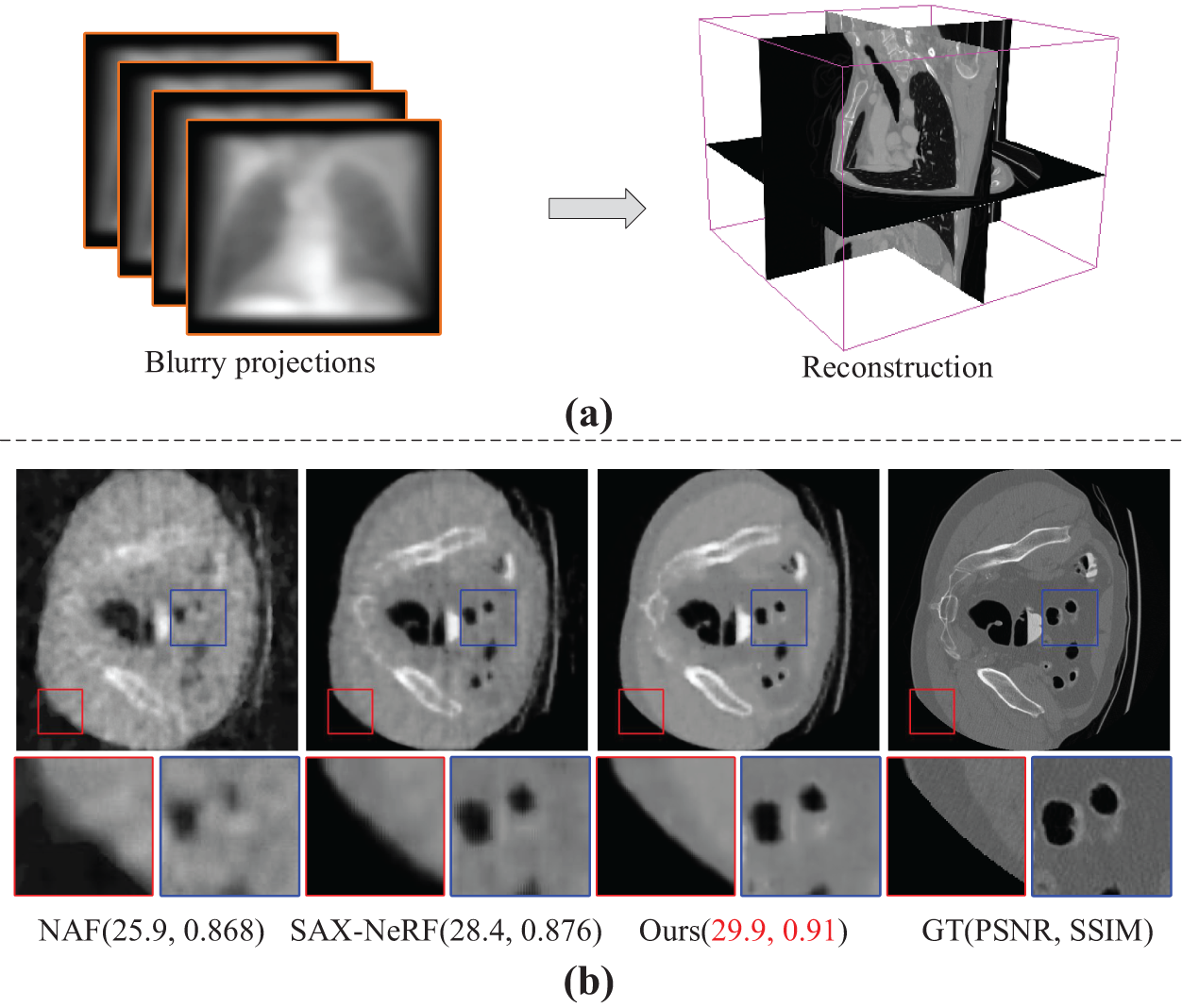
Figure 1: (a) The attenuation coefficient distribution of the 3D scene is reconstructed by using the multi-view blurry projections as input. (b) Comparison of reconstruction quality with other SOTA methods. The proposed method has fewer artifacts and richer reconstruction details, far surpassing NAF [7] and SAX-NeRF [8] in terms of PSNR and SSIM metrics

2  Related Work

2.1 Traditional Computed Tomography

The analytical method is the most commonly used reconstruction algorithm, which reconstructs the projection data by filtering and back-projecting. The typical representative is the (Filtered Back-Projection) FBP proposed by Feldkamp et al. [21] and its 3D cone beam variant FDK, which has the advantages of fast reconstruction speed, but it is difficult to handle highly ill-posed problems such as sparse-view and limited-angle.

Iterative algorithms usually use iterative optimization to minimize the difference between measured and predicted data [22], and can also combine regularization terms to optimize the iterative framework. Iterative reconstruction algorithms have shown promising results in sparse-view [23,24] and limited angles [25,26] imaging, but these methods suffer from the drawback of complex hyperparameter tuning, and their discrete representation methods are prone to artifacts [18].

In practical applications, in addition to medical diagnosis and industrial detection, a novel cultural heritage representation form is designed by combining 3D imaging and tomography [27,28].

2.2 Blur Reduction in Computed Tomography

CT image blur restoration methods can be divided into projection domain deconvolution, iterative image deblurring, and deep learning.

The projection domain deconvolution method directly deblurring the projection image, which calculates the projection image blur kernel through measurement [10,11], and then performs deconvolution [5,12,13]. Joshi et al. [10] utilized the sharp edges of objects in the image for blur estimation. Mohan [11] estimated blur from X-ray images of tungsten plates with sharp edges, modeled the blur as a convolution of multiple blur kernels and proposed a deconvolution method. However, blur measurements are not always feasible. Although blind deconvolution [29] can avoid blur measurement, it is also easy to amplify noise and cause artifacts.

The iterative image deblurring methods model the system blur and incorporate it into the iterative reconstruction algorithm. Tilley et al. [14] modeled the blur based on the iterative method of statistical model and performed the deblurring reconstruction by regularization and least-squares method. Reference [15] utilized the correlation between blur and noise for modeling, combined with the Gaussian likelihood objective function for reconstruction. Reference [16] modeled the Shift-Variant focal spot blur and incorporated it into the model-based iterative reconstruction algorithm, which achieved better results than the reconstruction algorithm without considering blur. However, these methods do not consider the changes in system blur at different object positions and distances from the detector in the imaging depth direction [17].

Deep learning methods usually use super-resolution (SR) techniques for deblurring in the image domain [30–32], but it is challenging to obtain datasets and cannot be used in unknown scenes [33]. We believe that a deblurring reconstruction algorithm suitable for arbitrary scenes is necessary.

2.3 Implicit Neural Representations

In the field of 3D vision, scenes are usually represented by discrete methods (voxels, pixels, and point clouds). NeRF proposed by Mildenhall et al. [20] uses a neural network (usually an MLP) to represent the scene as a function that maps coordinates to physical properties of interest (color, density, etc.). Compared with discrete representation methods, this representation method is continuous and more accurately represents the continuous physical world. Subsequent work has refined NeRF in detail [34,35] and expanded its applications [36], further demonstrating the superiority of INR.

In CT reconstruction, INR can alleviate the artifacts produced by discrete representation in traditional iterative reconstruction [18]. Unlike NeRF, INR in CT reconstruction only needs to learn a mapping function from coordinates to attenuation coefficients and does not require color and perspective information. Moreover, CT focuses more on the entire reconstructed space than surface information. Therefore, there are still many challenges in using INR for CT reconstruction [37]. Zha et al. [7] and Rückert et al. [38] combined voxel grid representation to reduce reconstruction time and improve accuracy. SAX-NeRF [8] utilized the Transformer to capture the intrinsic relationship of spatial structure. However, none of these methods consider the blur problem in CT imaging.

The INR deblurring modeling method in natural scenes [34] has been inspiring to us, but it does not account for ray scattering. We model the principle of blur in CT imaging systems and combine spatial depth information and geometric information for blur correction. To our knowledge, the proposed Deblurtomo is the first to use INR for deblurring reconstruction.

3  Method

CT blur arises from discrepancies between actual and assumed ray paths, and we aim to correct this for accurate reconstruction. We optimize the assumed rays and obtain multiple corrected rays to fit the real rays. The specific scheme is shown in Fig. 2. First, we construct a self-supervised implicit representation reconstruction algorithm as the basic scheme for reconstruction (see Section 3.2). Then, we propose the Ray Correction Network (RCN) and the Weight Proposal Network (WPN) to optimize the assumed ray, obtaining multiple corrected rays and their corresponding weights to fit the real blurring process (see Sections 3.3 and 3.4). Finally, the corrected rays are rendered using the reconstruction network, and weighted sums are performed to obtain the predicted blurry projection values supervised by measurement projection images (see Section 3.5).

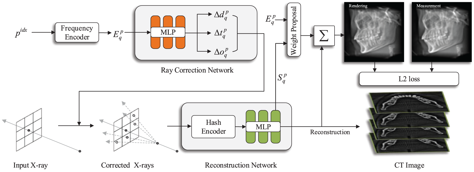
Figure 2: Overview of DeblurTomo pipeline. The ray correction network calculates multiple corrected rays via the encoding Eqp of the pixel index value (pidx). The weight proposal network utilizes Eqp, and depth features Sqp to generate weights for corrected rays. The reconstruction network integrates and renders the corrected rays and performs a weighted sum to obtain the final rendered projection image. During the reconstruction phase, it only needs to query the corresponding attenuation coefficient of the spatial coordinates in the reconstruction network to obtain the corrected CT image

3.1 Problem Formulation

The principle of X-ray imaging is the key to formulating the reconstruction problem. The X-ray passes through the target object and attenuates, and the detector measures the attenuated X-ray to obtain a 2D projection image. According to Beer’s law [39], the attenuation of rays is related to the thickness of the object and the attenuation coefficient, and the continuous form can be expressed as:

I^(p)I^0(p)=exp⁡(−∫tntfμ(rp(t))dt),(1)

where I^(p) is the projection value of the pixel coordinate p, and I^0(p) represents the intensity of the ray source. μ(rp(t)) represents the attenuation coefficient at the ray position. rp(t)=op+tdp, where op is the coordinate of the source and dp is the direction vector from the source to the detector pixel. tf and tn represent the far and near ends of the reconstructed space on rays, respectively. I^(p) and I^0(p) are known. CT reconstruction algorithm calculates the spatial distribution of the attenuation coefficient μ(x) through the known multi-view projections and Beer’s law. Discretization of Eq. (1) can be expressed as:

I(p)=−ln⁡(I(p)I0(p))=∑i=0Nμ(rp(ti))δi,(2)

where N is denoted as the number of samples on the ray, and δi=ti+1−ti is the distance between i and i+1 sampling points.

3.2 Reconstruction Network

Ray Sampling

Due to the impenetrability of natural light, imaging in natural scenes comes from the reflection of light on the surface of objects, so it is necessary to use ”coarse” and ”fine” networks to concentrate the sampling points of light on the surface of objects [20]. CT imaging can restore the internal information of objects. Therefore, we use stratified sampling to evenly divide the intersection of rays and reconstruction space into N regions, sampling one point in each region to ensure that the sampling points can evenly cover the entire reconstruction space and reduce the sampling bias caused by uneven ray coverage in CT.

Position Encoder

In theory, an MLP can fit any function. However, the network is more inclined to learn low-frequency information [20] uses high-frequency functions to encode spatial coordinates, maps spatial coordinates to higher-dimensional frequency spaces, guides the network to learn high-frequency information, and improves the resolution of rendered images. However, there is more noise in CT images, and the high-frequency function can easily guide the network to learn this noise, causing the network to converge too slowly, or even fail to converge.

Therefore, we use a multi-resolution hash encoder [40], which describes the reconstruction space as multiple resolutions of voxel grids, each storing learnable features. The position of each grid is encoded with a spatial hash function, and the voxel grids of different resolutions are mapped into the corresponding hash table. Trilinear interpolation is used to obtain sampling point features.

Attenuation Coefficient Prediction

The goal of the reconstruction is to learn a spatial coordinate-to-attenuation coefficient mapping function FΦ:x→μ, we represent FΦ as a multi-resolution hash encoder and a simple MLP. Φ denotes the learnable parameters. The MLP consists of 4 fully connected layers with 32 channels, and each layer uses the ReLU activation function.

Finally, use FΦ to predict the attenuation coefficient at the ray sampling point and then integrate the attenuation coefficient to predict the projection image by using Eq. (2). Since this process is differentiable, we can use the projection image as a supervisory signal to optimize Φ (see Section 3.5). At this point, we have successfully constructed a CT reconstruction algorithm based on implicit neural representation. Still, due to the blur of the projection image, we need to perform additional methods for correction.

3.3 Ray Correction Network (RCN)

In CT imaging systems, projection blur mainly comes from the large size of the ray source and scattering on the propagation path [14], as shown in Fig. 3. In addition, detector effects and vibration of the imaging device are other causes of blur [11]. So, the projection blur can usually be expressed as the convolution of the sharp image and the blur kernel:

B=I∗K,(3)

where B represents the degraded image, I represents the sharp image, and K represents the blur kernel (Point Spread Function). It can be seen that the image blur operation replaces the value of each pixel in the image with the weighted average of its neighboring pixel values. Inspired by [34], we further consider the physical process of blur in 3D space. That is, blur can be regarded as a pixel collecting the energy of multiple offset rays. Therefore, we can construct a sparse blur kernel:

Bp=∑i=0Mwip⋅Iip,∑i=0Mwip=1,(4)

where M is the number of sparse kernel points of pixel point p. For the convenience of expression, let q={0,1,…,M}, then Iqp and wqp respectively represent the set of the pixel point p offset ray intensity and its corresponding weight. Next, we need to model these offset rays to calculate Iqp.

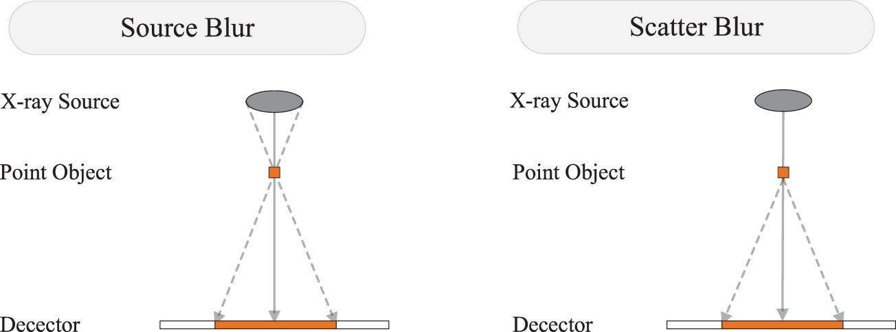
Figure 3: Schematic diagram of the principle of source blur and scattering blur. The solid gray line represents the assumed X-ray, and the gray dashed line represents the offset X-ray

We propose a Ray Correction Network (RCN) that uses an MLP to fit these offset rays from blurry images. For source blur, we consider the predicted ray offsets at the detector and the ray source in a 2D plane. Unlike natural scenes, CT scenes need to consider the scattering of rays, so the RCN also needs to predict an offset from where the ray starts. Let pidx represent the pixel index value and γ(⋅) represent the frequency encoder [20], then RCN can be expressed as:

{Δdqp,Δoqp,Δtqp}=RCN(γ(pidx)).(5)

pidx is the necessary information for RCN. We map pidx to high-frequency space, hoping that RCN can generate different correction rays according to different pixels (spatially-variant blur).

The output of the RCN constitutes the corrected rays, where Δdqp and Δoqp represents the offset of the ray on the detector and the ray source, respectively, Δtqp represents the offset of the starting position of the ray. The generated corrected ray can be expressed as:

rqp(t)=(op+Δoqp)+(t+Δtqp)⋅(dp+Δdqp).(6)

It can be observed that rqp(t) can represent any offset ray. Therefore, this blur modeling approach is not limited to source blur and scattering blur in theory. Therefore, this blur modeling method can theoretically represent any blur caused by ray offset (system vibration, coordinate offset, etc.) and is not limited to source and scattering blur.

3.4 Weight Proposal Network (WPN)

The weight of correction rays is crucial to constructing the sparse blur kernel, and the blur is strongly related to the reconstructed spatial information [41,42]. Therefore, we designed WPN to obtain the weight (wqp) of each corrected ray by fusing the depth features of the ray and the pixel position encoding. Let γ(pidx)=Eqp∈Rl×M represents the pixel position encoding, l represents encoding length, WPN can be expressed as follows:

wqp=WPN(Eqp,Sqp),(7)

where Sqp∈RC×N×M is the feature of N sampling points on the ray extracted from the penultimate layer in the reconstruction network, and C is the feature depth, which contains rich implicit spatial information.

We put the obtained weights wqp(t) and corrected rays rqp(t) into Eq. (2) to calculate the predicted blurred projection image:

I~(p)=∑iMwip⋅∑jNFΦ(rip(tj))δj.(8)

The detailed architecture of the WPN is shown in Fig. 4. Inspired by CurveNet [43], first, we impose Attentive Pooling operator [44] on Sqp in different axis, that is, scaling in a self-attention style in the axis, and summing along the axis to obtain the inter-correction rays feature vector frayp∈RC×N and inter-sampling points feature vector fsamplep∈RC×M. Then use Eqp after adjusting the feature dimension by MLP to perform matrix multiplication and Softmax operations with frayp and fsamplep respectively to calculate the mapping scores of rays and sampling points. Subsequently, frayp and fsamplep are transformed by the two MLP branches and then matrix multiplied with the mapping score, similar to the attention operation, to obtain the fine-grained feature of inter-correction rays (f^rayp) and inter-sampling points ((f^samplep). Next, these two fine-grained features are concatenated and input into MLP to obtain the final mixed feature fmixp∈RC×M. Finally, after performing the global average pooling function (GAP(⋅)) and Softmax operation (σ(⋅)) on the feature fmixp, the corrected ray weight can be obtained. The formula is as follows:

wqp=σ(GAP(fmixp)),∑i=0Mwip=1.(9)

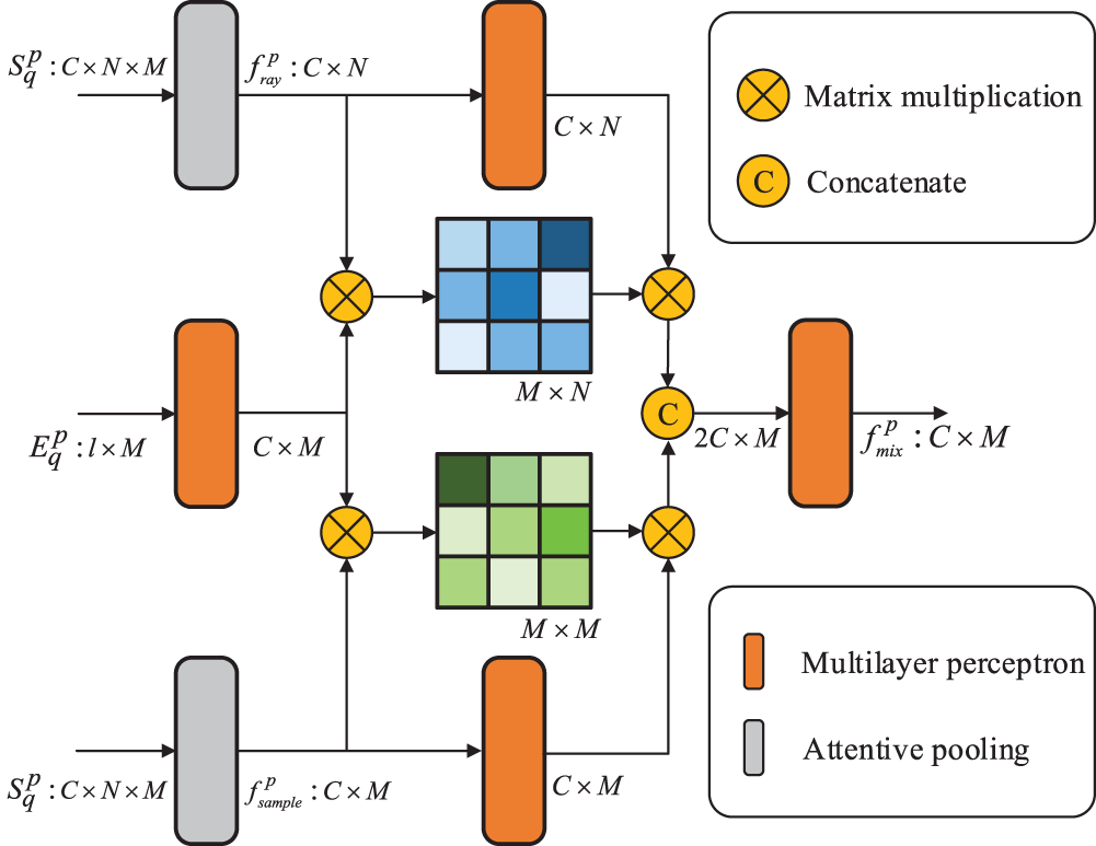
Figure 4: Weight Proposal Network (WPN) architecture

3.5 Loss Functions

The loss function includes reconstruction loss and constraint loss. The reconstruction loss is the mean square error between the predicted projection value and the measured projection value. The constraint loss is used to prevent unreasonable deviation of the corrected ray.

ℒtotal=∑p∈ℬ‖I(p)−I~(p)‖22+λcℒconstraint,(10)

where I(p) and I~(p) represent measured projection value and predicted projection value, respectively. ℬ represents the set of pixels in the batch.

Since the corrected rays have a high degree of freedom, it is easy to distort the corrected rays and the CT scene simultaneously. Therefore, we design the constraint loss to constrain the corrected rays:

ℒconstraint=|Δtv;0p|+|Δdv;0p|+λo|Δov;0p|,(11)

where subscript 0 is a fixed element of q. We constrain one of the corrected rays to be near the assumed ray. λo and λc are loss weights, which are set to 10 and 0.1, respectively, in this paper.

4  Experiments

4.1 Experimental Settings

Dataset

We perform experimental evaluations on synthetic and real datasets, respectively. The real dataset is taken by a Nikon industrial CT scanner. Since blur-free CT images (Ground truth) cannot be obtained in the real dataset, we only use the real dataset for visual qualitative evaluation. To facilitate evaluation, we selected the projection data of four objects: pepper, orange, ceramic coral, and pomegranate, which have relatively complex internal structures.

The synthetic dataset comes from the LIDC-IDRI dataset [45] and the OSV dataset [46], which contains CT data on various parts of the human body (Chest, Jaw, Foot and Abdomen). In order to simulate a real blur scene, we use a 2D anisotropic Gaussian kernel to filter the synthetic projection. The Gaussian blur function is represented as follows:

Kv(x,y)=12π(ηXv⋅ηXv)exp⁡(−12((x−ξXv)2ηXv2+(y−ξYv)2ηYv2)),(12)

where Kv represents the blur kernel of the projection with index v. ηXv and ηYv represent the variance of Gaussian function on the x and y axes, respectively, ξXv and ξYv represent the offsets of the centre coordinates of the Gaussian function, simulating coordinate offset. ηXv and ηYv are randomly selected between [6,9], and ξXv and ξYv are randomly selected between [−3, 3] for each view to simulate scenarios where the blur projection varies with different viewing angles. Besides, we add Gaussian noise with a standard deviation of 3 to each projection. This blur projection synthesis method is based on shift-invariant convolution, which ignores the shift-variance characteristics of the blur, but it is an appropriate approximation in most cases [15].

In addition, we selected 50 projections from CT images at different angles to verify the algorithm’s reconstruction quality under sparse views.

Implementation Details

The proposed method is based on PyTorch, and all experiments are done on a single RTX 4090 GPU. We use Adam optimizer with default parameters. The initial learning rate is set to 1e-3, and the learning rate is reduced to 1e-6 using the cosine decay strategy. The number of iterations for each scene is 20k, and the number of rays in each batch is 1024. The first 2k iterations only optimize the reconstruction network to initialize the scene. The CT resolution determines the sampling point of each ray. The hyperparameter settings of the multi-resolution hash encoder are kept consistent with [40]. In the reconstruction stage, we only need to query the attenuation coefficient at any position in the space to complete the reconstruction. In this paper, the quality of the reconstructed image is evaluated by peak signal-to-noise ratio (PSNR) and structural similarity (SSIM). Higher PSNR and SSIM values are preferable.

4.2 Comparisons

We compare our proposed method with five classical reconstruction methods: FDK [21], SART-TV [47], ASD-POCS [48], NAF [7] and SAX-NeRF [8]. Among them, FDK is the most commonly used analytical reconstruction method in commercial reconstruction software. SART-TV and ASD-POCS are of classical iterative reconstruction methods. NAF and SAX-NeRF are SOTA self-supervised reconstruction algorithms also based on implicit neural representations. At the same time, we introduce the current state-of-the-art X-ray image deblurring algorithm (LR [49] and RLSD [11]). For fairness, the reconstruction and deblurring algorithms we selected are not data-driven.

Due to the challenges of high radiation dose and limited scanning angle in practical applications of CT, we conducted experiments with sparse views and limited viewing angles. Table 1 shows the quantitative experimental results of all methods on synthetic datasets. It can be seen that the method proposed in this paper achieves the best results on all datasets. The average SSIM of each dataset in full view and limited angle is improved by 4.29% and 2.61%, respectively, compared with the second-best method. In addition, it can be seen that the single X-ray image deblurring technology helps improve the reconstruction quality. However, obtaining completely accurate blur kernel parameters in real scenes is tricky.

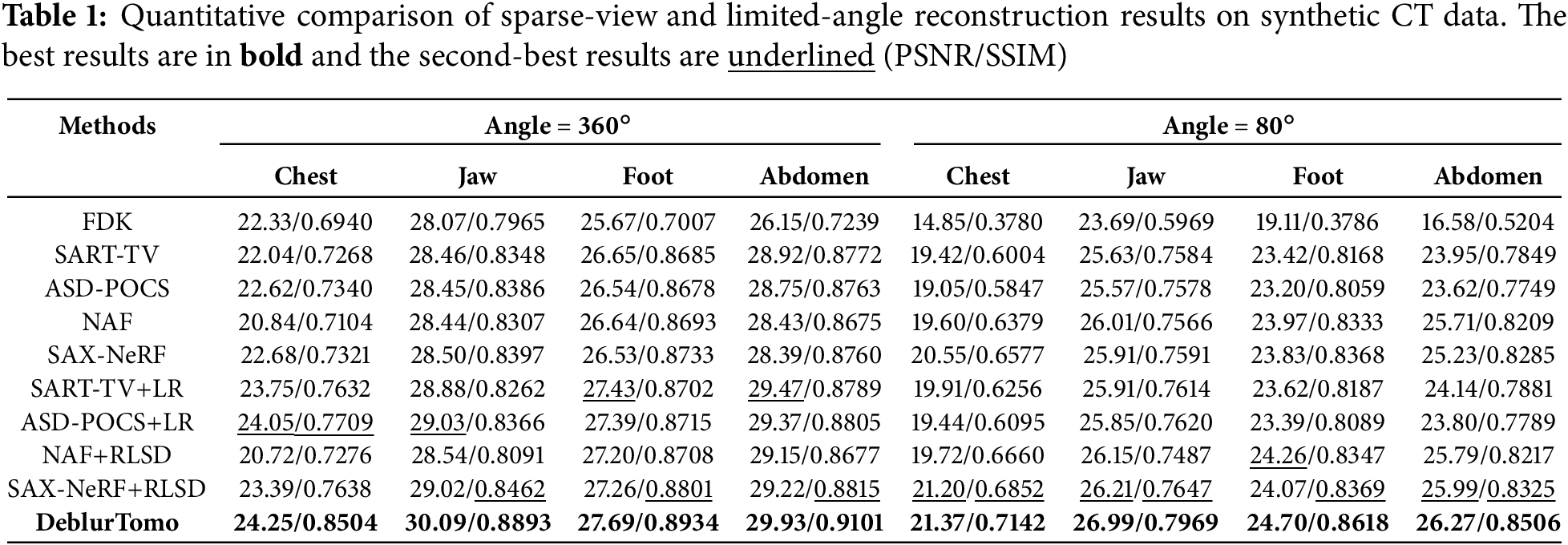
Fig. 5 presents the visualization results of each method on the synthetic dataset. It can be seen that the result of FDK has obvious artifacts with a small number of viewing angles. Single X-ray image deblurring technology does not consider the correlation between multi-view projections. In addition, although single X-ray image deblurring technology can visually make the projected image clearer, it also increases noise and ringing artifacts [11], and has limited improvement in the quality of the reconstructed image. Our method is much more satisfactory at optimizing noise and artifacts than other methods, whether in full or limited viewing angles and does not require prior information about blur kernels.

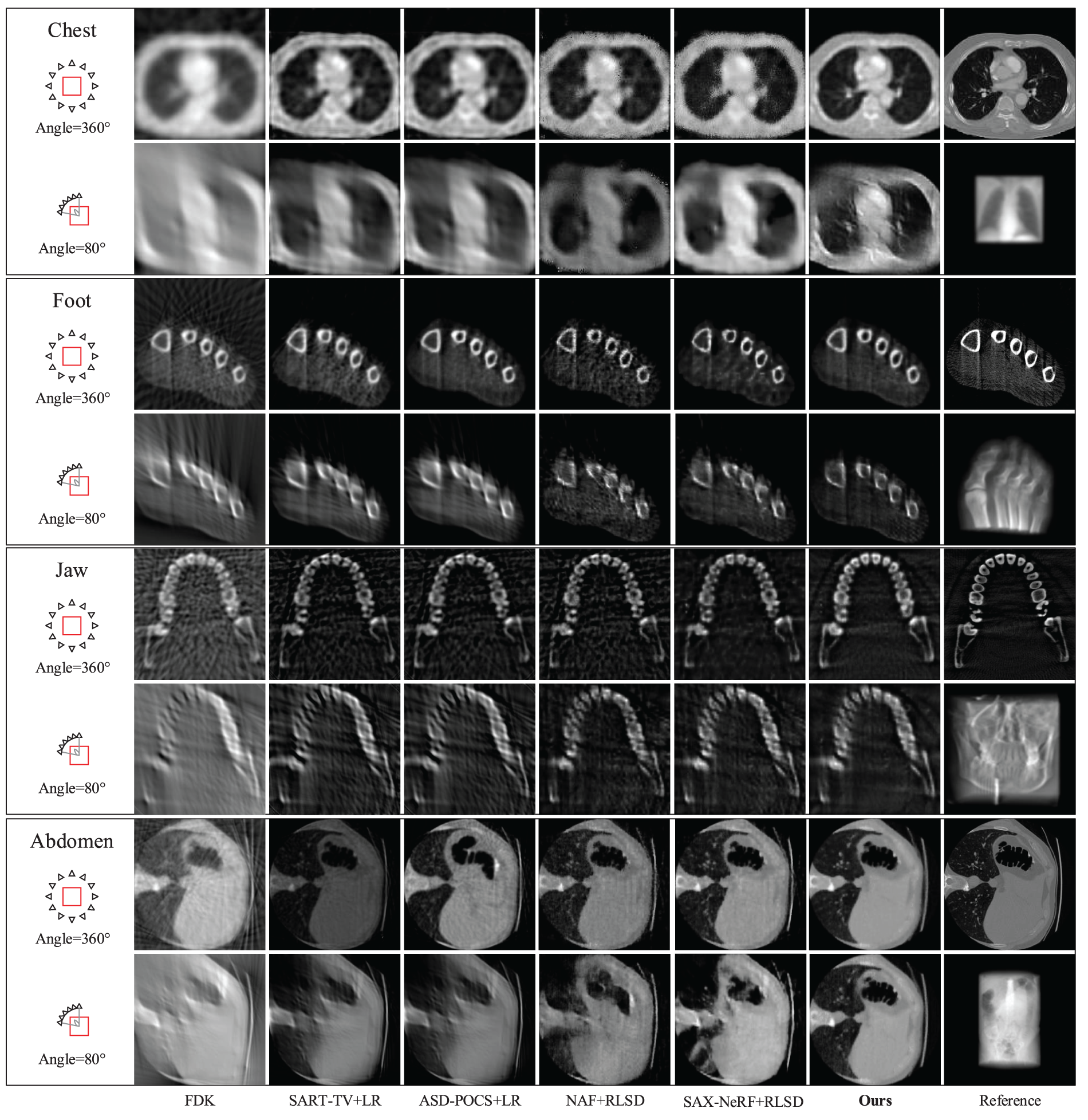
Figure 5: Qualitative comparison of sparse-view and limited-angle reconstruction results on synthetic CT data

In real datasets, single X-ray image deblurring algorithms cannot be used due to missing blur prior information. As seen from Fig. 6, SAX-NeRF uses the transformer to model ray correlation to guide the network in learning intricate spatial information. Still, the presence of blurry input introduces biases in the learned information. In addition, the Masked Local Global strategy of SAX-NeRF is not compatible with the projection size of the real dataset, which affects its performance to a certain extent. SART-TV uses TV regularization to eliminate the influence of noise on the reconstruction quality to a certain extent, but it isn’t easy to deal with artifacts caused by blurring. Our method achieves the highest visual clarity and the lowest noise and artifacts. The RCN and WPN of the proposed method utilize blur physical prior knowledge to correct for spatial bias, enabling the reconstruction network to recover the most detailed information in blurred scenes. The proposed method outperforms other methods regarding noise and artifact removal.

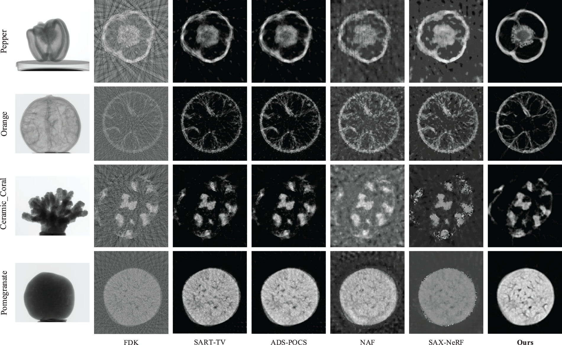
Figure 6: Qualitative comparison of each method on real CT data

4.3 Ablation Study

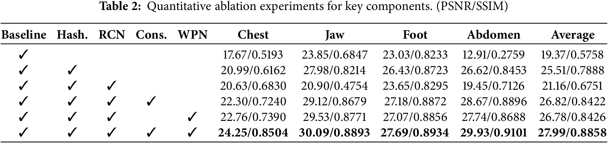
We conducted ablation experiments on DeblurTomo on a synthetic dataset to study the impact of its critical components on reconstruction quality, and the experimental results are shown in Table 2.

Hash Encoder

Compared with frequency encoder [20] (Baseline), the Hash encoder pays more attention to reconstructing the internal structure of space. Frequency encoder maps spatial coordinates to a high-dimensional space, driving the network to learn high-frequency changing spatial information. However, in CT images, the spatial information transformation is smoother. Many methods use regularization to smooth the space to remove noise. So, high-frequency features are redundant for the reconstruction network and can easily lead to overfitting. As shown in Table 2, after using the Hash encoder, SSIM is improved by 21.3%.

RCN and WPN

RCN and WPN are key parts of the ray correction. As can be seen from Fig. 7, after using RCN and WPN, the artifacts and noise of the reconstructed image are significantly reduced. In fact, RCN can also generate weights, that is, adding a weight generation branch to RCN. In order to test the effectiveness of WPN, we compared the results of the weights predicted by RCN and the weights predicted by WPN. When RCN is not used simultaneously with WPN in Table 2, RCN adds a weight branch for weight prediction. It can be seen that after using WPN, SSIM improves by an average of 4.36% on all datasets.

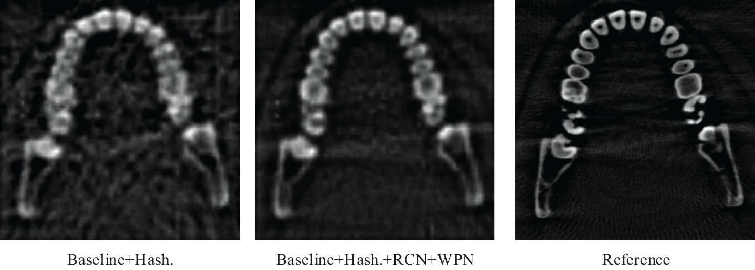
Figure 7: Reconstruction results of Jaw dataset with and without RCN and WPN. Artifacts and noise are reduced by RCN and WPN

Fig. 8 shows the reconstruction results without both WPN and constraint loss, with WPN and without constraint loss, and with both WPN and constraint loss. As seen from the left two columns of subfigures in Fig. 9, when the constraint loss on the correction rays is absent, WPN combined with spatial geometric information can prevent the corrected rays from diverting to a certain extent and reduce the reconstruction error. Therefore, WPN fusion spatial information is essential to improve the reconstruction quality.

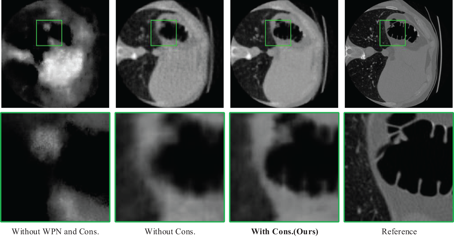
Figure 8: Reconstruction results on Abodomen dataset without using both WPN and Constraint loss, with WPN and without Constraint loss, and with both WPN and Constraint loss

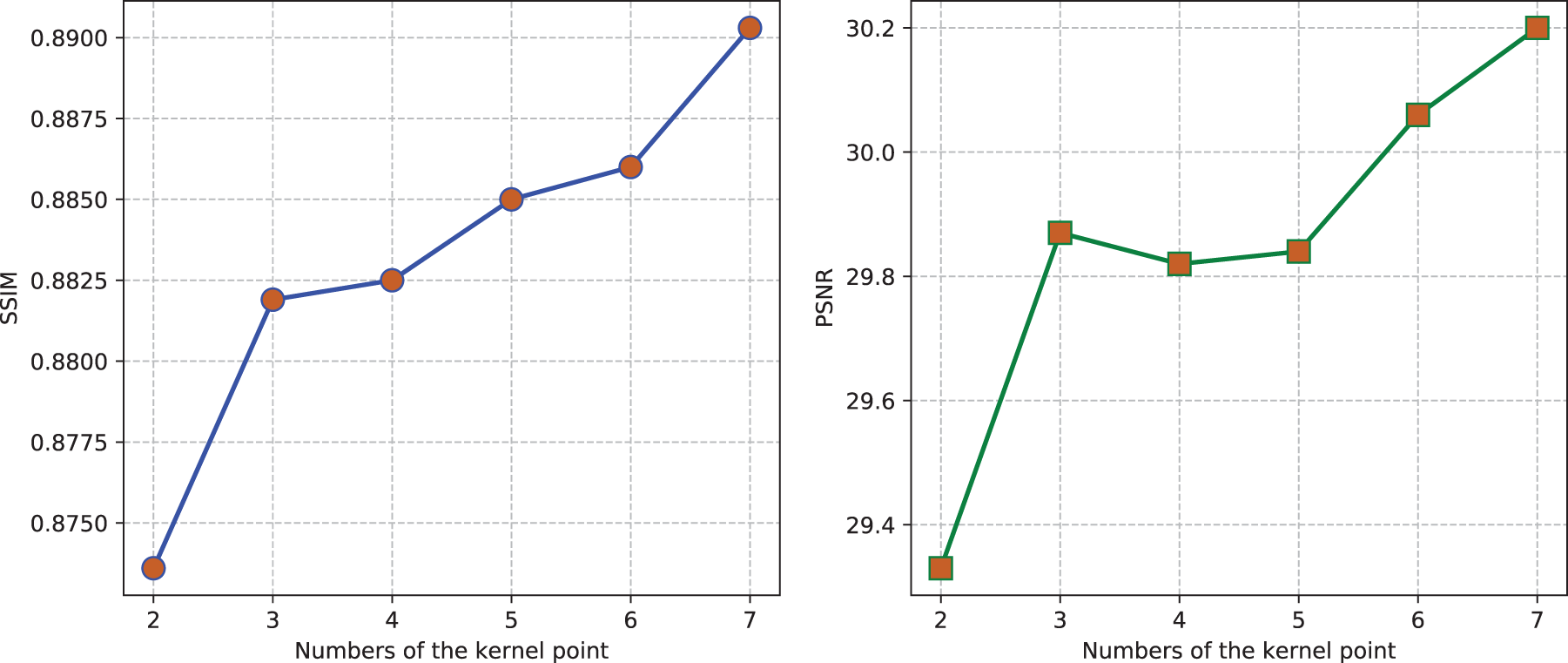
Figure 9: Comparison of reconstruction quality between different numbers of kernel points

Furthermore, we tested the effect of different numbers of kernel points on the reconstruction quality. Fig. 9 shows that as the number of kernel points increases, the reconstruction quality rises steadily. Increasing the number of kernel points enables the network to better approximate the blur process, albeit at the cost of higher computational resources. Considering this trade-off, we set the number of kernel points to 5 (M=5).

Constraint Loss

As mentioned in Section 3.5, the constraint loss can prevent the predicted corrected ray and CT scene from being distorted simultaneously. As can be seen from Fig. 8, not adding constraint loss can easily cause the reconstructed image to be blurred in detail, although the blur is improved after adding WPN. In general, using Constraint loss can effectively improve the reconstruction quality.

5  Discussion

Previous experimental results show demonstrate that DeblurTomo significantly outperforms baseline methods across both real and synthetic CT datasets. In addition, DeblurTomo also demonstrates several other advantages. First, unlike most learning-based methods that require clean real data or pre-trained networks, DeblurTomo relies entirely on the blurred projection itself, which makes it more applicable to real-world clinical or industrial environments. Second, by embedding blur correction directly into the reconstruction process through RCN and WPN, DeblurTomo avoids the two-step deblurring and then reconstruction method, which usually amplifies noise or introduces inconsistencies between views. Third, the design of DeblurTomo is not limited to a specific kernel type or known blur model. Its learnable formula enables it to adapt to various unknown or shifted blur conditions, making it widely applicable.

However, the method also has some limitations. While the correction mechanism is highly flexible, it can lead to coupled deformation of both the reconstructed scene and the corrected rays, especially when the constraint loss is insufficient to regularize the solution. Moreover, increasing the number of kernel points improves blur modeling accuracy, but at the cost of significantly higher computational complexity and memory consumption.

For future work, we plan to incorporate Gaussian splatting techniques to reduce the need for frequent sampling-point queries and improve reconstruction speed. We also aim to integrate more physical priors, such as ray source size, source-to-detector distance, and object geometry, to constrain the correction process further and improve blur modeling accuracy.

6  Conclusion

This paper proposes the first self-supervised implicit neural representation CT deblurring reconstruction algorithm. We model the blur as multiple offset rays according to the physical process of blur and fit these rays through multi-view consistency and geometric information. This method helps to calibrate the 3D scene and reduce artifacts in the reconstructed image. Experiments on multiple real and synthetic CT datasets show that DeblurTomo outperforms other existing methods in blurry scenes. Although our method is currently used on CT images, we believe similar blur modeling methods can be applied to other medical imaging scenarios such as Magnetic Resonance Imaging and Positron Emission Tomography.

Acknowledgement: Not applicable.

Funding Statement: This work was supported in part by the National Natural Science Foundation of China under Grants 62472434 and 62402171; in part by the National Key Research and Development Program of China under Grant 2022YFF1203001; in part by the Science and Technology Innovation Program of Hunan Province under Grant 2022RC3061; and in part by the Sci-Tech Innovation 2030 Agenda under Grant 2023ZD0508600.

Author Contributions: The authors confirm contribution to the paper as follows: study conception and design, Qingyang Zhou and Guofeng Lu; writing—original draft preparation, Qingyang Zhou and Yunfan Ye, writing—review and editing, Yunfan Ye and Zhiping Cai; data curation, Guofeng Lu; supervision, Yunfan Ye; funding acquisition, Zhiping Cai. All authors reviewed the results and approved the final version of the manuscript.

Availability of Data and Materials: The datasets employed in this study (LIDC-IDRI and OSV) are publicly available benchmark datasets. Interested researchers can obtain the data from their respective official repositories under the terms specified by the dataset publishers.

Ethics Approval: Not applicable.

Conflicts of Interest: The authors declare no conflicts of interest to report regarding the present study.

References

1. Kiljunen T, Kaasalainen T, Suomalainen A, Kortesniemi M. Dental cone beam CT: a review. Physica Medica. 2015;31(8):844–60. doi:10.1016/j.ejmp.2015.09.004. [Google Scholar] [PubMed] [CrossRef]

2. Zhou Q, Qin J, Xiang X, Tan Y, Ren Y. MOLS-Net: multi-organ and lesion segmentation network based on sequence feature pyramid and attention mechanism for aortic dissection diagnosis. Knowl Based Syst. 2022;239(17):107853. doi:10.1016/j.knosys.2021.107853. [Google Scholar] [CrossRef]

3. Vásárhelyi L, Kónya Z, Kukovecz Á, Vajtai R. Microcomputed tomography-based characterization of advanced materials: a review. Mater Today Adv. 2020;8(2018):100084. doi:10.1016/j.mtadv.2020.100084. [Google Scholar] [CrossRef]

4. Mohan K, Panas R, Cuadra J. A systems approach to prediction and mitigation of radiographic blur. In: Summer Topical Meeting on Advancing Precision in Additive Manufacturing; 2018; Berkeley, CA, USA. p. 211–6. [Google Scholar]

5. Li H, Kingston A, Myers G, Recur B, Sheppard A. 3D X-ray source deblurring in high cone-angle micro-CT. IEEE Trans Nucl Sci. 2015;62(5):2075–84. doi:10.1109/TNS.2015.2435782. [Google Scholar] [CrossRef]

6. Wang Q, Zhu Y, Li H. Imaging model for the scintillator and its application to digital radiography image enhancement. Opt Express. 2015;23(26):33753–76. doi:10.1364/OE.23.033753. [Google Scholar] [PubMed] [CrossRef]

7. Zha R, Zhang Y, Li H. NAF: neural attenuation fields for sparse-view CBCT reconstruction. In: International Conference on Medical Image Computing and Computer-Assisted Intervention. Cham: Springer Nature Switzerland; 2022. p. 442–52. doi:10.1007/978-3-031-16446-0_42. [Google Scholar] [CrossRef]

8. Cai Y, Wang J, Yuille A, Zhou Z, Wang A. Structure-aware sparse-view X-ray 3D reconstruction. In: Proceedings of the IEEE/CVF Conference on Computer Vision and Pattern Recognition; 2024; Seattle, WA, USA. p. 11174–83. [Google Scholar]

9. von Wittenau AS, Logan C, Aufderheide Iii M, Slone D. Blurring artifacts in megavoltage radiography with a flat-panel imaging system: comparison of Monte Carlo simulations with measurements. Med Phy. 2002;29(11):2559–70. doi:10.1118/1.1513159. [Google Scholar] [PubMed] [CrossRef]

10. Joshi N, Szeliski R, Kriegman DJ. PSF estimation using sharp edge prediction. In: 2008 IEEE Conference on Computer Vision and Pattern Recognition. Anchorage, AK, USA: IEEE; 2008. p. 1–8. doi:10.1109/CVPR.2008.4587834. [Google Scholar] [CrossRef]

11. Mohan KA, Panas RM, Cuadra JA. SABER: a systems approach to blur estimation and reduction in X-ray imaging. IEEE Trans Image Process. 2020;29:7751–64. doi:10.1109/TIP.2020.3006339. [Google Scholar] [CrossRef]

12. Puetter R, Gosnell T, Yahil A. Digital image reconstruction: deblurring and denoising. Annu Rev Astron Astrophys. 2005;43(1):139–94. doi:10.1146/annurev.astro.43.112904.104850. [Google Scholar] [CrossRef]

13. Hussien MN, Saripan MI. Computed tomography soft tissue restoration using Wiener filter. In: 2010 IEEE Student Conference on Research and Development (SCOReD). Kuala Lumpur, Malaysia: IEEE; 2010. p. 415–20. doi:10.1109/SCORED.2010.5704045. [Google Scholar] [CrossRef]

14. Tilley S, Siewerdsen JH, Stayman JW. Model-based iterative reconstruction for flat-panel cone-beam CT with focal spot blur, detector blur, and correlated noise. Phys Med Biol. 2015;61(1):296–319. doi:10.1088/0031-9155/61/1/296. [Google Scholar] [PubMed] [CrossRef]

15. Tilley S, Jacobson M, Cao Q, Brehler M, Sisniega A, Zbijewski W, et al. Penalized-likelihood reconstruction with high-fidelity measurement models for high-resolution cone-beam imaging. IEEE Trans Med Imag. 2017;37(4):988–99. doi:10.1109/TMI.2017.2779406. [Google Scholar] [PubMed] [CrossRef]

16. Tilley S, Zbijewski W, Stayman JW. High-fidelity modeling of shift-variant focal-spot blur for high-resolution CT. In: The 14th International Meeting on Fully Three-Dimensional Image Reconstruction in Radiology and Nuclear Medicine; 2017. p.752–9. doi:10.12059/Fully3D.2017-11-3201031. [Google Scholar] [CrossRef]

17. Xiao Y, Peng W, Wang Y. In-situ NDT CT image restoration method for concrete based on deep learning by modeling non-ideal focal spot. NDT E Int. 2024;142(12):103018. doi:10.1016/j.ndteint.2023.103018. [Google Scholar] [CrossRef]

18. Nuyts J, De Man B, Fessler JA, Zbijewski W, Beekman FJ. Modelling the physics in the iterative reconstruction for transmission computed tomography. Phys Med Biol. 2013;58(12):R63–96. doi:10.1088/0031-9155/58/12/R63. [Google Scholar] [PubMed] [CrossRef]

19. Alenezi F, Santosh K. Geometric regularized hopfield neural network for medical image enhancement. Int J Biomed Imag. 2021;2021(1):6664569. doi:10.1155/2021/6664569. [Google Scholar] [PubMed] [CrossRef]

20. Mildenhall B, Srinivasan PP, Tancik M, Barron JT, Ramamoorthi R, Nerf Ng R. Representing scenes as neural radiance fields for view synthesis. Commun ACM. 2021;65(1):99–106. doi:10.1145/3503250. [Google Scholar] [CrossRef]

21. Feldkamp LA, Davis LC, Kress JW. Practical cone-beam algorithm. J Opti Soc Am A. 1984;1(6):612–9. doi:10.1364/JOSAA.1.000612. [Google Scholar] [CrossRef]

22. Andersen AH, Kak AC. Simultaneous algebraic reconstruction technique (SARTa superior implementation of the ART algorithm. Ultrasonic Imag. 1984;6(1):81–94. doi:10.1177/016173468400600107. [Google Scholar] [PubMed] [CrossRef]

23. Gao Y, Bian Z, Huang J, Zhang Y, Niu S, Feng Q, et al. Low-dose X-ray computed tomography image reconstruction with a combined low-mAs and sparse-view protocol. Opti Express. 2014;22(12):15190–210. doi:10.1364/OE.22.015190. [Google Scholar] [PubMed] [CrossRef]

24. Niu S, Gao Y, Bian Z, Huang J, Chen W, Yu G, et al. Sparse-view X-ray CT reconstruction via total generalized variation regularization. Phys Medi Biol. 2014;59(12):2997–3017. doi:10.1088/0031-9155/59/12/2997. [Google Scholar] [PubMed] [CrossRef]

25. Huang Y, Taubmann O, Huang X, Haase V, Lauritsch G, Maier A. Scale-space anisotropic total variation for limited angle tomography. IEEE Trans Radiat Plasma Med Sci. 2018;2(4):307–14. doi:10.1109/TRPMS.2018.2824400. [Google Scholar] [CrossRef]

26. Xu M, Hu D, Luo F, Liu F, Wang S, Wu W. Limited-angle X-ray CT reconstruction using image gradient l0-norm with dictionary learning. IEEE Trans Radiat Plasma Med Sci. 2020;5(1):78–87. doi:10.1109/TRPMS.2020.2991887. [Google Scholar] [CrossRef]

27. Anastasovitis E, Roumeliotis M. Enhanced and combined representations in extended reality through creative industries. Appl Syst Innov. 2024;7(4):55. doi:10.3390/asi7040055. [Google Scholar] [CrossRef]

28. Anastasovitis E, Roumeliotis M. Transforming computed tomography scans into a full-immersive virtual museum for the Antikythera Mechanism. Digit Appl Archaeol Cult Herit. 2023;28(1):e00259. doi:10.1016/j.daach.2023.e00259. [Google Scholar] [CrossRef]

29. Fish D, Brinicombe A, Pike E, Walker J. Blind deconvolution by means of the Richardson-Lucy algorithm. J Opti Soc Am A. 1995;12(1):58–65. doi:10.1364/JOSAA.12.000058. [Google Scholar] [CrossRef]

30. You C, Li G, Zhang Y, Zhang X, Shan H, Li M, et al. CT super-resolution GAN constrained by the identical, residual, and cycle learning ensemble (GAN-CIRCLE). IEEE Trans Med Imag. 2019;39(1):188–203. doi:10.1109/TMI.2019.2922960. [Google Scholar] [PubMed] [CrossRef]

31. Kim H, Lee H, Lee D. Deep learning-based computed tomographic image super-resolution via wavelet embedding. Radiat Phys Chem. 2023;205(2):110718. doi:10.1016/j.radphyschem.2022.110718. [Google Scholar] [PubMed] [CrossRef]

32. Li Y, Iwamoto Y, Lin L, Xu R, Tong R, Chen YW. VolumeNet: a lightweight parallel network for super-resolution of MR and CT volumetric data. IEEE Trans Image Process. 2021;30:4840–54. doi:10.1109/TIP.2021.3076285. [Google Scholar] [PubMed] [CrossRef]

33. Lei Y, Niu C, Zhang J, Wang G, Shan H. CT image denoising and deblurring with deep learning: current status and perspectives. IEEE Trans Radiat Plasma Med Sci. 2023;8(2):153–72. doi:10.1109/TRPMS.2023.3341903. [Google Scholar] [CrossRef]

34. Ma L, Li X, Liao J, Zhang Q, Wang X, Wang J, et al. Deblur-NERF: neural radiance fields from blurry images. In: Proceedings of the IEEE/CVF Conference on Computer Vision and Pattern Recognition; 2022; New Orleans, LA, USA. p. 12861–70. doi:10.1109/CVPR52688.2022.01252. [Google Scholar] [CrossRef]

35. Lee D, Lee M, Shin C, Lee S. Deblurred neural radiance field with physical scene priors. In: Proceedings of the IEEE/CVF Conference on Computer Vision and Pattern Recognition; 2023; Vancouver, BC, Canada. p. 12386–96. doi:10.1109/CVPR52729.2023.01192. [Google Scholar] [CrossRef]

36. Liu YL, Gao C, Meuleman A, Tseng HY, Saraf A, Kim C, et al. Robust dynamic radiance fields. In: Proceedings of the IEEE/CVF Conference on Computer Vision and Pattern Recognition; 2023; Vancouver, BC, Canada. p. 13–23. [Google Scholar]

37. Molaei A, Aminimehr A, Tavakoli A, Kazerouni A, Azad B, Azad R, et al. Implicit neural representation in medical imaging: a comparative survey. In: Proceedings of the IEEE/CVF International Conference on Computer Vision Workshops; 2023; Paris, France. p. 2381–91. doi:10.1109/ICCVW60793.2023.00252. [Google Scholar] [CrossRef]

38. Rückert D, Wang Y, Li R, Idoughi R, Heidrich W. Neural adaptive tomography. ACM Trans Grap (TOG). 2022;41(4):1–13. doi:10.1145/3528223.3530121. [Google Scholar] [CrossRef]

39. Kak AC, Slaney M. Principles of computerized tomographic imaging. Philadelphia, PA, USA: SIAM; 2001. [Google Scholar]

40. Müller T, Evans A, Schied C, Keller A. Instant neural graphics primitives with a multiresolution hash encoding. ACM Trans Grap. 2022;41(4):1–15. doi:10.1145/3528223.3530127. [Google Scholar] [CrossRef]

41. Tilley S, Zbijewski W, Siewerdsen JH, Stayman JW. Modeling shift-variant X-ray focal spot blur for high-resolution flat-panel cone-beam CT. In: Conference Proceedings. International Conference on Image Formation in X-Ray Computed Tomography. Bellingham, WA, USA: NIH Public Access; 2016. Vol. 2016, p. 463–6. [Google Scholar]

42. Hehn L, Tilley S, Pfeiffer F, Stayman JW. Blind deconvolution in model-based iterative reconstruction for CT using a normalized sparsity measure. Phys Med Biol. 2019;64(21):215010. doi:10.1088/1361-6560/ab489e. [Google Scholar] [PubMed] [CrossRef]

43. Xiang T, Zhang C, Song Y, Yu J, Cai W. Walk in the cloud: learning curves for point clouds shape analysis. In: Proceedings of the IEEE/CVF International Conference on Computer Vision; 2021; Montreal, QC, Canada. p. 915–24. doi:10.1109/ICCV48922.2021.00095. [Google Scholar] [CrossRef]

44. Hu Q, Yang B, Xie L, Rosa S, Guo Y, Wang Z, et al. Randla-net: efficient semantic segmentation of large-scale point clouds. In: Proceedings of the IEEE/CVF Conference on Computer Vision and Pattern Recognition; 2020; Seattle, WA, USA. p. 11108–17. doi:10.1109/CVPR42600.2020.01112. [Google Scholar] [CrossRef]

45. Armato IIISG, McLennan G, Bidaut L, McNitt-Gray MF, Meyer CR, Reeves AP, et al. The lung image database consortium (LIDC) and image database resource initiative (IDRIa completed reference database of lung nodules on CT scans. Med Phys. 2011;38(2):915–31. doi:10.1118/1.3528204. [Google Scholar] [CrossRef]

46. Klacansky P. Open scientific visualization datasets; 2022. [Online]. [cited 2025 May 22]. Available from: https://klacansky.com/open-scivis-datasets/. [Google Scholar]

47. Zang G, Aly M, Idoughi R, Wonka P, Heidrich W. Super-resolution and sparse view CT reconstruction. In: Proceedings of the European Conference on Computer Vision (ECCV); 2018; Munich, Germany. p. 137–53. [Google Scholar]

48. Sidky EY, Pan X. Image reconstruction in circular cone-beam computed tomography by constrained, total-variation minimization. Phys Med Biol. 2008;53(17):4777. doi:10.1088/0031-9155/53/17/021. [Google Scholar] [PubMed] [CrossRef]

49. Richardson WH. Bayesian-based iterative method of image restoration. J Opti Soc Am. 1972;62(1):55–9. doi:10.1364/JOSA.62.000055. [Google Scholar] [CrossRef]