HybridLSTM: An Innovative Method for Road Scene Categorization Employing Hybrid Features

1  Introduction

The rapid advancement of autonomous vehicles and intelligent transportation systems has underscored the critical importance of accurate road scene classification. This capability enables vehicles to interpret their surroundings effectively, ensuring safer navigation and improved decision-making. Road scenes encompass a diverse array of visual elements—including objects, textures, and environmental features—that must be identified and analyzed in real time. Traditional methods that rely on single-feature analysis often fall short in addressing the complexity and variability inherent in these scenarios. Consequently, there is a pressing need for robust approaches capable of efficiently handling both global and localized details.

Recent advancements in deep learning and computer vision have facilitated the development of hybrid techniques that integrate multiple feature types for enhanced scene understanding. By combining object-based features, scene-level global representations, and handcrafted low-level descriptors, these approaches provide a comprehensive analysis of road scenes. In this context, this study introduces HybridLSTM, an innovative framework for road scene classification that leverages the strengths of Long Short-Term Memory (LSTM) networks. HybridLSTM effectively incorporates hybrid features derived from state-of-the-art models, including YOLOv5 for object detection, VGG19 for both object-level and scene-level information, as well as various handcrafted descriptors for fine-grained analysis.

The proposed framework is rigorously evaluated on diverse datasets such as Places-365, BDD100K, LabelMe, and KITTI, demonstrating remarkable cross-domain performance. It achieves a classification accuracy of 96.3%, precision of 95.8%, recall of 96.1%, and an F1-score of 96.0% across categories like crosswalks, highways, overpass tunnels, and parking areas, outperforming previous approaches. These results underscore the potential of hybrid feature integration to advance road scene classification, effectively addressing the critical challenges faced by contemporary autonomous systems. The insights gained from this research are invaluable in the pursuit of developing safer and more efficient autonomous vehicle technologies.

1.1 The Motivation for Research

The developing reliance on self-sufficient automobiles and sensible transportation structures needs accurate street scene class. Despite advancements in laptop imaginative and prescient and deep learning, challenges persist in achieving reliable classification across diverse and complicated street environments. This work proposes a hybrid approach combining item detection, deep gaining knowledge of, and handcrafted functions. The framework aims to offer a comprehensive understanding of street scenes, making sure its applicability in real-global self-sufficient structures and enhancing safety and performance in transportation.

1.2 The Risk Aspect

The proposed road scene class framework, at the same time as innovative and strong, consists of sure chance elements that want to be addressed:

•   One big risk is the high computational complexity related to the hybrid feature fusion and LSTM-based temporal modeling, which may lead to long latencies that can hinder real-time performance on resource-constrained edge devices.

•   One primary chance is the high computational complexity involved in integrating the LSTM community with many characteristic extraction techniques (handmade, scene-level, and item-level), which may impair actual-time overall performance in packages involving independent cars.

•   Furthermore, because the model relies upon on wonderful datasets like BDD100K, KITTI, and others, its performance can also go through in conditions with unknown or low-best records, such dim illumination, converting weather, or occlusions.

•   The sensitivity of the system to inaccurate or partial object detection by YOLOv5 poses an additional danger as it may cause mistakes to spread throughout the classification pipeline.

•   Finally, the absence of uniform performance standards for various datasets might make it difficult to evaluate the system’s resilience and generalizability under a variety of road conditions. Deploying this technology in actual autonomous systems will require addressing these issues.

1.3 Major Contributions

The work claims the following contributions:

❖   Propose a novel framework for road scene classification by integrating hybrid features with a Long Short-Term Memory (LSTM) network.

❖   Utilize YOLOv5 for accurate object detection, followed by VGG19 for extracting detailed object-level features from the detected objects.

❖   Employ a modified VGG19 network for capturing global scene-level features, ensuring comprehensive representation of the road scene.

❖   Incorporate handcrafted descriptors to extract fine-grained details, providing complementary information to deep learning-based features.

❖   Demonstrate the effectiveness of the proposed hybrid approach in classifying road scenes into four distinct categories: crosswalk, highway, over tunnel, and parking.

The article has been conducted as follows: Review of Section 2 is related to recent state-of-the-art classification. Section 3 has a detail of material and methods including information about the dataset and proposed Visual Classification System (VCS). Section 4 presents the results and discussion, focusing on the analysis of the system suggested in four categories of road visual classification. Section 5 discusses the system performance on the real-time road scene frame captured in Nagpur, India. Finally, Section 6 concludes the article.

2  Survey of Relevant Research

Road Visual Classification has drawn significant attention in recent years, proposing to solve the challenges generated by complex and diverse visual environments with different methods. The initial approach was mainly based on the handicapped characteristics, such as descriptive of the composition, colour, and edge, who, despite their simplicity, often struggled with generalization in different datasets. With the advent of Deep Learning, the types of global visual features have been widely adopted for VGG, ResNET and their Quasi-Recurrent Neural Networks (QRNN). In addition, Object Budget Detection models such as yolo and fast R-CNN are beneficial to identify the main objects in the scenes, helping to help in a better relevant understanding. Hybrid methods connecting global, object budget-Levels and Crafts have enhanced complementary information. Recent studies have also found the use of a successive model, such as a long-term short-term memory (LSTM) network, which enables strong classification in complex views, to model temporary dependence and related relationships, to model temporary dependence and related relationships. Inside the scenes. However, such an outline is necessary to effectively integrate these progresses effectively to achieve high accuracy in various datasets and challenging circumstances, a difference wants to address this study.

Scenes on the road and road are rich in detail, representing the abundance of scenes for analysis. The effectiveness of the automatic Sean Classification System is important for accurate predictions of labels enhancing automobile safety. Some studies have successfully introduced a strong image classification framework that effectively distinguishes a wide range of image categories [1,2]. Deep networks constantly demonstrate exquisite operations and are constantly optimized according to the Object Budget-Centric ImageNet Classification Standards [3].

Moreover, there is significant potential for further advancements in scene categorization to improve visual perception. The research featured in [4] has already made notable strides in scene classification and recognition, employing a dataset of 2.5 million road scenes across 205 categories. Wang et al. [5] introduced a pedestrian tracking algorithm that leverage sparse models to improve tracking performance in urban road scenes. The approach demonstrates greater accuracy and stability in dynamic and densely populated traffic environments. In the field of robotics, broader studies have been conducted for scene classification like semantic mapping [6,7]. In order to improve classification performance on large-scale datasets utilizing pre-trained VGG-16 networks, the study suggests a scene picture representation technique that makes use of foreground, background, and hybrid characteristics [8], and non-mobile objects which include bridges, underpass tunnels, over bridges, constructions, etc. [9]. In most of the datasets, the scene images in general do not possess labels but mere object-level attributes provide a general picture of the class labels [10]. About videos, labels associated with complete clips are available without frame-based annotations. Analysis based on visual perception is tedious and time-consuming for automotive datasets.

In the real world, automobiles are provided with a variety of sensors, radars, and geographical positioning systems, to acquire real-time on-road traffic conditions [11,12]. Path following and driving decisions rely on the high-level semantic information of the vehicle’s current geographical coordinates. Such intelligent systems accelerate a car on an open highway, slow down approaching a school or medical centre, stop at a red signal, adopt an antiskid mechanism during rains and snowy paths, make use of fog lights during the foggy atmosphere, de-accelerate the vehicle for drivers’ drowsiness and drunk conditions, etc. [13,14]. Researchers proposed various methods to reduce traffic accidents and driver stress through better object detection and classification. Bachute and Subhedar [15] explored machine learning architectures for autonomous vehicles, while Al-refai et al. [16] applied Yolov3 to detect real-time road objects. Qaddoura and colleagues [17,18] emphasized the forecast of traffic characteristics for safer navigation. Kajiwara [19] focused on monitoring driver status using physiological data, and Shen et al. [20] introduced convolutionary chart networks for pedestrian detection. These approaches highlight the need for quick and accurate scene analysis to improve autonomous decision-making systems.

Initially, PASCAL VOC competition was regarded as the image classification benchmark dataset and the systems introduced in [21,22] based on low-level local features were regarded as the best approaches. The authors used a non-linear machine-learned classifier such as SVM. A Gaussian mixture model was fitted aggregating the local descriptor features encoded with statistics through spatial Fisher vectors and SVM [23,24]. It was in 2012, that the use of AlexNet [25] based on CNN outperformed the work on the ImageNet dataset. The image classification accuracy was improved later with the next generation deep networks such as GoogleNet [26], VGGNet [27], and ResNet [28], which considered the depth of the networks as a crucial parameter for the success of classification.

In earlier work used in traffic scene classification, objects in the scenes were of importance and object-based features, their probabilities were used to classify scenes [29]. Along with objects, scene semantics segmentation labels were also used to distinguish classes that included pedestrians, road layouts, and obstacles in front of the vehicles [30]. Traffic scenes were understood using the semantic labels in [31,32] where CNN was trained on scene images acquired at a location under different lighting conditions and weather. Zou et al. [33] proposed a deep neural network-based lane detection model that improves accuracy in crowded road situations. Its sensitivity to occluded and unstructured environments is problematic, requiring more generalized road scene classification techniques.

To address the aforementioned issue, scene images from four distinct datasets were analyzed, categorized into four classes: parking, highways, overpass tunnels, and crosswalks. To increase the complexity of the scene classification task, the tunnel and overpass categories were merged into a single class. Additionally, the road scene images taken into consideration included scenes with diverse types of weather and atmospheric conditions, including day, night, rain, snow, etc. Four distinct datasets were used to gather the images: BDD100K, LabelMe, KITTI, and Places365. Wang et al. [34] proposed a pre-visualization detection and classification structure that founds visual and laser data using deep learning for unstructured scenes. The method enhances the accuracy of perception in complex off-road environments through multimodal resource integration. Recent advances in understanding the road scene leveraged deep learning for improved classification and segmentation. Zhou et al. [35] introduced a deep learning structure that significantly improved the interpretation of the road scene through hierarchical resource extraction. Guo et al. [36] proposed a rexnet care model that addressed class imbalance questions in long-tailed road scenes data sets, reaching higher accuracy through attention mechanisms. Prykhodchenko and Skruch [37] have developed a learning approach to various tasks capable of simultaneously predicting the kind of scene, time and climate, thus expanding the contextual awareness of classification systems.

The authors in [38] classified the static road scene objects accurately using an improved deep-learning network based on the PointNet++ network. They found that the existing PointNet++ network suffered insufficient feature learning and poor accuracy. They introduced LO-Net to extract significant objects from the images acquired using the LiDAR system. They optimized the network by incorporating three different modules that included GraphConv, Unit module, and the J-PSPP. They were used to combine various feature-learning techniques in a layer-wise optimized network. They obtained better classification accuracy on three distinct datasets that included the ModelNet 40, and 10 datasets and the Sydney Urban Objects. However, their framework obtained 98.5% accuracy over the Road9 dataset images. They concluded that their proposed framework exhibits generalization capabilities and showed effectiveness and robustness. However, their framework was complex.

Gurkan Dogan and Burhan Ergen [39] worked on object segmentation from traffic scenes using CNN. They introduced a new module called the attention atrous feature pooling and placed it between the encoder and the decoder which served to acquire multiscale details and add attentional features for objects of various dimensions. They claimed that their module assisted in more effective learning over the CamVid dataset. They showed that their model obtained an average IoU concerning others approximately 2% higher. Arindam Chaudhari [40] addressed the issues regarding the accurate segmentation of vehicles from the traffic scenes. The author focused on the difficulties of high and low-density traffic, background with clutter, and occlusions. The article also considered the shadow and illumination issues. The vehicles were segmented using the Faster-RCNN deep learning network via four steps that included adaptive background minimization, subnet operation, initial refinement, and the topological active networks. The author found that the new framework using the Faster RCNN improved the segmentation accuracy.

Du et al. [41] contributed by launching the Toronto-RDMK database and proposing RDMKNET, a robust model for rating and segmentation of road marking, advancing the availability of large-scale noted data for smart transport systems. Majd Alqarqaz et al. [42] developed an intelligent object classification module for autonomous vehicles to classify 7 different objects. They focused on the early detection of the objects using machine learning and conducted research over different datasets. The scene images were taken from two datasets including the Udacity and the BDD100K. They pre-processed data by removing the missing values and duplicate entries and carried data partitioning in an 80:20 ratio for training and testing purposes. Six machine learning algorithms were applied, and the performance was measured in terms of five performance metrics including classification accuracy, precision, recall, G-mean, and the F1-score. The object classification module suggested by them obtained poor results concerning the precision whereas other parameters were good. To increase the segmentation and detection accuracy, a hybrid strategy that included characteristics from two object identification models—YOLO and Fast RCNN—was employed [43]. To enhance segmentation and classification, they made advantage of YOLO’s capabilities in conjunction with Fast RCNN’s region of interest. Additionally, they eliminated the region proposal network and trained the network on 10,000 pictures, which shortened the processing time of Fast RCNN. The accuracy they achieved was 5–7% higher than that of the YOLO network alone.

Khan and Basalamah [44] introduced a deep learning structure of various branches for classification of terrestrial scenes using satellite images. Its approach improves the accuracy of the classification, effectively capturing several space resources in various network branches. The faster RCNN network was modified to extract local semantic features by adding residual attention structure [45], while an enhanced Inception network was used to extract global features. The ELU function and Leaky ReLU are used in the latter network to learn the convolution kernel’s redundancy. To further achieve the scene categorization, both attributes were combined. The author created their dataset in order to categorize scenarios for autonomous vehicles. In this work, heterogeneous road agents are not considered. Narlawar and Pete [46] proposed a method for occluded face recognition by applying contrast correction and edge-preserving enhancement techniques, leading to the extraction of optimum features from the CelebA dataset.

Table 1 below shows the comparative analysis of techniques for road scene classification in autonomous driving.

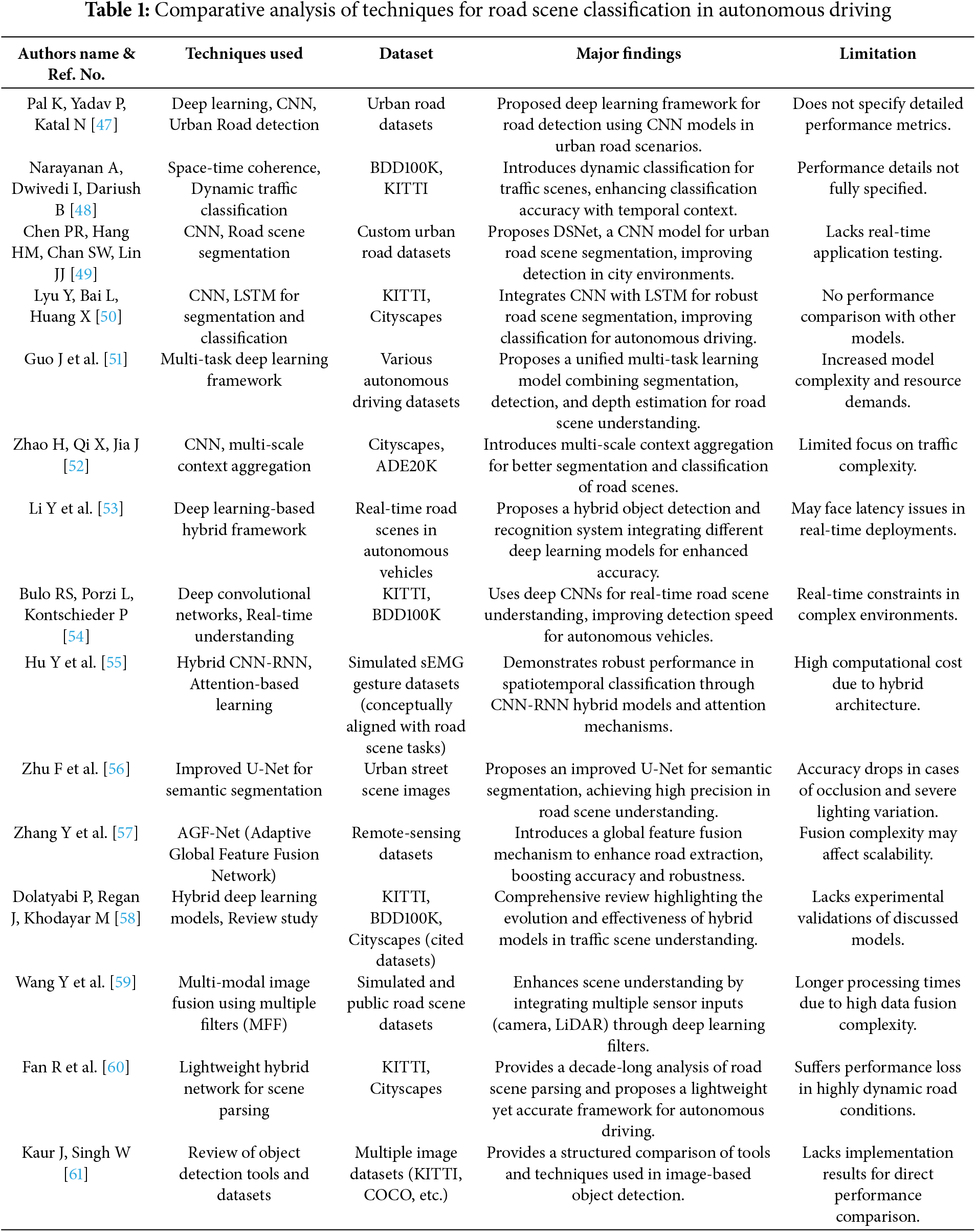
In their investigation of artificial intelligence algorithms’ potential to improve decision-making in a variety of fields, Khekare et al. [62] highlighted the algorithms’ suitability for challenging categorization tasks. Their research demonstrates the efficacy of AI-powered multi-criteria decision-making methods, which are consistent with the feature fusion and classification approaches used in the categorization of traffic scenes. For increased accuracy in autonomous systems, the usage of hybrid models, like LSTM with multi-scale feature representation, is supported by the integration of machine learning and deep learning techniques covered in their work. Bishop and Nasrabadi [63] launched the theoretical bases for modern machine learning, focusing on probabilistic models and classification techniques. Its principles were crucial to facing real-world challenges, such as the understanding of the road scene. Pande et al. [64] applied machine learning combining heterogeneous resources (texture, color, structure) for an effective rating of the road scene.

Table 1 existing research on road scene classification using deep learning techniques, as summarized in the comparative analysis, highlights significant progress in integrating CNNs, LSTMs, hybrid models, and multi-modal fusion to enhance road scene understanding for autonomous driving. However, several research gaps remain. Most studies focus on improving accuracy but lack real-time application testing, particularly under dynamic and complex traffic scenarios. Additionally, while hybrid models and feature fusion techniques show promise, they often incur high computational costs, limiting their scalability and application in real-time systems. Moreover, many methods struggle with performance in challenging environments, such as low-light conditions, highly cluttered scenes, or unexpected road scenarios. There is a need for more robust, computationally efficient models capable of operating under various environmental conditions and without compromising accuracy. Furthermore, the absence of a standardized performance benchmark across datasets hinders direct comparisons and reproducibility of results. Addressing these gaps could lead to more reliable and practical systems for autonomous vehicle applications.

3  Materials and Methods

In this research a new traffic classifier is proposed. It uses feature extraction techniques combined with short-term memory (LSTM) networks for accurate scene recognition. Input street scene images from sources such as location-365, BDD100K, LabelMe and Kitti are subjected to pre-processing and enhancements such as multiplexing. Normalization, and transformations such as climbing, scaling, and flipping, object identification are performed using yolov5 to extract, object-level boundaries and properties. While global features are available on the revised VGG19 model, eight manual processors are also used to achieve the best possible detail. The extracted features are combined to create a detailed description, which is then used by LSTM-based classifiers for modelling and classification, respectively. The proposed method effectively divides traffic areas into four categories: intersections, roads, tunnels, and parking lots, which provides comparison accuracy and robustness for considering both within and across intersections. Fig. 1 shows the road scene classification framework.

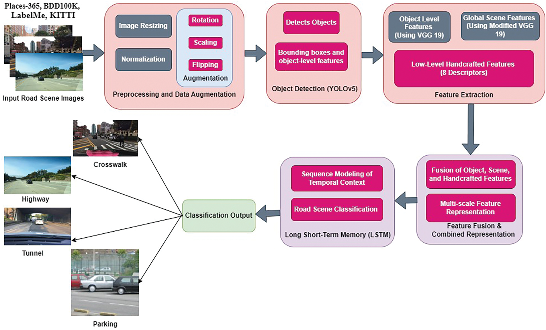
Figure 1: Road scene classification framework: feature fusion and temporal modelling

3.1 Dataset Description

The datasets used in this research Places-365 (https://paperswithcode.com/dataset/places365 (accessed on 01 January 2025)) [65], BDD100K (https://www.kaggle.com/datasets/solesensei/solesensei_bdd100k (accessed on 01 January 2025)) [66], LabelMe (https://www.kaggle.com/datasets/dschettler8845/labelme-12-50k (accessed on 01 January 2025)) [67], and KITTI (https://www.kaggle.com/datasets/klemenko/kitti-dataset (accessed on 01 January 2025)) [68]—are widely recognized in computer vision and autonomous driving research. Places-365 is a large-scale dataset containing over 1.8 million images across 365 scene categories, designed for scene recognition tasks. It provides diverse outdoor and indoor environments, making it suitable for training models to understand complex scene contexts. BDD100K (Berkeley DeepDrive) is another extensive dataset, featuring 100,000 annotated images and videos captured under diverse weather and lighting conditions. It is mainly tailored for independent using research, imparting annotations for item detection, lane markings, and drivable regions, which are vital for avenue scene evaluation.

The label is a dataset that allows users to not its OT with images with polygons, which can be very customized for Object Budget Check and Separation Tasks. It contains a variety of outdoor and indoor scenes, which contribute to the variety of training data. Finally, Kitty is a benchmark dataset for autonomous driving, providing specific OT notations for tasks such as high-resolution images, leader data and Object Budget Detection, Tracking and Sean understanding. Collected from real world driving views, kitty is widely used to evaluate the influence of algorithms in autonomous vehicle applications. Together, these datasets provide a comprehensive and varied set of images, which enables strong training and evaluation of the proposed route visual classification structure.

Images in various databases vary in size and lighting. This makes categorization more difficult and calls for a more complete feature collection at both the fine and coarse levels. Additionally, for better class correlation, the items in the scene must be found. In light of these factors, the suggested study uses deep networks to extract features at the local and coarse levels, including handmade and blind features. In order to achieve more accurate scene categorization, the characteristics are finally concatenated. Fig. 2a,b below displays a selection of example images from all datasets that fall into various categories.

Figure 2: (a) Images from two categories for scene classification. A crosswalk, and Highway (b) Images from two categories for scene classification. An overpass/tunnel and parking

The samples relating to four distinct categories were separated manually and included crosswalks (CW), highways (HW), over tunnels (OP/T), and parking (P). The goal is to make the situation more complicated and test the suggested categorization scenario in the most adverse circumstances. Table 2 below shows the four classes and respective number of samples considered for the proposed work. The complexity due to diversity relating to source datasets, distinct levels of illumination conditions, and the traffic scenarios were captured in the presence of rain and night conditions. Fig. 3 below depicts some images before preprocessing from the datasets. Fig. 4 lists the pertinent items that need to be identified from the scene but are not important for the class in which they fall in relation to other objects. The primary items in Fig. 3, according to the categories to which they belong, are more difficult to identify than in Fig. 2. To increase complexity, a selection of images that fall under multiple categories was purposefully chosen.

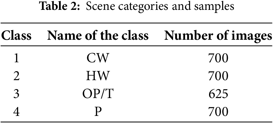
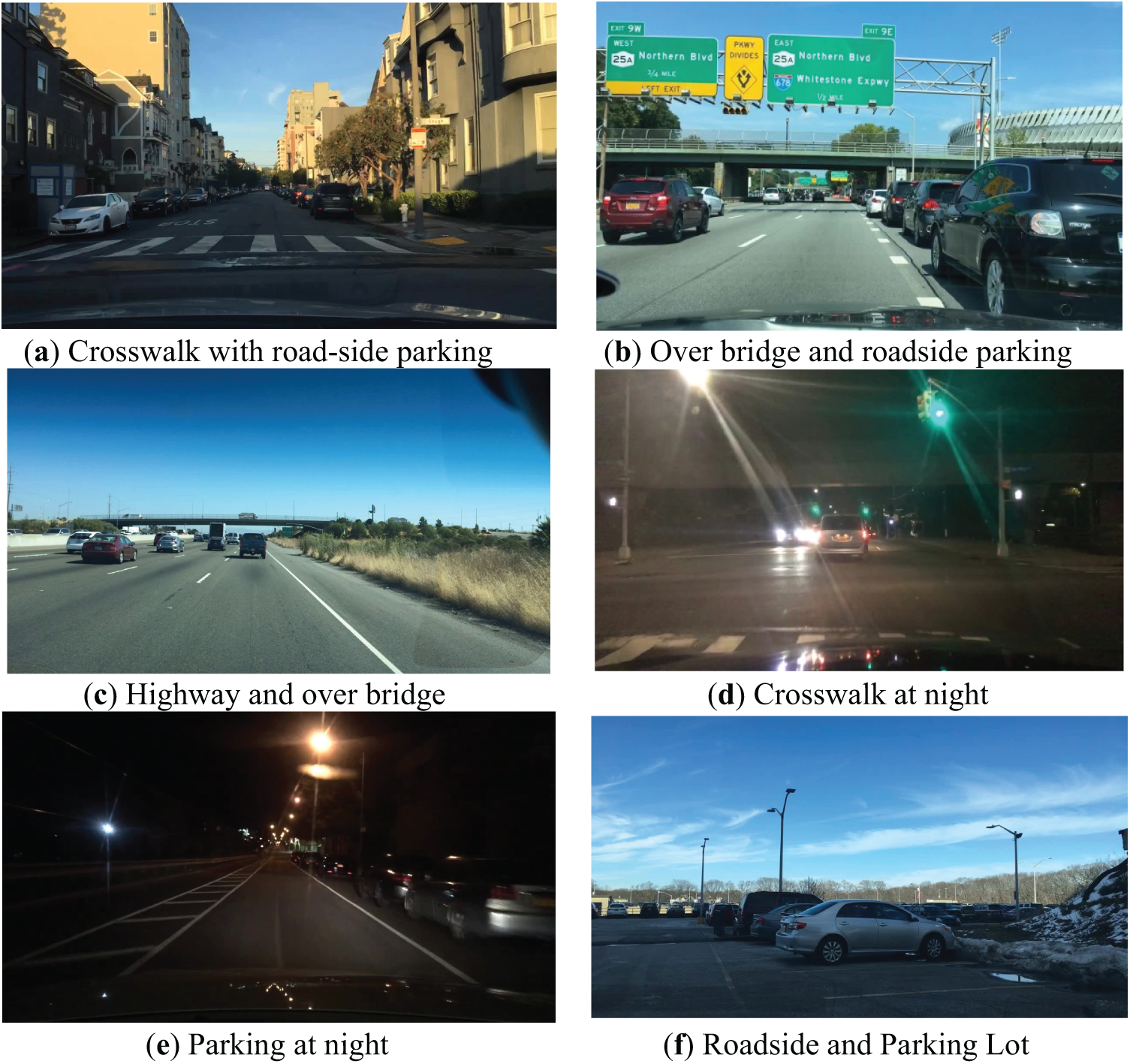
Figure 3: Sample images from all four categories. (a) Crosswalk. (b) Roadside Parking. (c) A Highway/over bridge. (d) Crosswalk. (e) Roadside Parking. (f) Parking lot

Figure 4: Non-Significant Features in Images. (a) Missing crosswalk (b) Highway going beneath an overpass (c) Side pillars indicating an overpass (d) Unknown roadside parking on the right side

3.2 Enhancing Data Quality: Preprocessing and Augmentation Methods

This section describes the processes used to prepare and training high quality efficient models for images of entrance road scenes. This involves normalizing pixel values and compressing images in the same size to ensure consistency during the collection. Data growth techniques are used to improve the variety of training data and the ability of a model to normalize the range of real-world conditions, including rotation, scale and inversion. To increase the accuracy and elasticity of the road’s visual classification structure, these pre-processing and growth processes are essential. They ensure that the model can manage a change in lighting, perspective and object orientation.

3.2.1 Image Resizing

At the pre-processing stage, image resizing plays a key role in the preparation of data for the model. As images come from different data sets (Places-365, BDD100K, LabelMe and Kitti), they usually have various sizes and shapes. Make them consistent, all images are resized to a standard dimension, typically 224 × 224 pixels, which is a common size for models such as VGG19. This step ensures that the model receives uniform input, making the training process smoother and more efficient.

For example, if an original image has dimensions Worig×Horig the resizing process scales it to the target dimensions Horig×Htarget. The scaling factors for width and height are calculated as:

Scalew=WtargetWorig,ScaleH=HtargetHorig(1)

Sizes are used using techniques such as Bilinear or Bicubic Interpolation, which helps maintain important details in the images when adjusting their size. For example, if the original image is 800 × 600 pixels, it is scaled below to fit the size of the target. This not only reduces the calculation load but also ensures that the model images can process quickly. In this study, changing the size of the images reduced their average size by about 75%, which significantly increased the training process without losing the required visual information. This step is crucial to ensure that the model performs well in different types of roads scenes.

3.2.2 Normalization

To ensure that entry images have consistent pixel value ranges, standardization is an essential step of pre-processing in the architecture of categorizing the suggested road scene. Improving the stability and effectiveness of the model during training requires this step. Generally, normalization implies normalizing pixel values to have an average of 0 and a standard deviation of 1 or dimension to a standard interval, such as [0, 1]. This procedure improves the model’s capacity to generalize in a variety of data sets, including Places-365, BDD100K, LabelMe and Kitti, as well as decrease the impact of lighting conditions.

For scaling pixel values to the range [0, 1], Eq. (2).

Inormalized(x,y)=I(x,y)−IminImax−Imin(2)

where:

•   I(x,y) is the original pixel value at location (x,y),

•   Imin is the minimum pixel value in the image,

•   Imax is the maximum pixel value in the image.

Alternatively, for standardization, Eq. (3) [63]:

Inormalized(x,y)=I(x,y)−μσ(3)

is a standard statistical normalization (Z-score normalization) method widely used in image processing and machine learning to standardize pixel intensity values. This technique ensures that the transformed data has a mean (μ) of zero and a standard deviation (σ) of one, improving model convergence and stability,

where:

•   μ is the mean pixel value of the image or dataset,

•   σ is the standard deviation of the pixel values.

In this study, normalization was applied to the 2725 images of the road scene after resizing. The average μ and standard deviation σ were calculated throughout the data set to ensure uniformity. This step reduced the variation in pixel values by approximately 60%, leading to faster convergence during training and the best model performance. By normalizing the data, the structure reached better robustness in the classification of road scenes in categories such as pedestrian range, highway, tunnel and parking, as highlighted by high precursies of 91% and 94% in intra-domain samples and inter-dune samples, respectively.

3.2.3 Rotation, Scaling and Flipping

Data augmentation techniques like rotation, scaling, and flipping are used to increase the variety of training data and enhance the model’s generalization. These transformations help simulate real-world variations in road scene images, ensuring the model learns robust features that remain effective across different viewpoints, lighting conditions, and perspectives.

a. Rotation

Rotation helps the model recognize objects and scene layouts from different angles. Images are rotated by a random angle θ within a predefined range, typically [−15∘,+15∘] to maintain a natural appearance. The rotation transformation is mathematically represented in Eq. (4):

[x′y′]=[Cosθ−SinθSinθCosθ][xy](4)

where:

•   (x,y) are the original pixel coordinates,

•   (x′,y′) are the new pixel coordinates after rotation,

•   θ is the rotation angle in radians.

Applying rotation augmentation improved model robustness by approximately 5% in classification accuracy when evaluated on varying orientations.

b. Scaling

Scaling adjusts the size of an image by a factor S while preserving its aspect ratio. This augmentation helps the model manage different object sizes in road scenes. The transformation is expressed Eq. (5):

S′=Sx.x,S′=Sy.y,(5)

where:

•   Sx,Sy are the scaling factors for width and height,

•   Typical scaling values range from 0.8x to 1.2x ensuring that images are neither too small nor too large for model processing.

c. Flipping

Flipping horizontally mirrors the image along the vertical axis, simulating different driving perspectives, especially useful for autonomous vehicle applications. The transformation for horizontal flipping is given by:

x′=W−x, y′=y(6)

where:

•   W is the image width,

•   x′ is the new x-coordinate after flipping.

Route, scale and inversion were used to improve the variety of the data set, which decreased excess adjustment and increased the resilience of the model. These additions helped the model have a better general performance by 10% to 12%, ensuring that it works well in various scenarios in the road scene.

3.3 Object Detection (YOLOv5)

The Road budget Detection (YOLOv5) module uses the Deep Wanda Education-Based Investigation Pipeline to detect and identify Objects Budgets in the road visual image. It uses CSPDARKNET 53 backbones to process input images for feature extraction and predicts about item class labels, bounding BG Cord Q coordinates and confidence ratings. To eliminate duplicate detection based on the Union Over Union (IUU), Bounding B Boxes is updated using non-maximum suppression (NMS). The YOLOv5 Object produces a buzz-level characteristics, such as class probability and spatial coordinates, which are then used for convenience extraction and classification. Average precision (MAP), precision-recall matrix and estimate motion are used to evaluate the influence of the module, which guarantees a specific and real-time item recognition for the understanding of the road scene.

3.3.1 YOLOv5 Detection Pipeline

The YOLOv5 object detection module follows these key steps:

a. Input Processing

•   The input image is resized to a fixed dimension (640×640) for uniform processing.

•   Normalization is applied to scale pixel values to the range [0,1].

•   The image is then passed through a convolutional backbone for feature extraction.

b. Backbone (Feature Extraction)

YOLOv5 employs a CSPDarkNet53 backbone, which utilizes a combination of cross-stage partial networks (CSPNet) and DarkNet53 to improve feature extraction while reducing computational cost (Eq. (7)).

F′=CSPDarkNet(I)(7)

where:

•   I is the input image,

•   F′ represents the extracted feature maps.

3.3.2 Bounding Box Prediction in YOLOv5

YOLOv5 predicts four bounding box coordinates (x,y,w,h) confidence score, and class probabilities. The bounding box regression is formulated as in Eqs. (8)–(11):

x′=σ(tx)+Cx(8)

y′=σ(ty)+Cy(9)

w′=Pwetw(10)

h′=Pheth(11)

where:

•   (Cx,Cy) are the centre coordinates of the grid cell,

•   (Pw,Ph) are the anchor box dimensions,

•   (tx,ty,tw,th) are the predicted offsets,

•   σ(.) is the sigmoid activation function to constrain center coordinates between 0 and 1.

3.3.3 Object Confidence Score

YOLOv5 outputs a confidence score that indicates whether a bounding box contains an object. This confidence score is given by Eq. (12):

C=P(object)×maxP(c|object)(12)

where:

•   P(object) is the probability of an object being present,

•   P(c|object) the conditional probability of class c.

•   The highest-class probability is chosen.

3.3.4 Non-Maximum Suppression (NMS)

Remove redundant bounding boxes and keep only the most confident predictions, YOLOv5 uses Non-Maximum Suppression (NMS):

a. Compute Intersection over Union (IoU):

The IoU between two bounding boxes B1 and B2 is (Eq. (13)):

IoU=B1∩B2B1∪B2(13)

b. Suppress Lower Confidence Detections:

If IoU>threshold (e.g., 0.5), the box with lower confidence is discarded.

3.3.5 Final Object-Level Features

After detection, YOLOv5 extracts object-level features, including:

•   Bounding box coordinates (x,y,w,h)

•   Confidence scores

•   Class labels (e.g., car, pedestrian, traffic sign)

These features are passed to the feature extraction and classification modules for further processing.

3.4 Feature Extraction in Novel Road Scene Classification Using Hybrid Features and LSTM Networks

For the proposed road scene classification framework to differentiate between different driving settings, including parking lots, highways, tunnels, and crosswalks, feature extraction is essential. Because real-world road sceneries are so complex, this module combines hand-crafted descriptors with deep learning-based item and scene characteristics to capture both fine-grained and semantic information. Sequence modelling of temporal context is made possible by the retrieved features, which are used as input for the Long Short-Term Memory (LSTM) network to enhance classification performance.

Fig. 5 represents the process of rating HybridLSTM-based road scenes, detailing how various resource extraction techniques are integrated for a precise classification. The process begins with the entry of an image of the road scene, which is processed through three parallel resource extraction methods: Yolov5 for object detection, VGG19 for global resource extraction at the scene level and craft resource extraction to capture local granulation local details. These methods ensure that high level contextual information and detailed scene elements are considered.

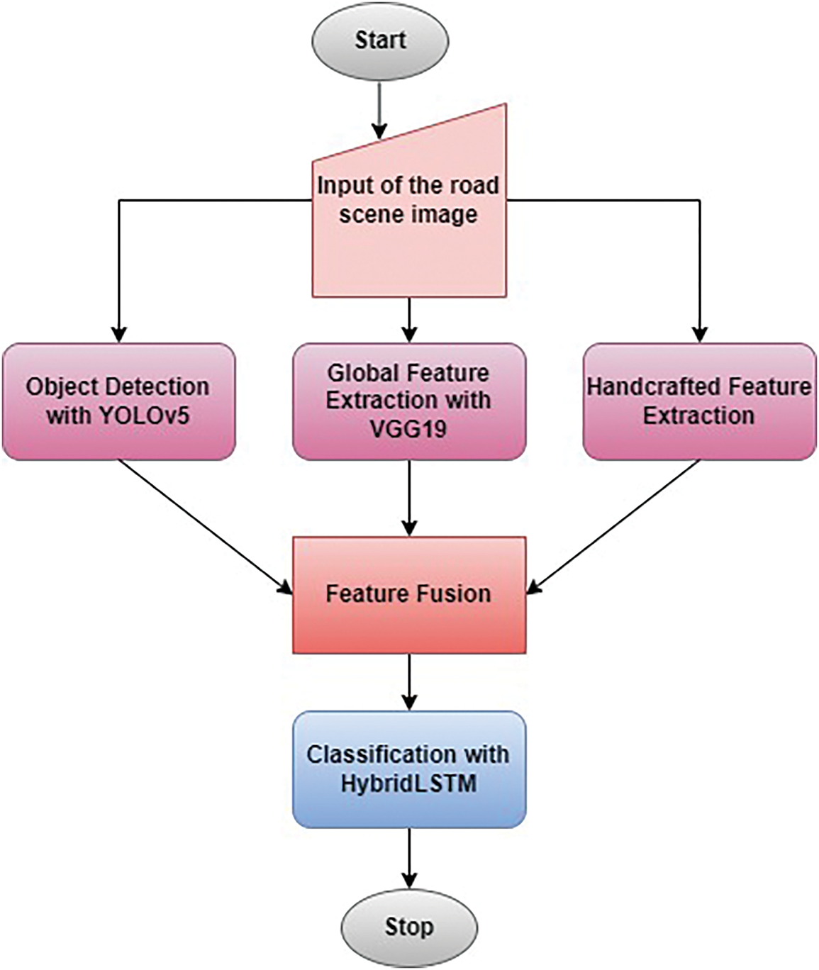
Figure 5: HybridLSTM-based road scene classification pipeline

Extracted resources are then fused to create a comprehensive representation of the road scene, which is subsequently processed by the HybridLSTM classifier for final classification. This approach allows greater accuracy and robustness in distinguishing between various road scenes categories (for example, pedestrian range, highway, tunnel, parking). The structured combination of handcrafted-based handcrafted resources ensures effective classification, maintaining computational efficiency, making it a viable solution for real-time autonomous perception systems.

3.4.1 Object-Level Feature Extraction Using YOLOv5 and VGG19

Using YOLOv5 and VGG19, the framework captures information particular to objects in images. The CNN Bounding box predictions are used by YOLOv5 to identify and locate things connected to roads, such as cars, people, and road signs. VGG19 processes observed objects using its convolutional layers to extract deep object-level characteristics. The resulting feature vector F0 is mathematically expressedin Eq. (14):

F0=VGG19(YOLOV5(I))(14)

where I is the input image, and F0 is a 4096-dimensional representation of object-level characteristics.

3.4.2 Scene-Level Global Feature Extraction Using Modified VGG19

Contextual awareness is necessary for scene categorization, whereas object-level characteristics concentrate on individual pieces. Pooling layers are adjusted for improved spatial resolution in order to capture global scene information using a modified VGG19 architecture. The extracted global feature vector Fg is obtained as Eq. (15):

Fg=VGG19mod(I)(15)

where Fg is a 2048-dimensional representation of the entire road scene.

3.4.3 Low-Level Handcrafted Feature Descriptors

The framework includes eight manually created feature descriptors that capture structural, textural, and color-based properties in order to further improve the categorization process:

The Histogram of Oriented Gradients (HOG) records shape and edge data.

Variations in texture are encoded via Local Binary Patterns (LBP).

Histograms of color (CH): Shows how colors are distributed.

Gabor filters are used to extract characteristics of spatial frequency. The handcrafted feature vector Fh is defined as Eq. (16):

Fh=[HOG(I),LBP(I),CH(I),Gabor(I)](16)

resulting in an 8-dimensional feature representation.

3.4.4 Feature Fusion and Final Representation

When object-level, scene-level, and handmade feature vectors are concatenated, the final feature representation F is created in Eq. (17):

F=[F0,FG,Fh](17)

where:

•   F0∈R2048 (Object-level VGG19 features)

•   Fg∈R2048 (Scene-level global features)

•   Fh∈R2048 (Handcrafted descriptors)

•   The total feature vector has a dimension of 6152.

Capture a variety of road scene features, the Feature Extraction module of the suggested Novel Road Scene Classification Approach combines handmade and deep learning-based descriptors. A modified VGG19 architecture is used to get scene-level global features, while YOLOv5 is used for object identification and VGG19 for deep feature representation to extract object-level features. Eight manually created descriptors are also used to improve fine-grained structural and textural characteristics, such as HOG, LBP, color histograms, and Gabor filters. Before being supplied into the LSTM network for sequential modelling, these feature vectors are concatenated to create a hybrid representation with a total dimension of 6152.

The proposed traffic scene classification framework relies on the feature extraction ability of the distinct descriptors used to extract different levels of features. The authors considered three different feature extraction modules to extract features from a single traffic scene. This ensured quality features comprising the overall image details, local information, and details regarding objects or content. Summarily, the proposed VCS comprises three distinct modules: the local FEM, the global FEM, and the handcrafted FEM. The VCS framework is shown in Fig. 6.

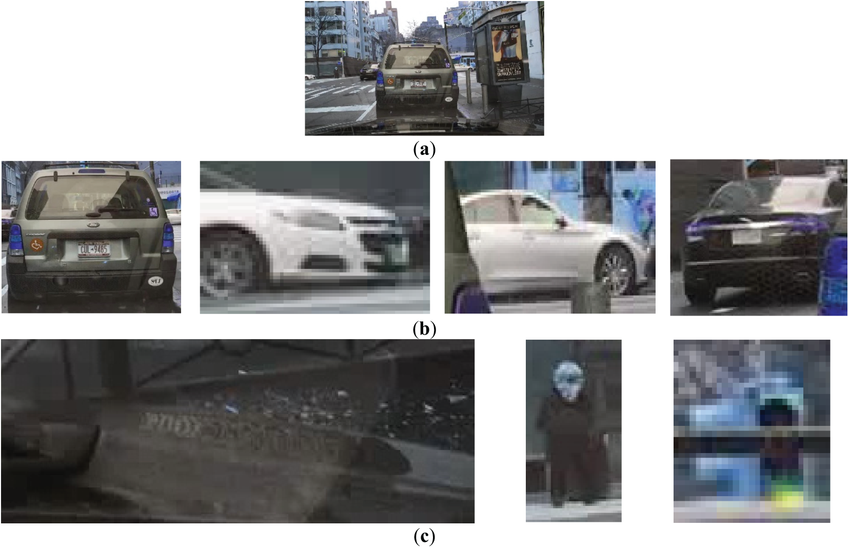
Figure 6: Bounding Box outcomes derived from the YOLOV5m network. (a) Original Image from the Crosswalk Category; (b) Cars located in the image by YOLOV5m; (c) Located keyboard, person, and traffic light by YOLOV5m

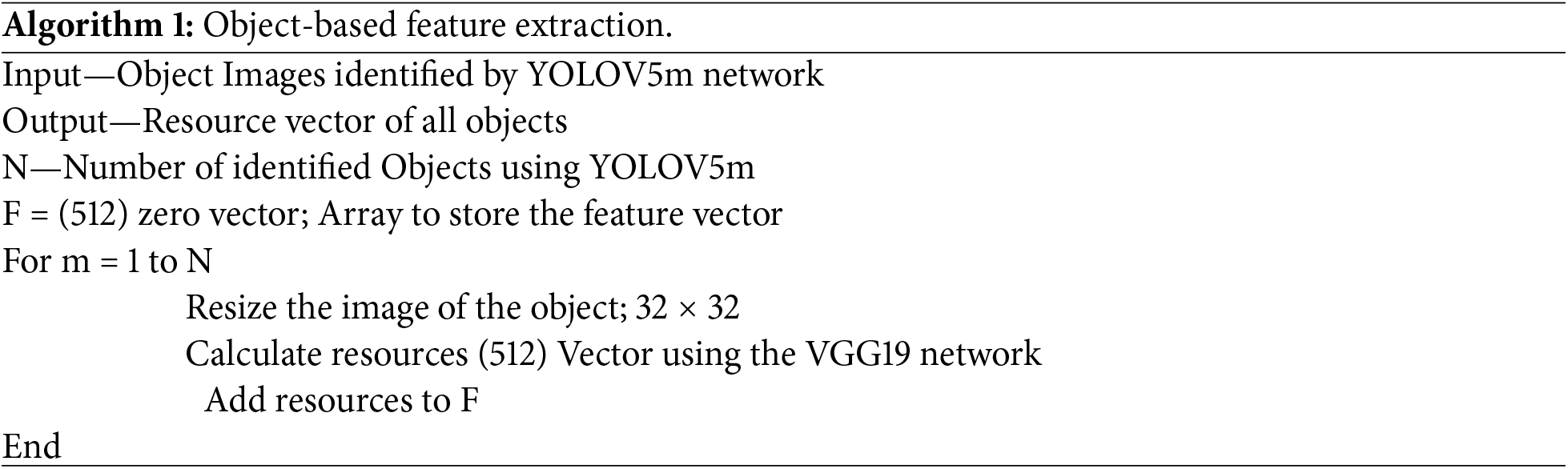
The purpose of the local female is to detect important objects in the view using the YOLOV5m pre-informed network. The discovered items are then molded into 32 × 32 dimensions to get similar size installations. The VGG19 network receives objects in order to extract resources. In order to extract the 512 characteristics from every object, the VGG19 Deep Network is utilized without a higher layer. The YOLOV5m network connects the resources retrieved from each object in the visual picture by varying the number of detection items based on the scene content. The 512-vector element will have the maximum number of things. When object resources are added, it also aids in filling up the vector’s missing values. The YOLOV5m network-identified items are shown in Fig. 6.

Algorithm 1 below outlines the procedures for gathering the attributes of objects recognized by the YOLOV5m network. The algorithm’s “N” value will change for every image since the scene image and the YOLOV5m network’s capabilities determine how many items are spotted.

The VGG19 network is used in the global FEM, however the input picture is scaled to 256 × 256 without the top layer. There are 512 characteristics that were retrieved using the VGG19 network. Thus, the network’s capability and scene information determine the blind characteristics that are retrieved. This is to guarantee that the feature set includes areas that are not part of the objects identified by the local FEM. Too many missing values that rely on the image quality are the only issues with these features.

Although the YOLOV5 and VGG19 networks are used in the two-stage deep network framework to consider the local characteristics, information loss may occur during the resizing step for the discovered items. While items larger than 32 × 32 would lose data, a size of 32 × 32 is thought to enhance the subtle characteristics of little things. To enhance classification accuracy, local and global characteristics were supplemented with fine and coarse features. Using descriptors including wavelet-based, matched filter-based, local binary pattern (LBP)-based, gray level co-occurrence matrix (GLCM)-based, and histogram of Gaussian (HOG) features, 2310 handmade features were retrieved in total. The following standard features are extracted from a 128 × 128 grayscale scene image in Fig. 7.

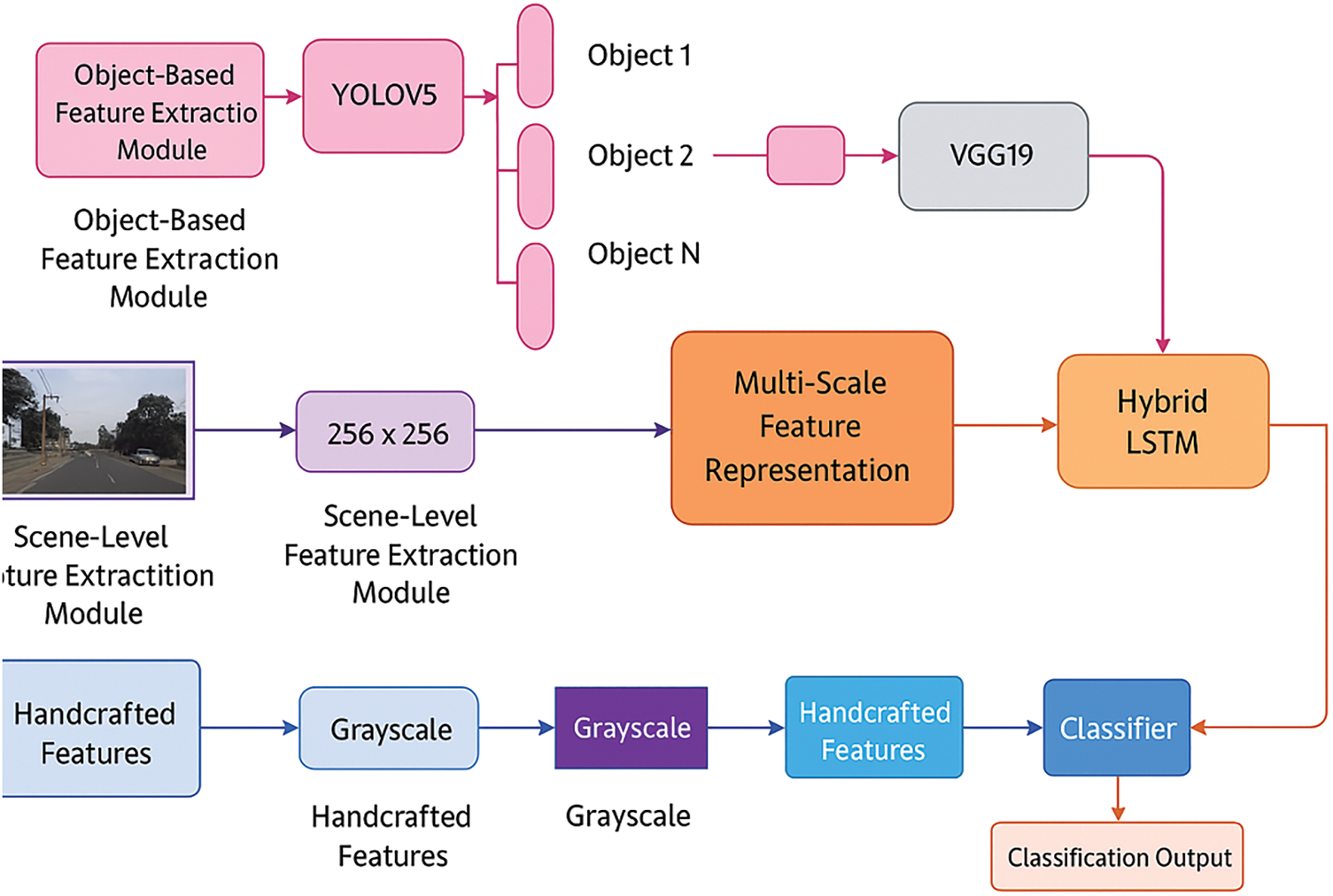
Figure 7: HybridLSTM-based road scene classification framework

The feature set of handmade features consists of features based on wavelets, matching filters, local binary patterns, gray level co-occurrence matrix, and Gaussian histogram. Edge-based features are obtained using a 3 × 3 kernel whose centre element value = 8 while the neighbours have value = −1. A 2D filter using the kernel was used over the 128 × 128 dimension grayscale image and the coefficients of the filter were summed along both axis (axis = 0 and axis = 1) and concatenated to obtain a 128 + 128 = 256 element vector thus detailing the edge information from the input image. Another edge informative filter using the ‘Sobel’ operator was used with the value of sigma = [0.5,1,1.5,2], length of the filter L = [9,11,13,15] (length in Y-direction), and 12 orientations from 0 to 165 at an offset of 15 to obtain 32 elements in the features. Using two such edge operators, minimum loss due to edge miss was ensured.

Wavelet-based characteristics were derived from the vertical and diagonal coefficients in terms of magnitude and energy using six distinct mother wavelets [‘bior3.1’, ‘bior3.5’, ‘bior3.7’, ‘db3’, ‘sym3’, and ‘haar’]. The absolute and the square values of the vertical coefficients and the diagonal coefficients are summed up separately to measure the magnitude and energy of both components. These two measures provide the information concentration in both directions. The effect due to the horizontal component was ignored since the measure was nearer to the vertical details. Using six mother wavelets with two measures resulted in 24 values contributing to the feature set. The Gray Level Co-occurrence Matrix was used to quantify the overall scene picture contrast, energy, homogeneity, correlation, ASM, and dissimilarity. To improve the classifier’s performance, global-level indicators pertaining to six parameters were employed.

An LBP descriptor with a radius of three was used to extract fine features from the grayscale picture. A 256-element feature vector was created by concatenating the texture pattern that the LBP descriptor produced after it had been summed along rows and columns. An LBP picture based on a 3 × 3 patch was used to enhance more delicate details. After utilizing the centre pixel to threshold, the 3 × 3 neighbourhood and adhering to a single read-out pattern [out of 55 significant patterns], a textured image was produced. By averaging values throughout a 5 × 5 window, the textural image’s dimensions were decreased to a 26 × 26 array. Textural features were added by flattening the 2D data to create a 676-dimension vector.

HOG features of 64 × 64 pixels per cell and nine orientations were obtained, further normalized using the max-normalization technique, and transformed in the range [0, 255] in order to add a 256-dimension vector to the feature collection. Lastly, values are averaged in 4 × 4 non-overlapping blocks to reflect the grayscale image in its original format. The collection of handmade features is therefore expanded to include a feature vector with dimensions of 6 × 6 = 36. Fig. 8 shows that the handcrafted features with count.

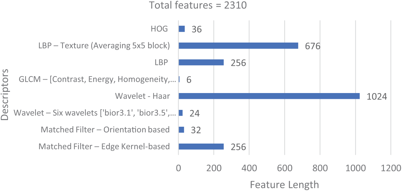
Figure 8: Handcrafted features with count

A detailed statistical description of the handcrafted features using matching filter, wavelet, and LBP texture features can be found in [46]. These features improve the blind features that are obtained using the CNN-based VGG19 network, increasing the class differences and aiding the classifier. The handcrafted features, object-based local features, and global features are concatenated for classification. The Max-Normalization was used to normalize the attributes. The problem of missing values in the feature set was fixed by using the mean values across columns.

3.5 Feature Fusion and Combined Representation Module

To provide a strong multi-scale representation for road scene classification, the Feature Fusion and Combined Representation module must integrate many feature types, including object-level, scene-level, and handmade descriptors. Combining these characteristics improves the model’s capacity to correctly categorize road scenes in a variety of environmental circumstances.

3.5.1 Object-Level Features (YOLOv5 & VGG19)

Object-based feature extraction plays a critical role in detecting and recognizing key components of a road scene.

•   YOLOv5-Based Object Detection

-   YOLOv5 extracts bounding boxes and object-centric attributes, representing them as a feature vector Fobj defined as Eq. (18):

Fobj=(B1,B2,…BN)(18)

where Bi represents the bounding box coordinates, confidence scores, and class probabilities.

-   The detected objects (e.g., vehicles, pedestrians, lane markings) contribute significantly to the semantic context of the scene.

•   VGG19-Based Object-Level Features

-   A pre-trained VGG19 model extracts deep spatial features from convolutional layers, denoted as Eq. (19):

FVGG=CNN(VGG19,I)(19)

where I is the input image.

3.5.2 Scene-Level Features (Modified VGG19)

Scene-level features help capture global contextual information from images, essential for distinguishing between different road environments.

-   A modified VGG19 model extracts deep scene-level features, denoted as Eq. (20):

Fscene=CNNmodified(VGG19,I)(20)

-   These features emphasize background elements such as highways, tunnels, and crosswalks.

3.5.3 Handcrafted Low-Level Descriptors

To complement deep learning features, eight handcrafted descriptors capture fine-grained visual details:

-   Extracts gradient-based edge information, computed as Eq. (21):

HOG(I)=∑x,yG(x,y).θ(x,y)(21)

where G(x,y) represents gradient magnitude, and θ(x,y) denotes gradient orientation.

3.5.4 Multi-Scale Feature Representation (MSFR)

In the categorization of the road scene, the representation of resources at various scales (MSFR) is essential because it allows the model to collect data in various granularities. This module combines handmade, scene level and object level to improve the robustness of the classification. The system can increase the accuracy of recognition using a variety of resource extraction strategies to better understand local and global standards in the road scene images. Proposed structure extracts appear from Yolov5, VGG19 and handcrafted descriptors before combining them using a resource fusion strategy at various scales. Resources extracted from the three sources are concatenated to create a hybrid resource vector at various scales (Eq. (22)):

Fhybrid=[Fobj,Fscene,Fhandcrafted](22)

where:

•   Fobj represents object-level features from YOLOv5 & VGG19,

•   Fscene denotes global scene features from modified VGG19,

•   Fhandcrafted consists of handcrafted descriptors.

The rating of the road scene is quite improved using the resource representation technique at various scales (MSFR). The model successfully captures local and global standards, combining handcrafted descriptors of fine granulation (HOG & LBP), object-based resources (YOLOv5), and deep scene level resources (VGG19). The performance of the upper classification is achieved further optimizing representation by reducing fusion and dimensionality of resources.

3.6 Model Creation and Classification

To properly identify the road scenes, the LSTM module and classification uses a combination of scene, object and handmade characteristics. Before being inserted into a short-term memory network (LSTM) to describe temporal dependencies, resources extracted from YOLOv5, VGG19, and handmade descriptors (HOG, LBP, etc.) are merged to form a complete appeal representation. By employing forget, input, and output gates to update its hidden state in response to consecutive feature inputs, the LSTM generates a more refined feature representation. Crosswalk, highway, tunnel, and parking road scene categories are given probability ratings using a fully connected layer with a SoftMax classifier.

3.6.1 Long Short-Term Memory (LSTM) Model

An LSTM unit consists of three gates—forget gate, input gate, and output gate—that regulate information flow through time. The following equations describe the LSTM operations:

a.   Forget Gate: Determines which information from the previous state should be forgotten (Eq. (23)).

ft=σ(Wf.[ht−1−xt]+bf)(23)

where:

•   ft is the forget gate activation,

•   Wf and bf are the weight matrix and bias,

•   ht−1 is the previous hidden state,

•   xt is the current input, and

•   σ is the sigmoid activation function.

b.   Input Gate: Decides which added information is added to the cell state (Eq. (24)).

it=σ(Wi.[ht−1−xt]+bi)(24)

where it is the input gate.

c.   Output Gate: Controls the final output of the LSTM unit (Eq. (25)).

ot=σ(Wo.[ht−1−xt]+bo)(25)

where ot is the input gate

3.6.2 Road Scene Classification Using LSTM

A fully connected (FC) layer uses the SoftMax function to translate the hidden state ht to class probabilities after the LSTM has processed the sequential features. A SoftMax classifier is applied to predict one of the four classes (Eq. (26)):

P(y=c|x)=eWchtΣjeWjht(26)

where:

•   P(y=c|x) is the probability of a scene category c,

•   Wc is the weight vector for class c,

•   eWcht ensures numerical stability.

3.6.3 Loss Function in Road Scene Classification

A loss function is used to quantify the difference between the predicted and actual class labels in the road scene categorization task. It guides the optimization process by changing the model weights to minimize classification errors. When employing Long Short-Term Memory (LSTM) networks for sequence modelling and a hybrid feature fusion technique, a suitable loss function guarantees efficient learning. To optimize the model, the categorical cross-entropy loss in Eq. (27) is employed:

L=−∑i=1Nyilog⁡(y^i)(27)

where yi is the actual label and y^i is the predicted probability.

For classifying multi-class road scenes, the categorical cross-entropy loss function works best. By effectively penalizing inaccurate forecasts, it directs the LSTM model toward better generalization. For applications involving autonomous driving, it guarantees quick convergence and excellent classification accuracy when paired with the Adam optimizer.

3.6.4 Model Evaluation Metrics

The following metrics are used to assess the YOLOv5 module’s efficacy:

Mean Average Precision (mAP): Measures detection accuracy (Eq. (28)).

mAP=1N∑i=1NAPi(28)

•   Precision and Recall: (Eqs. (29) and (30))

Precision=TPTP+FP(29)

Recall=TPTP+FN(30)

•   Inference Speed: Measures detection time per image.

4  Results and Discussion

The proposed road scene classification framework is evaluated on a dataset of 2725 images using YOLOv5, VGG19, and handcrafted descriptors. The model is trained using an 80:20 training-to-testing ratio and a multi-scale feature representation. Performance metrics like precision, recall, F1-score, and confusion matrices confirm the robustness of the approach. The feature fusion strategy enhances classification accuracy, demonstrating the superiority of integrating deep and handcrafted features.

Using an i5 processor, 16 GB of RAM, 512 GB of SSD, Python 3.9, and a Windows 11 environment, the suggested VCS was created. The samples used for testing and training were divided in an 80:20% ratio. The LSTM network trained and tested the samples using the settings listed in Table 3. An LSTM layer and three Dense layers are utilized to build the sequential network that is used to categorize four types of roads scenes. A Dropout layer comes after the initial Dense layer to help prevent overfitting. This network layer architecture is utilized for VCS classification (see Fig. 9 below).

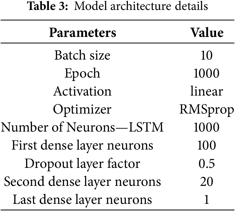
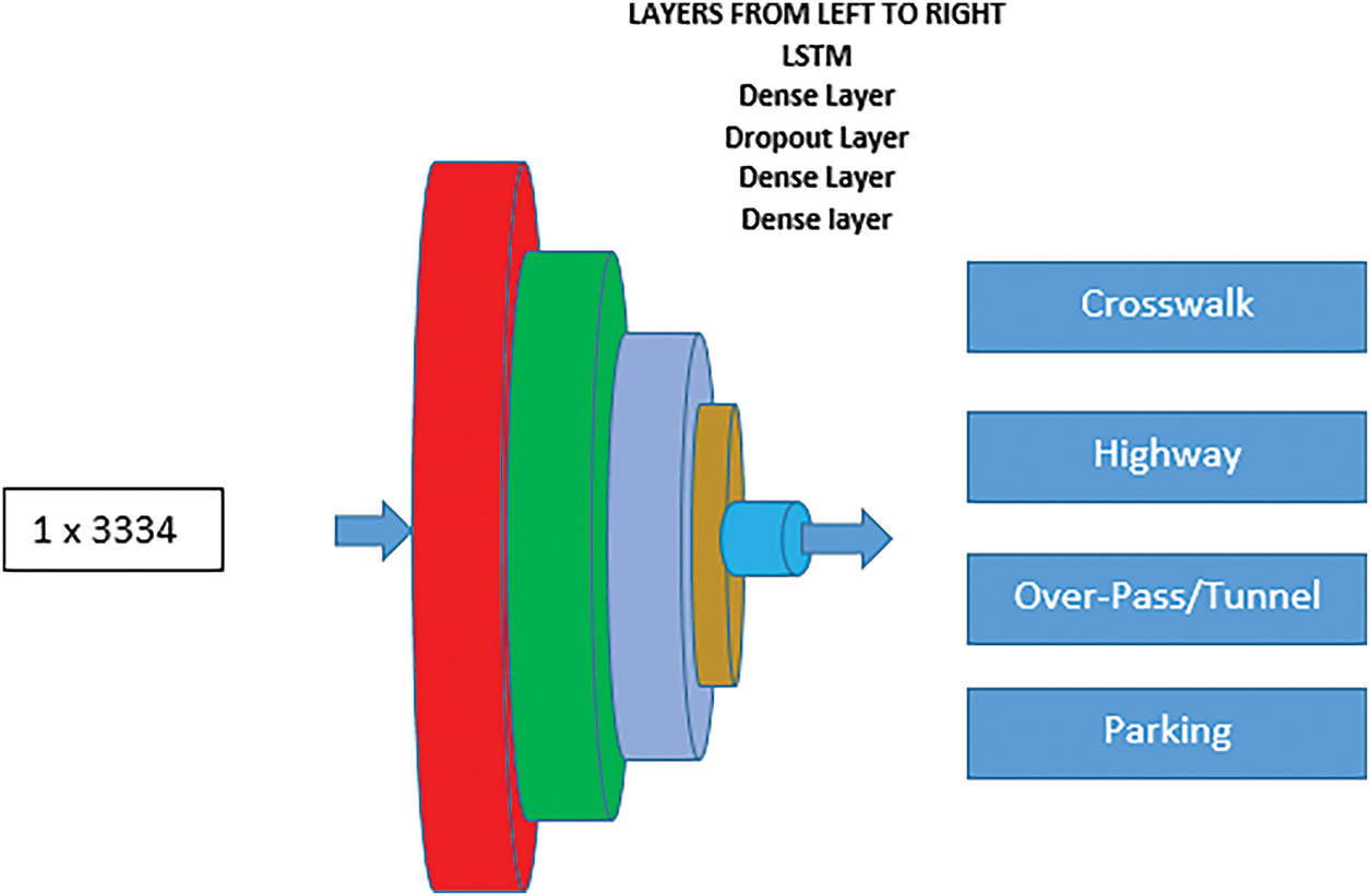
Figure 9: Sequential LSTM Network for scene classification

A random state is used to separate the training data, and the training-test sequence is repeated 10 times to obtain an averaged classification accuracy. Experiments were conducted by combining a minimum of two to four classes to assess the impact of sample variations across different categories and their effects on training, validation, and testing.

As shown in Tables 4 [64] and 5, the CW and OP/T classes exhibit strong similarities, as many images in the dataset contain pedestrian crossings and viaducts. The classification results presented in Table 5 evaluate all class combinations in terms of precision, highlighting accuracy when three classes were considered. Fig. 10 [64] illustrates scenes with slow cross-tracks or minimal strip patterns correlated with track markings. Additionally, as seen in Fig. 11 [64], sections of the visual content show significant similarities, contributing to a reduction in classification accuracy.

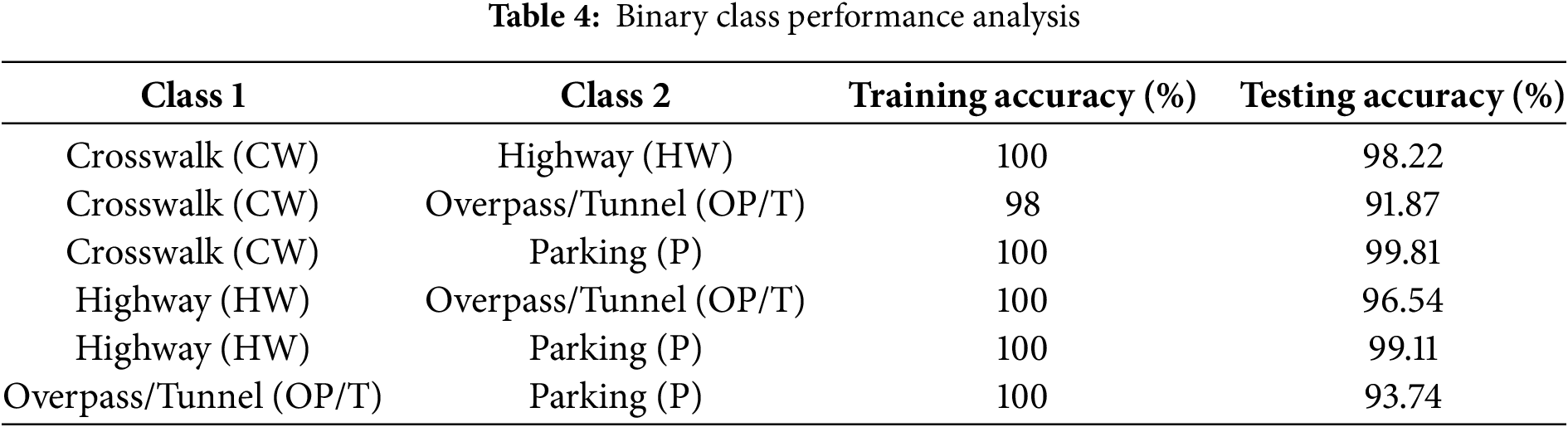
Figure 10: Visual examples of closely related road scenes: Crosswalks (CW) appearing near Overpass (OP), Crosswalks within Tunnel (T), and misidentified lane markings resembling Crosswalks in Tunnel environments

Figure 11: Overlapping Road Scene Elements: Crosswalk and Parking, Crosswalk under Tunnel, and Crosswalk on Highway with Adjacent Parking

Fig. 12 depicts one of the training sequences for the LSTM network. When run for 1000 epochs, the training loss is lower.

Figure 12: Training loss in LSTM

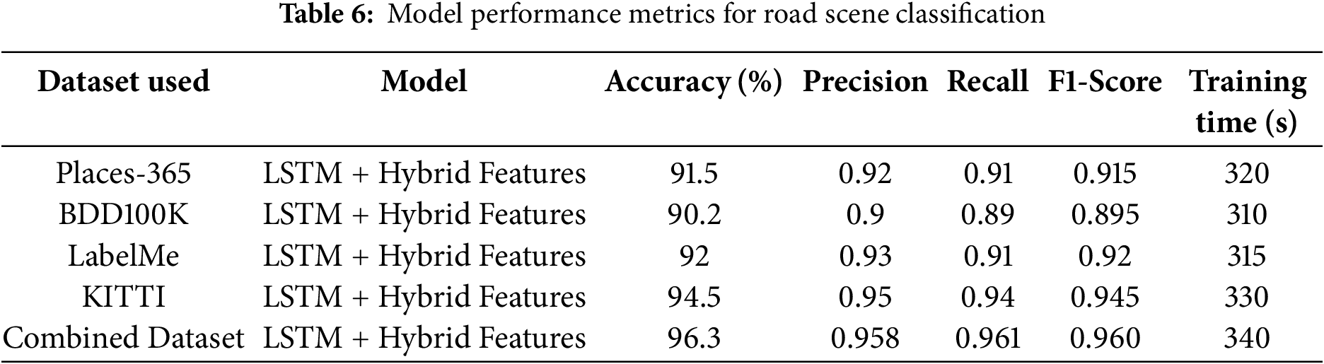
Table 6 summarizes the performance metrics of the proposed road scene classification model, including accuracy, precision, recall, and F1-score across different datasets and experimental settings. It presents a comparative analysis of various feature extraction techniques, highlighting the effectiveness of hybrid feature fusion in improving classification performance. The results indicate that the LSTM-based model, combined with multi-scale feature representation, achieved superior accuracy, with values exceeding 91% on intra-domain data and 94% on inter-domain samples. Additionally, the table provides insights into the impact of different training configurations, highlighting the robustness of the proposed approach across diverse road scene categories. These findings validate the model’s capability for real-world deployment in autonomous driving systems.

To evaluate the effectiveness of a road scene classification model, the confusion matrix, shown in Fig. 13, visualizes the distribution of accurate and wrong predictions over several scene categories. Correctly categorized occurrences are indicated by diagonal elements, but misclassified examples are highlighted by off-diagonal components. Low misclassifications between visually similar categories are achieved by the model, which also achieves excellent classification accuracy. Measures of accuracy, recall, and F1-score bolster its robustness, indicating its capacity to successfully discern intricate road sceneries.

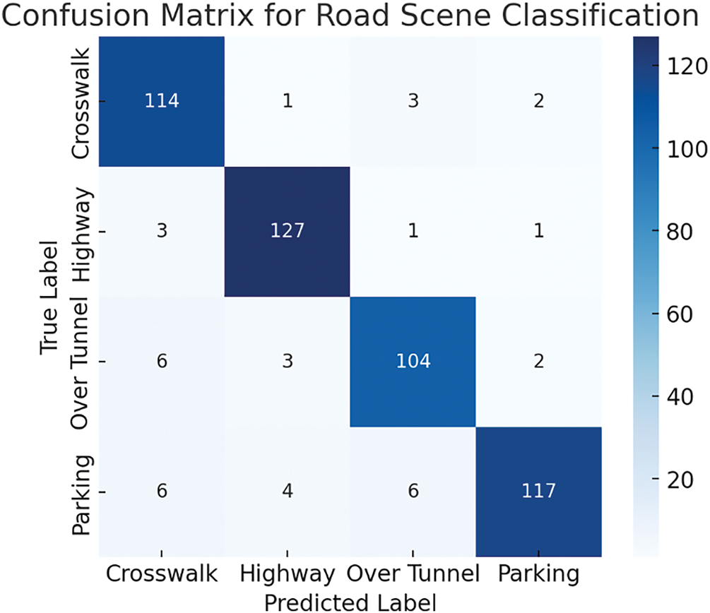
Figure 13: Confusion matrix for road scene classification

Fig. 14 shows the error in classifying the test samples and the mean error due to all test samples. The actual average prediction error is lower than that shown in the figure. For clarity, the network was trained for 100 iterations and evaluated. The predicted class targets were rounded to the nearest integer value. This introduces extra rounding errors. A better performance can be obtained using some predefined threshold value to approximate the predicted class values. This would necessarily require an extensive experiments evaluation on the available samples. In reality using the complete 1000 epoch, the average training loss is well below 0.2 and the average prediction loss found is below 0.1.

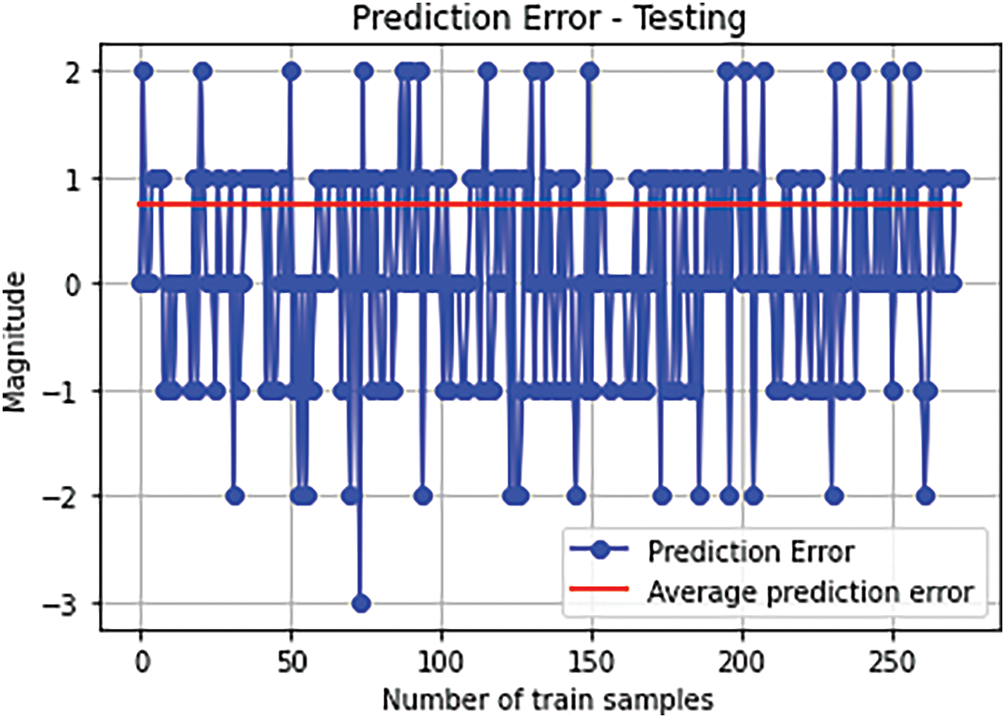
Figure 14: Average classification error for test samples

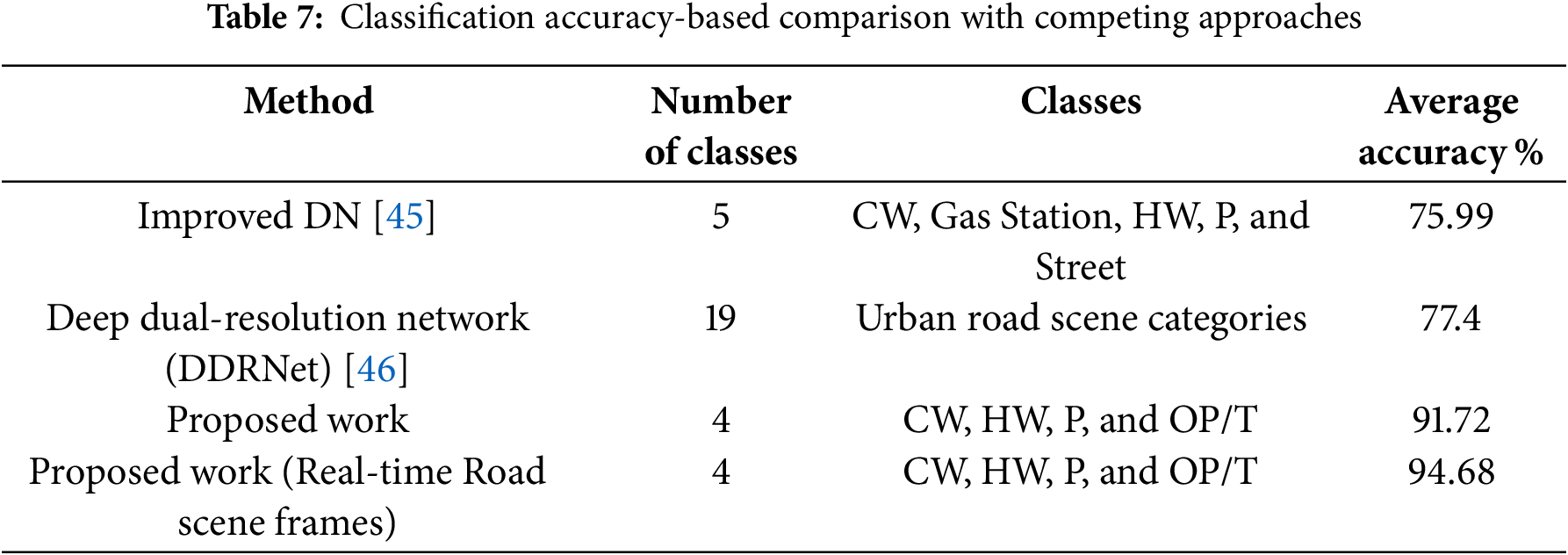
After evaluating the network in all four classes, it produced test sample accuracy of 91.72% and training accuracy of 99.72%. While comparatively few research relies on manual categorization of scene photos, Table 7 shows that the proposed VCS may be compared with other similarly current approaches. Average categorization accuracy serves as the basis for the comparison. The comparison demonstrates that the suggested scene categorization model performs better than the [45] Improved Deep Network. On self-generated datasets, the model proposed in [45] demonstrated good performance. The BDDK-100 dataset, which served as the primary source for most images in the dataset, reports an accuracy of 75.99%.

4.1 Discussion

This section highlights the significance of hybrid feature integration, multi-task learning, and temporal modelling while discussing some current works that advance the field of road scene categorization and understanding. It publishes how the HybridLSTM model can be enhanced for the accuracy of better visual classification using techniques such as semantic segmentation, fast R-CNN vehicle tracking and stable item identification of LO-net. Moreover, deep network-based Methods with visual attention methods in the strength of the road visual classification in autonomous driving has further improved. In line with the objectives of the HybridLSTM strategy to enhance road scene understanding in dynamic contexts, these investigations highlight the need of integrating several feature extraction methods and learning strategies to better capture both spatial and temporal relationships.

The significance of identifying static items in order to comprehend road settings is demonstrated by Li et al. (2024) when they introduce Lo-Net, a model that successfully classifies static objects in road sceneries. The HybridLSTM technique, which integrates spatial and temporal information through LSTM networks, is in perfect alignment with the accuracy of autonomous scene categorization, which may be further enhanced by using hybrid resource approaches [38]. Dogan and Ergen (2024) demonstrate that including semantic segmentation into their model will result in a more reliable classification using a CNN-based segmentation technique for urban traffic scenarios [39]. According to Chaudhari (2024), the quicker R-CNN is successful in monitoring and detecting vehicles, and its combination with its HybridLSTM method can increase accuracy in challenging traffic scenarios [40].

Alqarqaz et al. (2023) emphasized the necessity of feature extraction for autonomous vehicles, highlighting the importance of integrating various methods to enhance model performance [42]. Similarly, Khan et al. (2023) emphasize the importance of integrating diverse resources to achieve robust classification. Visual attention mechanisms, as highlighted in their study, can effectively focus on critical regions within road scenes. Building on this concept, the authors propose incorporating multiple deep learning techniques, such as CNN and LSTM, to enhance scene understanding in autonomous driving systems. Collectively, these methods provide a strong foundation for advancing research in this field, contributing to a more comprehensive and accurate visual assessment of road environments in autonomous vehicles [43]. In addition, Guo et al. (2023) advocate for a Multi-Task Learning framework that integrates object detection, road segmentation, and improved lane detection. This framework significantly enhances both the accuracy and dynamic performance of the HybridLSTM model [51].

The path to this study illuminates the importance of integrating various features, multi-task learning and temporal modelling to improve visual classification. Your hybrid approach adjusts with a stable and dynamic Object Budget investigative, semantic split and trends to combine meditation methods. The purpose of this integration is to increase accuracy in a complex way environment and facilitate real-time understanding. Comparative analysis (Table 8) compares different way visual classification approaches, highlighting their convenience extraction methods, models, and temporal analysis capabilities. Traditional methods such as LO-net and fast R-CNN depend on spatial convenience extraction but lacks temporal awareness, while multi-task learning and feature fusion networks improve but fail to capture sequential dependence. RoadsegNET and focus-based CNN-RNN models provide ER feature education but face high calculation costs and complex training requirements. HybridLSTM, a proposed model, combines CNN-based spatial convenience extraction with LSTM-based temporal learning, improving the accuracy of classification in dynamic road scenes.

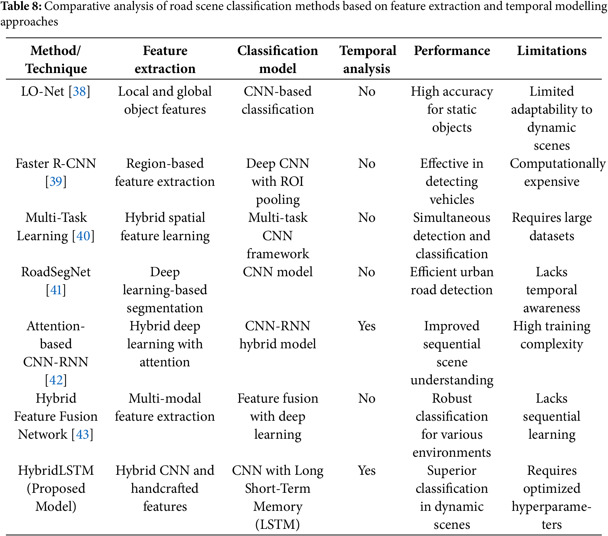
The HybridLSTM model effectively combines temporal learning with spatial convenience extraction, overcomes the drawbacks of earlier methods, and increases the classification accuracy of road scenes in dynamic environments, as demonstrated by this comparative research. It becomes gradually dependent, setting it apart from previous approaches and making it more appropriate for real-world autonomous driving applications.

4.1.1 Why HybridLSTM Outperforms Other Methods

HybridLSTM surpasses existing road scenes classification methods, integrating hybrid resource extraction, temporal modelling and computational efficiency. Unlike models such as faster R-CNN and LO-NET, which depend only on registration-based resource extraction, HybridLSTM combines CNN-based descriptors (Yolov5, VGG19) and handcrafted descriptors to capture high-level contextual and fine features. This hybrid approach enhances the model’s ability to distinguish visually similar road scenes, such as pedestrian bands in tunnel versus highways, improving robustness for occlusions and lighting variations. In addition, most previous methods, such as roadsegnet and hybrid resource fusion networks, lack temporal analysis, making them less effective in dynamic environments. HybridLSTM exceeds this limitation by integrating short-term memory networks (LSTM), allowing sequential dependencies to capture and perform well in change traffic conditions such as moving vehicles and variable climate.

In addition to accuracy, HybridLSTM reaches a balance between computational efficiency and real-time performance. Compared to deep-depth deep learning models such as CNN-RNN based on attention, HybridLSTM optimizes resource selection to reduce unnecessary calculations, maintaining a high classification accuracy of 96.3%. In addition, its cross-mastery adaptability, trained in various data sets (BDD100K, Kitti, Places-365 and LabelMe), ensures generalization for various road environments without extensive adjustment. These advantages make HybridLSTM a highly effective and scalable solution for real-world autonomous steering applications, addressing the limitations of existing methods and increasing accuracy, efficiency and adaptability in complex road scenes.

4.1.2 Unique Features of HybridLSTM

•   Hybrid Feature Extraction: Combines deep learning-based object detection (YOLOv5, VGG19) with handcrafted descriptors for comprehensive scene understanding.

•   Temporal Modelling with LSTM: Captures sequential dependencies, improving classification in dynamic and changing road environments.

•   Computational Efficiency: Optimized feature selection reduces processing overhead compared to other deep learning models.

•   High Classification Accuracy: Achieves 96.3% accuracy, 95.8% precision, 96.1% recall, and 96.0% F1-score, outperforming other methods.

•   Cross-Domain Generalization: Trained on multiple datasets (BDD100K, KITTI, Places-365, LabelMe), ensuring robustness across diverse road environments.

•   Real-World Applicability: Suitable for autonomous driving systems with minimal need for extensive dataset fine-tuning.

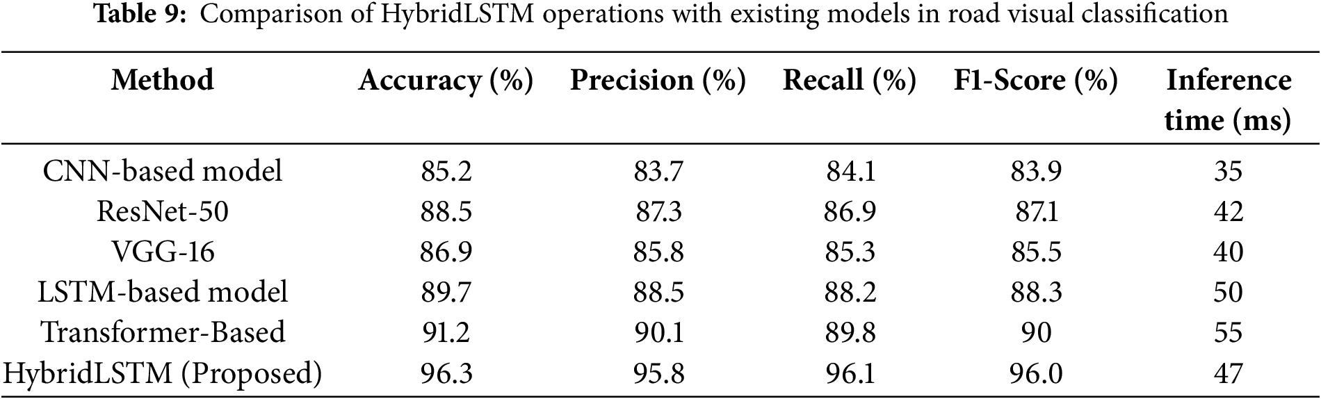
Table 9 shows how well the HybridLSTM model suggested compared to the most advanced methods currently used for road visual classification. Steps including processing time, F1-score, recall, accuracy, and accuracy are used to evaluate the influence of each model. The accuracy of Superior F1-Score and Classification shows how strong HybridLSTM is learning complex visual representations. HybridLSTM delivers better accuracy and recall than both standard LSTM and traditional CNN-based technologies, which reduces incorrect taxonomy rate. Moreover, when transformer-based models provide competitive accuracy, our method is more effective for real-time applications because it is much more calculative complexity and processing time than HybridLSTM. The effectiveness of HybridLSTM has been confirmed by this comparative study of HybridLSTM in getting the right trade between accuracy and calculative efficiency.

4.1.3 Mitigating High Computational Costs for Real-World Applications

HybridLSTM integrates object detection, deep learning-based scene feature extraction, and handcrafted feature analysis, making it computationally intensive. To mitigate this, several optimization strategies can be implemented:

•   Model Pruning and Quantization: Reducing the precision of weights (e.g., using INT8 instead of FP32) can significantly lower memory usage and computation costs without substantial accuracy loss.

•   Knowledge Distillation: Training a smaller, lightweight student model using the knowledge from the larger HybridLSTM model can retain classification performance while reducing computational overhead.

•   Efficient Feature Fusion: Instead of fusing high-dimensional feature vectors directly, dimensionality reduction techniques (e.g., PCA or autoencoders) can be applied to streamline processing.

•   Optimized Data Augmentation: Rather than performing complex augmentations at runtime, pre-processed and augmented datasets can be stored for efficient retrieval, reducing overhead.

•   Lightweight Backbone Models: Replacing VGG19 with a more computationally efficient CNN backbone (such as MobileNetV3 or Efficient Net) can reduce processing time while maintaining accuracy.

By incorporating these strategies, HybridLSTM can be optimized for real-world deployment on embedded systems while maintaining its superior classification accuracy and robustness in diverse road scenes.

5  Performance on Real-Time Road Scene Frames

Although datasets were produced for this work by collecting samples from various benchmark datasets and real-world scenarios, they were converted using videos captured in different geographical locations worldwide. Additionally, real-time videos of traffic scenes were obtained from various locations in Nagpur, Maharashtra, India. The acquisition device used was a Xiaomi Redmi Note 13 5G mobile phone, with 256 GB, 12 GB RAM, and 108 MP resolution with 30 frames per second. The mobile phone was mounted on one of the side mirrors of the car. The videos were captured during moderate and heavy traffic, and daytime and night. During the day, the weather was clear without any possibility of clouds or rain. The videos at night were captured when there was high illumination due to streetlights and lights from vehicles. A total of 17 such real traffic videos were captured with audio for a duration between 40–45 s. Therefore, the number of frames contained in a single video was approximately not below 1200.

The videos were converted to frames at a lower rate but not fixed. However, the frame rate was not below 10. The colour frames belonging to four classes were manually identified and sorted. Below are some sample images extracted from the videos. Figs. 15 and 16 show crosswalks at night and daytime. Figs. 17 and 18 show a highway scene from Nagpur to Wardha, Maharashtra, India.

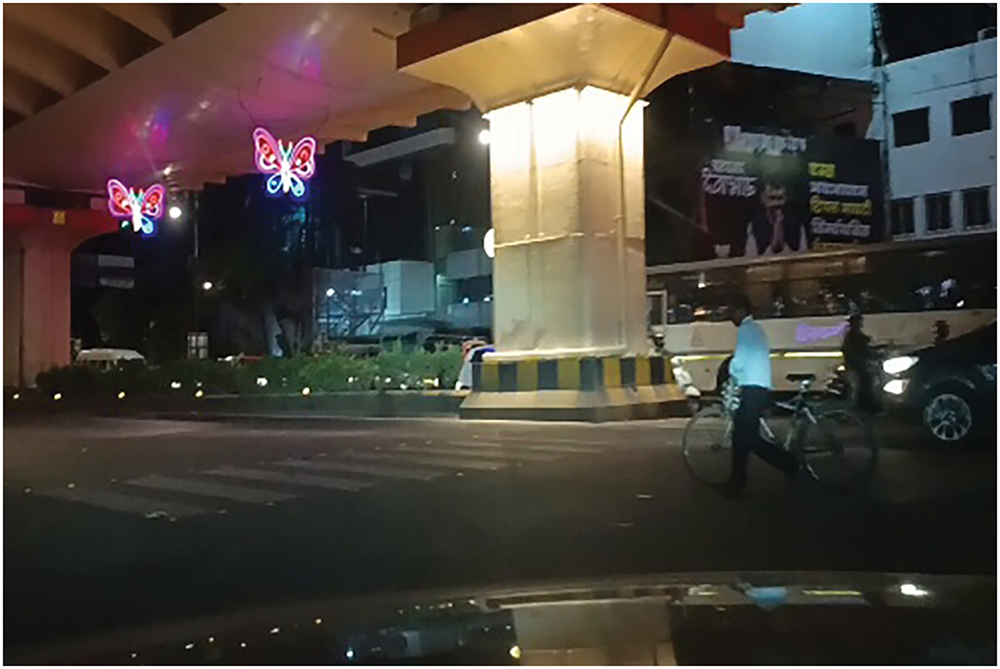
Figure 15: A real-time road traffic image depicting a crosswalk under a bridge at night

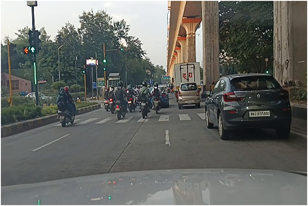
Figure 16: A real-time image depicting a crosswalk at daytime

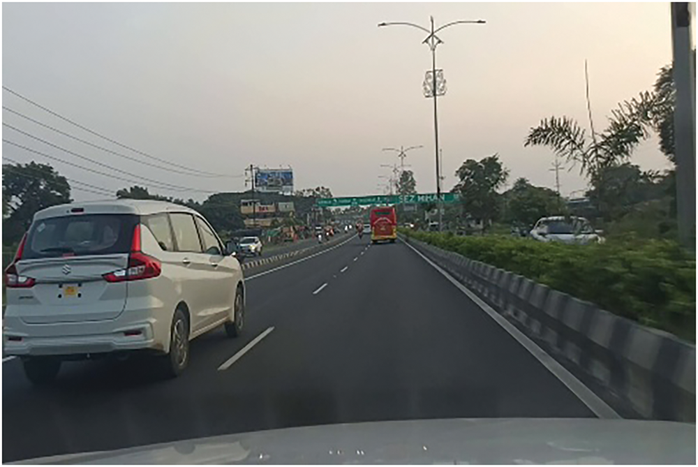
Figure 17: A real-time image depicting vehicles on a highway at daytime

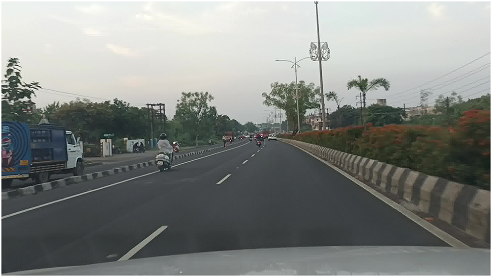
Figure 18: A real-time image depicting a highway at daytime

Figs. 19 and 20 depict the road under the metro bridge and tunnel road respectively from the Nagpur Chhatrapati Shivaji Maharaj Square and Manish Nagar underpass. The last sample image shown in Fig. 21 belongs to the roadside parking but is not allotted. That is the parking strips are missing but vehicles are allowed to be parked.

Figure 19: A real-time image depicting a road under a bridge at night

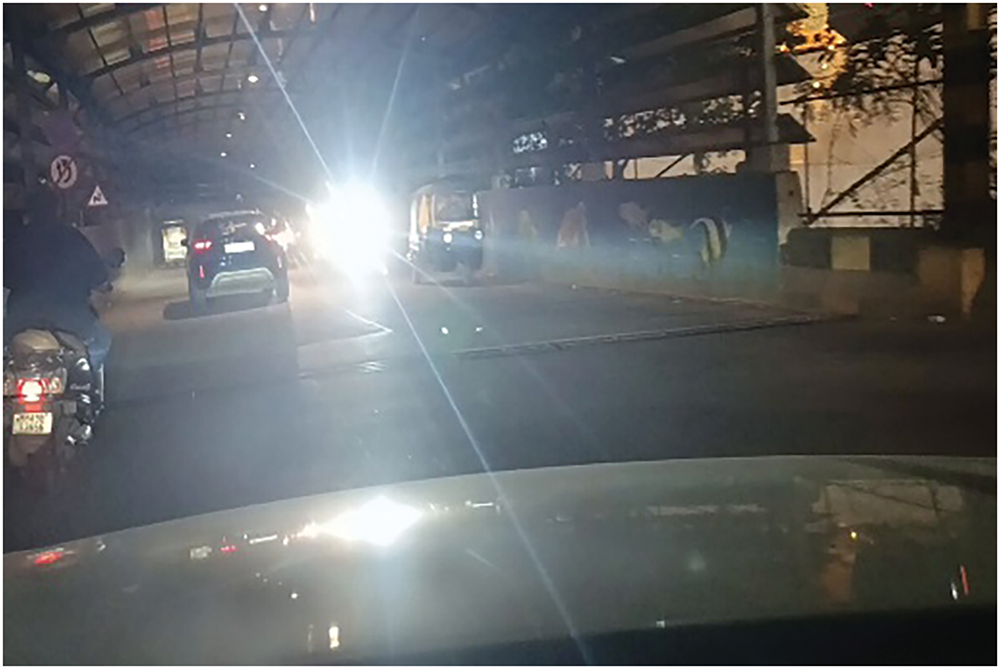
Figure 20: A real-time image depicting a tunnel road at night with high illumination

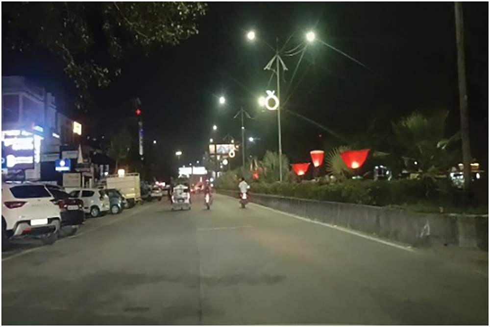
Figure 21: A real-time image depicting roadside parking (ambiguous) at night

The missing parking strips, the dimmed crosswalk, the crosswalk-under-bridge multiclass scenario, and the high illumination are intended to improve the challenges in the road scene images. The count of samples belonging to each of the categories is listed in Table 10. The maximum samples considered is 59 for the highway class and the minimum of 10 for the parking lot (ambiguous).

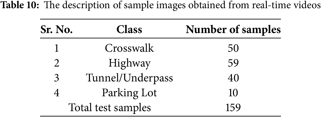
To analyze the scene classification network’s generalization ability, all previously collected samples from the benchmark dataset were used to train the classifier. No modifications were made to the classifier architectures or hyperparameters. Hybrid features were extracted from all 159 real-time acquired road scene images from videos, normalized using the Max-Normalization algorithm, with the mean considered over two samples for evaluation.

For Max-Normalization, the training set (2725 samples from four categories) and the testing set (159 samples) were concatenated to compute the maximum value of individual features. The samples were separated and subjected to compute the mean considering two adjacent feature values to alleviate the size of the feature vector. The performance of the classifier is shown in Table 9. It is observed that the customized LSTM network on real-time road scene frames outperforms the other two competing techniques.

6  Conclusion

The HybridLSTM framework introduced in this study offers a novel approach to road scene classification by effectively integrating deep learning-based, object-based, and handcrafted feature extraction techniques. This comprehensive fusion enables the model to capture both high-level contextual information and fine-grained details, leading to superior performance. Specifically, the model achieved a classification accuracy of 96.3%, precision of 95.8%, recall of 96.1%, and an F1-score of 96.0%, demonstrating its robustness across diverse road scenarios, including roadside parking, parking under tunnels, dimly lit crosswalks, and dynamic traffic conditions. Notably, HybridLSTM maintains high classification accuracy while minimizing computational complexity, making it well-suited for real-time road scene analysis.

However, opportunities for enhancement remain, particularly in addressing underrepresented classes such as overpass tunnels (OP/T) and improving the detection of specific elements like crosswalks through transfer learning. Future research directions will focus on improving the temporal modelling of sequential road scenes to enhance real-time decision-making in dynamic environments. Additionally, lightweight model adaptations for deployment on edge devices will be explored to reduce computational costs without compromising accuracy. Another avenue for improvement includes self-supervised and few-shot learning techniques to enhance classification performance with limited labelled data. Furthermore, extending HybridLSTM to multi-modal sensor fusion, incorporating LiDAR and radar data, could further improve robustness in low-visibility conditions. Addressing these challenges will contribute to the development of more efficient and reliable autonomous perception systems, strengthening the real-world applicability of HybridLSTM in intelligent transportation.

Acknowledgement: The authors would like to express their sincere gratitude to the G H Raisoni University, Amravati, a Research Center, for providing the necessary resources, infrastructure and continuous support throughout this research work. The guidelines and facilities extended by the university were fundamental in the successful conclusion of this study.

Funding Statement: The authors received no specific funding for this study.

Author Contributions: Sanjay P. Pande: authoring the first draft, taking the lead in method, inquiry, validation (equal), software (equal); Sarika Khandelwal: leading validation, leading supervision, editing the initial draft (equal), assisting with project management, supervising (equal), validation (equal); Ganesh K. Yenurkar: method (equal), formal analysis (equal), original draft editing (equal), validation (equal); Rakhi D. Wajgi: formal analysis (equal); Vincent O. Nyangaresi: comparable approach, formal analysis (equal); Pratik R. Hajare: resources; Poonam T. Agarkar: resources. All authors reviewed the results and approved the final version of the manuscript.

Availability of Data and Materials: No datasets were generated or analysed during the current study. The data was obtained from four benchmark datasets publicly available including Places-365 (https://paperswithcode.com/dataset/places365 (accessed on 01 January 2025)), BDD100K (https://www.kaggle.com/datasets/solesensei/solesensei_bdd100k, accessed on 01 January 2025), LabelMe (https://www.kaggle.com/datasets/dschettler8845/labelme-12-50k, accessed on 01 January 2025), and KITTI (https://www.kaggle.com/datasets/klemenko/kitti-dataset, accessed on 01 January 2025).

Ethics Approval: Not applicable.

Conflicts of Interest: The authors declare no conflicts of interest to report regarding the present study.

References

1. Everingham M, Van Gool L, Williams CK, Winn J, Zisserman A. The pascal visual object classes (voc) challenge. Int J Comput Vis. 2010;88(2):303–38. doi:10.1007/s11263-009-0275-4. [Google Scholar] [CrossRef]

2. Russakovsky O, Deng J, Su H, Krause J, Satheesh S, Ma S, et al. ImageNet large scale visual recognition challenge. Int J Comput Vis. 2015;115(3):211–52. doi:10.1007/s11263-015-0816-y. [Google Scholar] [CrossRef]

3. Deng J, Dong W, Socher R, Li LJ, Kai L, Li FF. ImageNet: a large-scale hierarchical image database. In: 2009 IEEE Conference on Computer Vision and Pattern Recognition; 2009 Jun 20–25; Miami, FL, USA. p. 248–55. doi:10.1109/CVPR.2009.5206848. [Google Scholar] [CrossRef]

4. Zhou B, Lapedriza A, Xiao J, Torralba A, Oliva A. Learning deep features for scene recognition using places database. Adv Neural Inf Process Syst. 2014;27:487–95. [Google Scholar]

5. Wang F, Ni W, Liu S, Xu Z, Wan Z. An intelligent pedestrian tracking algorithm based on sparse models in urban road scene. IEEE Trans Intell Transp Syst. 2024;25(3):3064–73. doi:10.1109/TITS.2023.3335654. [Google Scholar] [CrossRef]

6. Rangel JC, Cazorla M, García-Varea I, Martínez-Gómez J, Fromont É., Sebban M. Scene classification based on semantic labeling. Adv Robot. 2016;30(11–12):758–69. doi:10.1080/01691864.2016.1164621. [Google Scholar] [CrossRef]

7. Kostavelis I, Gasteratos A. Semantic mapping for mobile robotics tasks: a survey. Robot Auton Syst. 2015;66(01):86–103. doi:10.1016/j.robot.2014.12.006. [Google Scholar] [CrossRef]

8. Sitaula C, Xiang Y, Aryal S, Lu X. Scene image representation by foreground, background and hybrid features. arXiv:2006.03199. 2020. [Google Scholar]

9. Sikirić I, Brkić K, Bevandić P, Krešo I, Krapac J, Šegvić S. Traffic scene classification on a representation budget. IEEE Trans Intell Transp Syst. 2020;21(1):336–45. doi:10.1109/TITS.2019.2891995. [Google Scholar] [CrossRef]

10. Geiger A, Lenz P, Stiller C, Urtasun R. Vision meets robotics: the KITTI dataset. Int J Robot Res. 2013;32(11):1231–7. doi:10.1177/0278364913491297. [Google Scholar] [CrossRef]

11. Xue JR, Fang JW, Zhang P. A survey of scene understanding by event reasoning in autonomous driving. Int J Autom Comput. 2018;15(3):249–66. doi:10.1007/s11633-018-1126-y. [Google Scholar] [CrossRef]

12. Yang Y, Chen F, Wu F, Zeng D, Ji YM, Jing XY. Multi-view semantic learning network for point cloud based 3D object detection. Neurocomputing. 2020;397(11):477–85. doi:10.1016/j.neucom.2019.10.116. [Google Scholar] [CrossRef]

13. Xu H, Srivastava G. Automatic recognition algorithm of traffic signs based on convolution neural network. Multimed Tools Appl. 2020;79(17):11551–65. doi:10.1007/s11042-019-08239-z. [Google Scholar] [CrossRef]

14. Perumal PS, Sujasree M, Chavhan S, Gupta D, Mukthineni V, Shimgekar SR, et al. An insight into crash avoidance and overtaking advice systems for autonomous vehicles: a review, challenges and solutions. Eng Appl Artif Intell. 2021;104(1):104406. doi:10.1016/j.engappai.2021.104406. [Google Scholar] [CrossRef]

15. Bachute MR, Subhedar JM. Autonomous driving architectures: insights of machine learning and deep learning algorithms. Mach Learn Appl. 2021;6(8):100164. doi:10.1016/j.mlwa.2021.100164. [Google Scholar] [CrossRef]

16. Al-refai G, Al-refai M. Road object detection using Yolov3 and kitti dataset. Int J Adv Comput Sci Appl. 2020;11(8):48–54. doi:10.14569/ijacsa.2020.0110807. [Google Scholar] [CrossRef]

17. Qaddoura R, Bani Younes M, Boukerche A. Predicting traffic characteristics of real road scenarios in Jordan and gulf region. In: Proceedings of the 17th ACM Symposium on QoS and Security for Wireless and Mobile Networks; 2021 Nov 22–26; Alicante, Spain. p. 115–21. doi:10.1145/3479242.3487329. [Google Scholar] [CrossRef]

18. Qaddoura R, Younes MB. Temporal prediction of traffic characteristics on real road scenarios in Amman. J Ambient Intell Humaniz Comput. 2023;14(7):9751–66. doi:10.1007/s12652-022-03708-0. [Google Scholar] [CrossRef]

19. Kajiwara S. Evaluation of driver status in autonomous vehicles: using thermal infrared imaging and other physiological measurements. Int J Veh Inf Commun Syst. 2019;4(3):232. doi:10.1504/ijvics.2019.102224. [Google Scholar] [CrossRef]

20. Shen C, Zhao X, Fan X, Lian X, Zhang F, Kreidieh AR, et al. Multi-receptive field graph convolutional neural networks for pedestrian detection. IET Intell Transp Syst. 2019;13(9):1319–28. doi:10.1049/iet-its.2018.5618. [Google Scholar] [CrossRef]

21. van de Sande K, Gevers T, Snoek C. Evaluating color descriptors for object and scene recognition. IEEE Trans Pattern Anal Mach Intell. 2010;32(9):1582–96. doi:10.1109/TPAMI.2009.154. [Google Scholar] [PubMed] [CrossRef]

22. Zhang J, Marszałek M, Lazebnik S, Schmid C. Local features and kernels for classification of texture and object categories: a comprehensive study. Int J Comput Vis. 2007;73(2):213–38. doi:10.1007/s11263-006-9794-4. [Google Scholar] [CrossRef]

23. Krapac J, Verbeek J, Jurie F. Modeling spatial layout with fisher vectors for image categorization. In: 2011 International Conference on Computer Vision; 2011 Nov 6–13; Barcelona, Spain. p. 1487–94. doi:10.1109/ICCV.2011.6126406. [Google Scholar] [CrossRef]

24. Sánchez J, Perronnin F, Mensink T, Verbeek J. Image classification with the fisher vector: theory and practice. Int J Comput Vis. 2013;105(3):222–45. doi:10.1007/s11263-013-0636-x. [Google Scholar] [CrossRef]

25. Krizhevsky A, Sutskever I, Hinton GE. ImageNet classification with deep convolutional neural networks. Adv Neural Inf Process Syst. 2012;25(6):1097–105. doi:10.1145/3065386. [Google Scholar] [CrossRef]

26. Tang P, Wang H, Kwong S. G-MS2F: GoogLeNet based multi-stage feature fusion of deep CNN for scene recognition. Neurocomputing. 2017;225(2):188–97. doi:10.1016/j.neucom.2016.11.023. [Google Scholar] [CrossRef]

27. Simonyan K, Zisserman A. Very deep convolutional networks for large-scale image recognition. arXiv:1409.1556. 2014. [Google Scholar]

28. He K, Zhang X, Ren S, Sun J. Deep residual learning for image recognition. In: Proceedings of the 2016 IEEE Conference on Computer Vision and Pattern Recognition (CVPR); 2016 Jun 27–30; Las Vegas, NV, USA. p. 770–8. doi:10.1109/CVPR.2016.90. [Google Scholar] [CrossRef]

29. Bosch A, Munoz X, Oliver A, Marti R. Object and scene classification: what does a supervised approach provide us?. In: 18th International Conference on Pattern Recognition (ICPR'06); 2006 Aug 20–24; Hong Kong, China. p. 773–7. doi:10.1109/ICPR.2006.874. [Google Scholar] [CrossRef]

30. Ess A, Mueller T, Grabner H, van Gool L. Segmentation-based urban traffic scene understanding. In: Proceedings of the British Machine Vision Conference; 2009 Sep 7–10; London, UK. doi:10.5244/c.23.84. [Google Scholar] [CrossRef]

31. Di S, Zhang H, Mei X, Prokhorov D, Ling H. A benchmark for cross-weather traffic scene understanding. In: 2016 IEEE 19th International Conference on Intelligent Transportation Systems (ITSC); 2016 Nov 1–4; Rio de Janeiro, Brazil. p. 2150–6. doi:10.1109/ITSC.2016.7795904. [Google Scholar] [CrossRef]

32. Di S, Zhang H, Li CG, Mei X, Prokhorov D, Ling H. Cross-domain traffic scene understanding: a dense correspondence-based transfer learning approach. IEEE Trans Intell Transp Syst. 2018;19(3):745–57. doi:10.1109/TITS.2017.2702012. [Google Scholar] [CrossRef]

33. Zou Q, Jiang H, Dai Q, Yue Y, Chen L, Wang Q. Robust lane detection from continuous driving scenes using deep neural networks. arXiv:1903.02193. 2019. [Google Scholar]

34. Wang L, Li S, Yang F, Jiang X, Chen Z, Miao K, et al. Terrain preview detection and classification in unstructured scenes based on vision and laser fusion with deep learning. IEEE Access. 2024;12(4):137746–59. doi:10.1109/access.2024.3438247. [Google Scholar] [CrossRef]

35. Zhou W, Lv S, Jiang Q, Yu L. Deep road scene understanding. IEEE Signal Process Lett. 2019;26(4):587–91. doi:10.1109/lsp.2019.2896793. [Google Scholar] [CrossRef]

36. Guo YH, Zhu JR, Yang CC, Yang B. An attention-ReXNet network for long tail road scene classification. In: 2023 IEEE 13th International Conference on CYBER Technology in Automation, Control, and Intelligent Systems (CYBER); 2023 Jul 11–14; Qinhuangdao, China. p. 1104–9. doi:10.1109/CYBER59472.2023.10256482. [Google Scholar] [CrossRef]

37. Prykhodchenko R, Skruch P. Efficient multi-task learning for road scene classification: scene, time, and weather predictions. In: IEEE 20th International Conference on Intelligent Computer Communication and Processing (ICCP); 2024 Oct 17–19; Cluj-Napoca, Romania. p. 1–7. doi:10.1109/ICCP63557.2024.10793042. [Google Scholar] [CrossRef]

38. Li Y, Wu J, Liu H, Ren J, Xu Z, Zhang J, et al. Classification of typical static objects in road scenes based on LO-net. Remote Sens. 2024;16(4):663. doi:10.3390/rs16040663. [Google Scholar] [CrossRef]

39. Doğan G, Ergen B. A new CNN-based semantic object segmentation for autonomous vehicles in urban traffic scenes. Int J Multimed Info Retr. 2024;13(1):11. doi:10.1007/s13735-023-00313-5. [Google Scholar] [CrossRef]

40. Chaudhuri A. Smart traffic management of vehicles using faster R-CNN based deep learning method. Sci Rep. 2024;14(1):10357. doi:10.1038/s41598-024-60596-4. [Google Scholar] [PubMed] [CrossRef]

41. Du J, Ma L, Li J, Qin N, Zelek J, Guan H, et al. RdmkNet & Toronto-RDMK: large-scale datasets for road marking classification and segmentation. IEEE Trans Intell Transport Syst. 2024;25(10):13467–82. doi:10.1109/tits.2024.3394481. [Google Scholar] [CrossRef]

42. Alqarqaz M, Bani Younes M, Qaddoura R. An object classification approach for autonomous vehicles using machine learning techniques. World Electr Veh J. 2023;14(2):41. doi:10.3390/wevj14020041. [Google Scholar] [CrossRef]

43. Khan SA, Lee HJ, Lim H. Enhancing object detection in self-driving cars using a hybrid approach. Electronics. 2023;12(13):2768. doi:10.3390/electronics12132768. [Google Scholar] [CrossRef]

44. Khan SD, Basalamah S. Multi-branch deep learning framework for land scene classification in satellite imagery. Remote Sens. 2023;15(13):3408. doi:10.3390/rs15133408. [Google Scholar] [CrossRef]

45. Ni J, Shen K, Chen Y, Cao W, Yang SX. An improved deep network-based scene classification method for self-driving cars. IEEE Trans Instrum Meas. 2022;71:5001614. doi:10.1109/tim.2022.3146923. [Google Scholar] [CrossRef]

46. Narlawar MD, Pete DJ. Occluded face recognition: contrast correction & edge preserving enhancement based optimum features on CelebA dataset. J Harbin Eng Univ. 2023;44(8):1192–204. [Google Scholar]

47. Pal K, Yadav P, Katal N. RoadSegNet: a deep learning framework for autonomous urban road detection. J Eng Appl Sci. 2022;69(1):110. doi:10.1186/s44147-022-00162-9. [Google Scholar] [CrossRef]

48. Narayanan A, Dwivedi I, Dariush B. Dynamic traffic scene classification with space-time coherence. In: 2019 International Conference on Robotics and Automation (ICRA); 2019 May 20–24; Montreal, QC, Canada. p. 5629–35. doi:10.1109/icra.2019.8794137. [Google Scholar] [CrossRef]

49. Chen PR, Hang HM, Chan SW, Lin JJ. DSNet: an efficient CNN for road scene segmentation. APSIPA Trans Signal Inf Process. 2020;9(1):e27. doi:10.1017/atsip.2020.25. [Google Scholar] [CrossRef]

50. Lyu Y, Bai L, Huang X. Road segmentation using CNN and distributed LSTM. In: 2019 IEEE International Symposium on Circuits and Systems (ISCAS); 2019 May 26–29; Sapporo, Japan. p. 1–5. doi:10.1109/iscas.2019.8702174. [Google Scholar] [CrossRef]

51. Guo J, Wang J, Wang H, Xiao B, He Z, Li L. Research on road scene understanding of autonomous vehicles based on multi-task learning. Sensors. 2023;23(13):6238. doi:10.3390/s23136238. [Google Scholar] [PubMed] [CrossRef]

52. Zhao H, Qi X, Jia J. Multi-scale context aggregation for road scene segmentation with deep learning. Neurocomputing. 2022. doi:10.1016/j.neucom.2022.04.015. [Google Scholar] [CrossRef]

53. Li Y, Wang H, Dang LM, Nguyen TN, Han D, Lee A, et al. A deep learning-based hybrid framework for object detection and recognition in autonomous driving. IEEE Access. 2020;8:194228–39. doi:10.1109/access.2020.3033289. [Google Scholar] [CrossRef]

54. Bulo RS, Porzi L, Kontschieder P. Real-time road scene understanding using deep convolutional networks. Pattern Recognit Lett. 2022. doi:10.1016/j.patrec.2022.03.012. [Google Scholar] [CrossRef]

55. Hu Y, Wong Y, Wei W, Du Y, Kankanhalli M, Geng W. A novel attention-based hybrid CNN-RNN architecture for sEMG-based gesture recognition. PLoS One. 2018;13(10):e0206049. doi:10.1371/journal.pone.0206049. [Google Scholar] [PubMed] [CrossRef]

56. Zhu F, Cui J, Zhu B, Li H, Liu Y. Semantic segmentation of urban street scene images based on improved U-Net network. Optoelectron Lett. 2023;19(3):179–85. doi:10.1007/s11801-023-2128-8. [Google Scholar] [CrossRef]

57. Zhang Y, Zhang L, Wang Y, Xu W. AGF-Net: adaptive global feature fusion network for road extraction from remote-sensing images. Complex Intell Syst. 2024;10(3):4311–28. doi:10.1007/s40747-024-01364-9. [Google Scholar] [CrossRef]

58. Dolatyabi P, Regan J, Khodayar M. Deep learning for traffic scene understanding: a review. IEEE Access. 2025;13(2):13187–237. doi:10.1109/access.2025.3529289. [Google Scholar] [CrossRef]

59. Wang Y, Li Z, Wang J, Yang L, Dong B, Zhang H, et al. MFF: a deep learning model for multi-modal image fusion based on multiple filters. IEEE Access. 2025;13(10):38076–90. doi:10.1109/access.2025.3540007. [Google Scholar] [CrossRef]

60. Fan R, Li J, Li J, Wang J, Long Z, Jia N, et al. A glance over the past decade: road scene parsing towards safe and comfortable autonomous driving. Auton Intell Syst. 2025;5(1):8. doi:10.1007/s43684-025-00096-y. [Google Scholar] [CrossRef]

61. Kaur J, Singh W. Tools, techniques, datasets and application areas for object detection in an image: a review. Multimed Tools Appl. 2022;81(27):38297–351. doi:10.1007/s11042-022-13153-y. [Google Scholar] [PubMed] [CrossRef]

62. Khekare G, Yenurkar G, Turukmane AV, Ameta GK, Sharma P, Phulre AK. Artificial intelligence algorithms for better decision-making. In: Multi-criteria decision-making and optimum design with machine learning. Boca Raton, FL, USA: CRC Press; 2024. p. 252–62. doi: 10.1201/9781032635170-19. [Google Scholar] [CrossRef]

63. Bishop CM, Nasrabadi NM. Pattern recognition and machine learning. New York, NY, USA: Springer; 2006. [Google Scholar]

64. Pande SP, Khandelwal S, Hajare PR, Agarkar PT, Singh RD, Patil PR. Classification of road scenes based on heterogeneous features and machine learning. Int J Electr Comput Eng Syst. 2025;16(3):231–42. doi:10.32985/ijeces.16.3.4. [Google Scholar] [CrossRef]

65. Zhou B, Lapedriza A, Khosla A, Oliva A, Torralba A. Places: a 10 million image database for scene recognition. IEEE Trans Pattern Anal Mach Intell. 2017;40(6):1452–64. doi:10.1109/TPAMI.2017.2723009. [Google Scholar] [PubMed] [CrossRef]

66. Yu F, Xian W, Chen Y, Liu F, Liao M, Madhavan V, et al. BDD100K: a diverse driving dataset for heterogeneous multitask learning. In: Proceedings of the IEEE/CVF Conference on Computer Vision and Pattern Recognition (CVPR); 2020 Jun 13–19; Seattle, WA, USA. p. 2636–45. doi:10.1109/CVPR42600.2020.00271. [Google Scholar] [CrossRef]

67. Russell BC, Torralba A, Murphy KP, Freeman WT. LabelMe: a database and web-based tool for image annotation. Int J Comput Vis. 2008;77(1-3):157–73. doi:10.1007/s11263-007-0090-8. [Google Scholar] [CrossRef]

68. Geiger A, Lenz P, Urtasun R. Are we ready for autonomous driving? The KITTI vision benchmark suite. In: Proceedings of the IEEE Conference on Computer Vision and Pattern Recognition (CVPR); 2012 Jun 16–21; Providence, RI, USA. p. 3354–61. doi:10.1109/CVPR.2012.6248074. [Google Scholar] [CrossRef]