Software Defect Prediction Based on Semantic Views of Metrics: Clustering Analysis and Model Performance Analysis

1  Introduction

Software defect prediction is a key technology for ensuring software quality and reliability. Its goal is to identify potential defects by analyzing the static or dynamic features of software code [1]. The input of defect prediction models typically consists of software metrics, which are various indicators used to quantify software products or the software development process. Software metrics come in many forms, and their meanings can range from simple ones, such as the total number of lines of code, to more complex ones, like the maximum cyclomatic complexity or the average cyclomatic complexity. The output of a defect prediction model is a prediction of whether a defect exists, with two possible labels: defective or non-defective. However, with the increasing complexity of software systems, the proliferation of software metrics poses two major challenges for defect prediction. First, high-dimensional and redundant metrics impede model training efficiency and prediction accuracy. Second, significant variations in metric distributions across projects degrade cross-project prediction performance. To tackle these issues, feature selection, clustering, and efficient metric representation learning have emerged as key research directions.

This study focuses on clustering the features of metrics through clustering analysis methods, exploring the semantic view information of each cluster of software metrics, and investigating the impact of different views on software defect prediction based on the semantic views of metrics. The method proposed in this paper takes multiple software projects into comprehensive consideration, which helps to solve the redundancy problem in the current diverse software metrics and further improves the effectiveness and efficiency of defect prediction models.

Specifically, we first evaluated the silhouette coefficient [2] of the data from multiple software projects used in this study and obtained the expected number of clusters using a voting strategy similar to ensemble learning. According to this value, we applied multiple clustering analysis methods to each software project and recorded the clustering results. We introduced the co-occurrence matrix, which is commonly used in tasks related to natural language processing and social network analysis. This matrix can comprehensively consider the results obtained from multiple clustering methods of multiple projects. Then we further transformed the matrix into a distance matrix and applied hierarchical clustering to the distance matrix to obtain the classification results of software metrics that take all factors into account. After that, we analyzed the semantic commonalities of the software metrics in each category and obtained two semantic views of metrics. Finally, we conducted defect prediction experiments under different view conditions and analyzed the experimental results.

In summary, the main contributions of this study are threefold: (1) We propose a novel method for effectively clustering software metrics and deriving two semantic metric views; (2) Experimental results demonstrate that the combined semantic views outperform individual views in enhancing defect prediction performance; (3) Our findings reveal that the view focusing on internal design attributes significantly promotes the effect of software defect prediction.

The remainder of this paper is organized as follows: Section 2 reviews related work; Section 3 provides an overview of the proposed methodology; Section 4 details the determination of the optimal number of clusters; Section 5 elaborates on the process of acquiring semantic views of metrics; Section 6 presents the experimental design and analysis of results; and Section 7 concludes the paper. The tabular results corresponding to Section 6 are provided in Appendix A.

2  Related Work

Defect prediction holds practical significance today, as Abdou and Darwish [3] demonstrates that it can reduce resource waste during the development process and effectively improve software quality. Assim et al. [4] investigated and utilized multiple machine learning methods, such as SVM and decision trees, for software defect prediction, summarizing the characteristics and limitations of these models. Rahim et al. [5] proposed a machine learning-based software defect prediction framework consisting of data preprocessing, feature selection, and the application of machine learning models, and evaluated the performance of the Naive Bayes classifier in software defect prediction tasks. Curebal and Dag [6] examined the performance of Hist Gradient Boosting and other classifiers under feature selection, highlighting the importance of parameter tuning and method choice. Prabha and Shivakumar [7] proposed a hybrid method that combines principal component analysis with classification methods, improving the classification accuracy of large-scale datasets. Matloob et al. [8] explored the application of various methods in software defect prediction from the perspective of ensemble learning, emphasizing the importance of feature selection and model optimization. In [9], the researchers employed three ensemble algorithms integrating multiple classifiers for defect prediction and analyzed the impact of data preprocessing on defect prediction performance. Arya and Malik [10] focused on software defect prediction for web applications, proposing an enhanced machine learning approach that integrates K-means clustering with neural networks to improve prediction performance. Zhang et al. [11] used spectral clustering to divide software modules into two clusters, then labeled each cluster, proving the effectiveness of connectivity-based unsupervised learning methods in software defect prediction tasks. Balogun et al. [12] studied the application and performance of clustering techniques in software defect prediction and found that using clustering techniques as part of the classification process is feasible and provides good prediction performance. Jian et al. [13] proposed a hybrid feature selection method combining hierarchical clustering and ranking, grouping features through cluster analysis and then selecting representative feature subsets for defect prediction. In terms of multi-view approaches, Zhou et al. [14] introduced local structure preservation and adaptive weight allocation strategies, which are clustering methods focusing on incomplete views. Kiyak et al. [15] introduced a multi-view learning method for software defect prediction, applying the multi-view K-nearest neighbors algorithm to the field of software engineering. This method first constructs base classifiers to learn from each view and then combines the classifiers to create a robust multi-view model, enhancing defect prediction capabilities. Additionally, Chen et al. [16] proposed a data-driven multi-view learning method to effectively utilize diverse datasets with varying granularities and dimensions, helping models learn data features and improve defect prediction performance. In the context of code semantics, there exists research work that employs deep learning methods to represent code semantics and perform prediction tasks. Wang et al. [17] proposed a Deep Belief Network (DBN) that can automatically learn semantic features from abstract syntax trees and code changes. Abdu et al. [18] developed a defect prediction model that integrates semantic information from Abstract Syntax Trees (ASTs), Control Flow Graphs (CFGs), and Data Dependency Graphs (DDGs). Abdu et al. [19] proposed a novel defect prediction model that combines traditional features with code semantic features to address the limitations of single-feature-based approaches. While these works explore deep learning for code semantics [17–19], our study focuses on interpretable metric-based semantic views using traditional machine learning, thus employing different methodological premises.

3  Four-Step Semantic View Construction

The process of obtaining the semantic views of metric elements in this paper mainly consists of four main steps: (1) The first step is to determine the target number of clusters; (2) The second step is to conduct clustering experiments on each project using multiple clustering methods; (3) The third step is to synthesize all the clustering results; (4) The fourth step is to perform hierarchical clustering based on the synthesized results, and summarize the software metrics in each category from a semantic perspective. Eventually, the semantic views of metrics are obtained. The overall framework diagram is shown in Fig. 1. The first step is described in Section 4 of the paper, while the remaining three steps are presented in Section 5.

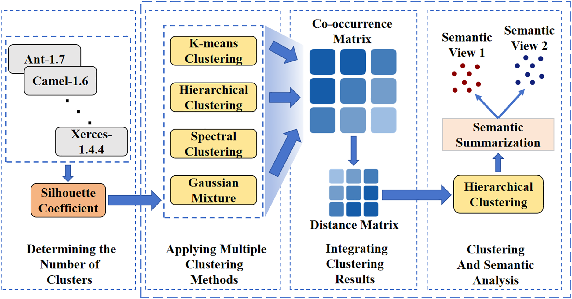
Figure 1: Semantic view construction framework for software metrics

Each procedural step is guided by the outcomes of its preceding step.

4  Determining the Number of Clusters

4.1 Dataset and Preprocessing

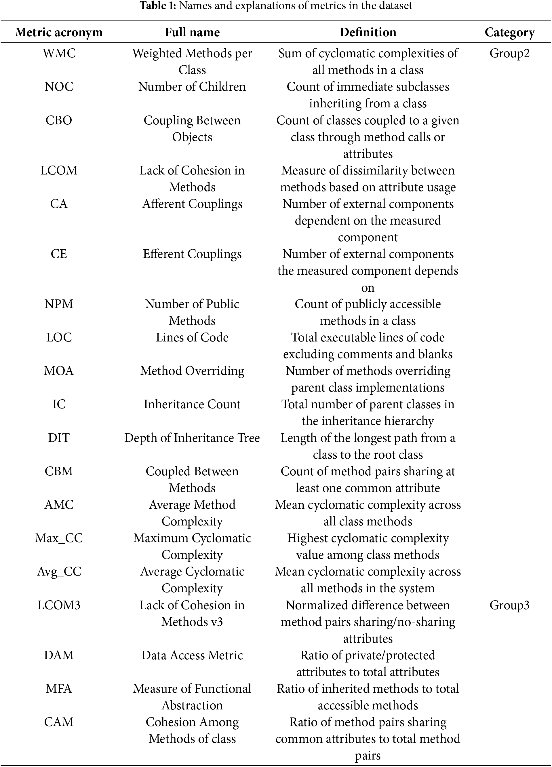
The PROMISE dataset [20], which contains open source Java projects, is utilized in this study. The projects in this dataset all contain the same set of software metrics. Each software metric has a distinct meaning, examining the quality of software code from different perspectives. Table 1 primarily introduces the abbreviations, full names, and corresponding meanings of the metrics in the dataset.

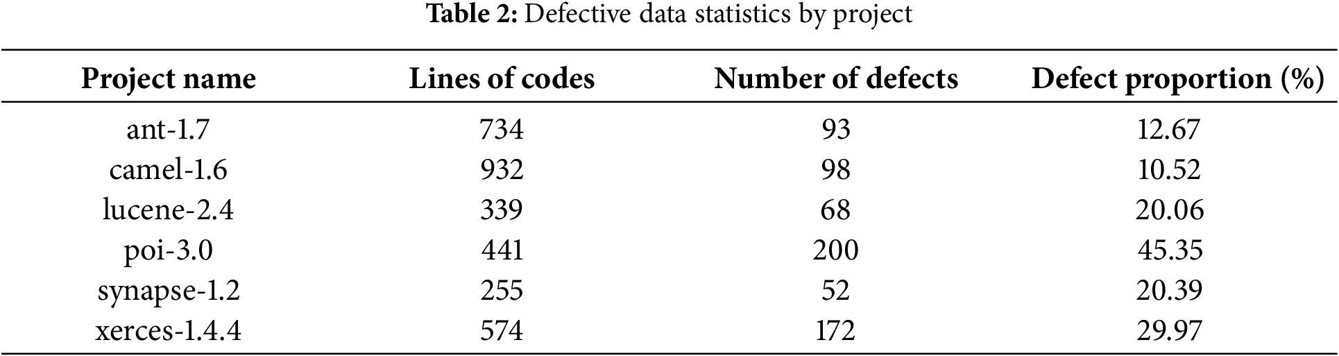
We selected six projects from the dataset: ant-1.7, camel-1.6, lucene-2.4, poi-3.0, synapse-1.2, and xerces-1.4.4. The number of data entries in each project ranges approximately from 250 to 950. The specific statistical results are shown in Table 2. Subsequently, we preprocessed the data by normalizing the metric data for each project. This step was taken to prevent the impact of different value ranges of the software metrics on the computational analysis, ensuring consistency and comparability in the data analysis.

4.2 Evaluation of the Silhouette Coefficient

s(i)=b(i)−a(i)max(a(i),b(i))(1)

To determine the optimal number of clusters, the silhouette coefficient was calculated for the data of each software project based on its values. The silhouette coefficient is an indicator used to evaluate the quality of clustering. Its core idea is to measure the compactness and separation of clustering results by computing the intra-cluster distance and inter-cluster distance for each sample. In Formula (1), a(i) represents the average distance from sample i to other samples in the same cluster, i.e., the intra-cluster distance, while b(i) represents the average distance from sample i to all samples in the nearest neighboring cluster, i.e., the inter-cluster distance.

The reasons for using this method are as follows: The silhouette coefficient takes into account both intra-cluster compactness and inter-cluster separation, providing a comprehensive reflection of the quality of clustering results. Compared to evaluation methods that rely solely on distance or density, the silhouette coefficient is more robust. Additionally, the silhouette coefficient is not dependent on a specific clustering algorithm and is applicable to various methods such as K-means, spectral clustering, Gaussian mixture clustering, and hierarchical clustering. Therefore, using the silhouette coefficient as a unified evaluation criterion ensures comparability across different methods. This method automatically selects the optimal number of clusters k by calculating the silhouette coefficient under different k values, choosing the k value that maximizes the silhouette coefficient. This avoids the subjectivity of manually setting k and ensures the scientific rigor of the experiment.

Moreover, compared to other evaluation methods such as the elbow method [21] and the Gap Statistic method, the silhouette coefficient has the following advantages: The elbow method relies more on subjective judgment and lacks a quantitative standard, while the Gap Statistic method has higher computational complexity and is more suitable for large-scale data.

Overall, the silhouette coefficient method is computationally simple, suitable for medium and small-scale data, and can quantify clustering effectiveness. In the task of software defect prediction, the silhouette coefficient can effectively identify cluster structures in metric data, helping to select the optimal k value and laying the foundation for subsequent experiments. Fig. 2 shows the curves of the silhouette coefficient as k varies for the six projects.

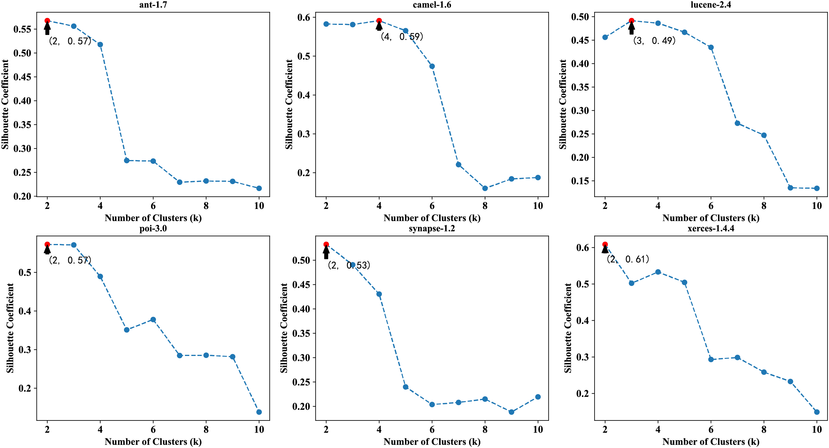
Figure 2: Silhouette coefficient vs. Number of clusters (k) for each project

The results in Fig. 2 indicate that, among the six projects, the optimal number of clusters is 2 for four projects, 3 for one project, and 4 for another project. Therefore, the predefined number of clusters was set to 2 for multiple clustering methods (K-means, spectral clustering, Gaussian mixture clustering, and hierarchical clustering), and further clustering experiments were conducted.

5  Acquisition of Semantic Views of Metrics

5.1 Applying Multiple Clustering Methods

The experiments utilized four methods: K-means, spectral clustering [22], Gaussian mixture clustering [23], and hierarchical clustering [24]. Overall, these methods analyze the clustering of software metrics from the perspectives of distance, graph theory, probability distribution, and hierarchical structure, respectively, aiming to obtain more comprehensive and robust clustering results. Specifically, the K-means method is based on the concept of distance, dividing the data into K clusters by calculating the distances between samples, ensuring that the distances within clusters are minimized while the distances between clusters are maximized. Spectral clustering is based on graph theory, treating data as nodes in a graph with similarity between nodes as edge weights, and performing dimensionality reduction and clustering using the eigenvalues and eigenvectors of the graph’s Laplacian matrix. Gaussian mixture clustering is based on a probabilistic model, assuming that the data is generated from a mixture of multiple Gaussian distributions, and determining the clustering results by estimating the parameters of each Gaussian distribution. Hierarchical clustering is based on hierarchical structure, constructing a hierarchical cluster tree by iteratively merging or splitting samples, which can be performed either bottom-up (agglomerative) or top-down (divisive).

Figs. A1 and A2 show Sankey diagrams of the clustering results for the six projects (ant, camel, etc.) under the four methods. The diagrams illustrate the specific distribution of metrics across different clusters for each project under various clustering methods. The results reveal that the six projects are not entirely consistent across the four clustering methods, necessitating further comprehensive analysis to weigh the clustering results of different methods (see Figs. A1 and A2 in Appendix A).

5.2 Integrating Clustering Results

Using the clustering results obtained by utilizing the four clustering methods to each project, a co-occurrence matrix was designed and constructed to quantify the frequency of different metrics appearing together in the same cluster. Specifically, the values in the co-occurrence matrix were initially set to 1. Subsequently, the clustering results of each project were iterated through using different methods. If two metrics appeared together in the same cluster, the corresponding value in the co-occurrence matrix was incremented by 1.

Fig. 3 presents a heatmap of the co-occurrence matrix, where the depth of color represents the frequency of co-occurrence between metrics, with darker shades indicating higher frequencies and lighter shades indicating lower frequencies.

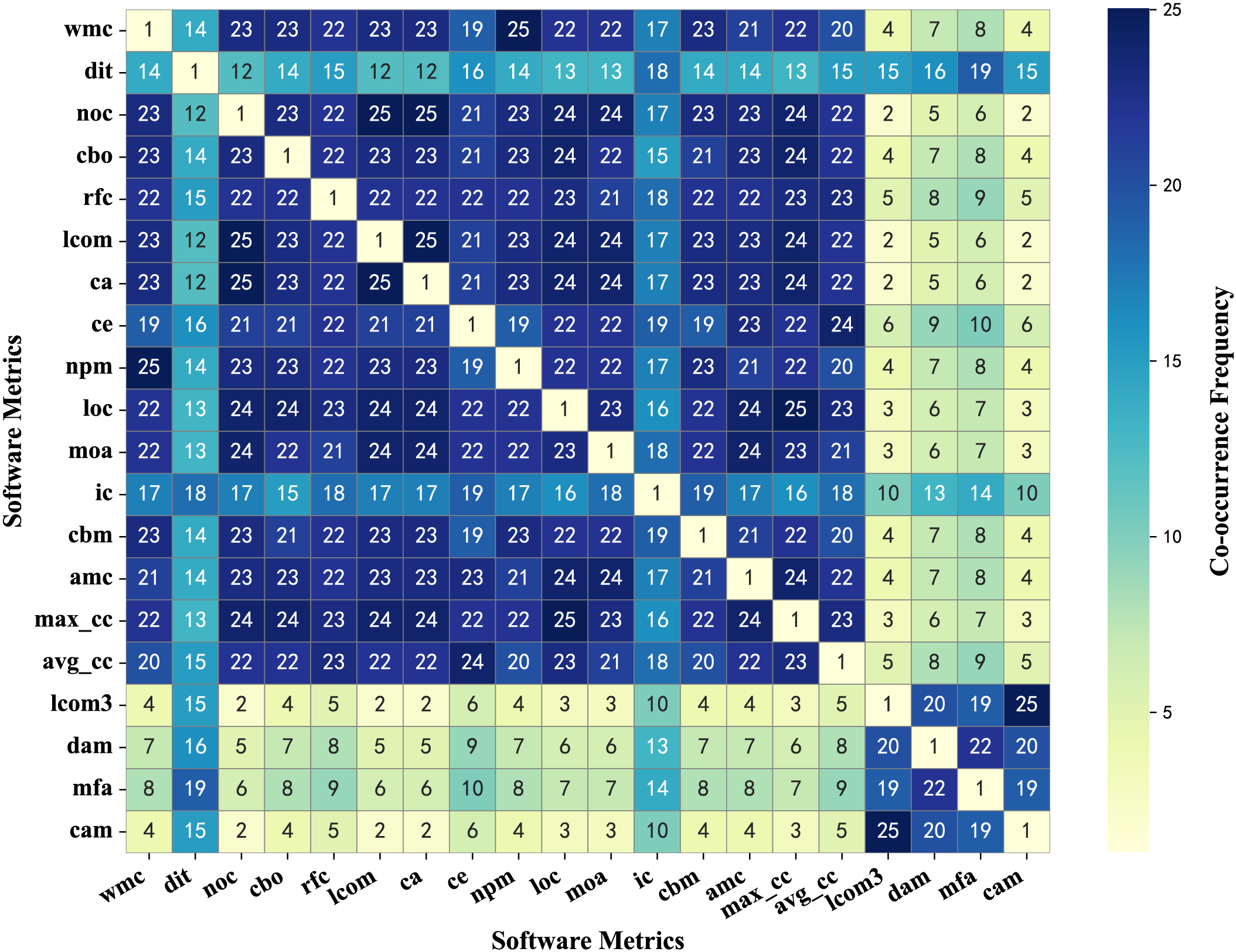
Figure 3: Heatmap of co-occurrence matrix for metrics

The co-occurrence matrix was transformed into a distance matrix embodying the concept of distance, with normalization applied to mitigate the influence of varying distance scales.

Subsequently, the normalized co-occurrence matrix was further converted into a distance matrix. This distance matrix represents the comprehensive results of multiple clustering methods across various projects, where a higher frequency of co-occurrence in the same cluster corresponds to a closer distance.

d_matrix=(1−n_matrix)⋅I(n_matrix≠0)(2)

In Formula (2), I(n_matrix≠0) is an indicator function, where n_matrix represents the elements of the matrix after normalization, and d_matrix represents the elements of the computed distance matrix. When the element value is not zero, the indicator function value is 1; when the element value is zero, the indicator function value is 0. Fig. 4 shows the distance matrix obtained after the above processing, where darker colors represent greater distances between the elements.

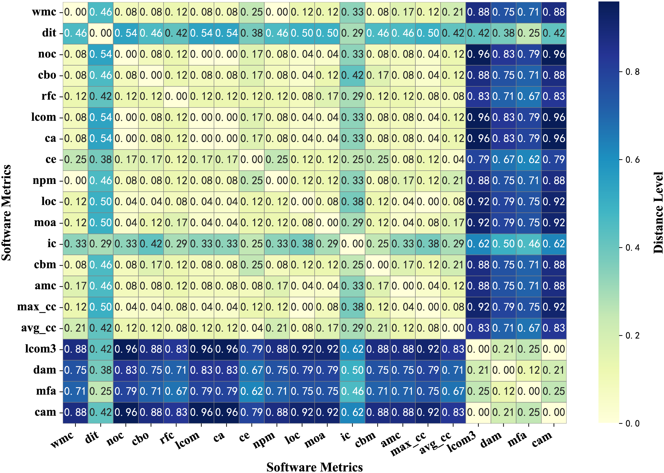
Figure 4: Heatmap of distance matrix for metrics

5.3 Clustering and Semantic Analysis

After compressing the distance matrix, a dynamic hierarchical clustering method, which does not require a pre-set number of clusters, was applied, and the clustering process was visualized. Fig. 5 shows the result of dynamic hierarchical clustering, indicating that two major clusters are clearly separated when the inter-cluster distance reaches around 0.4.

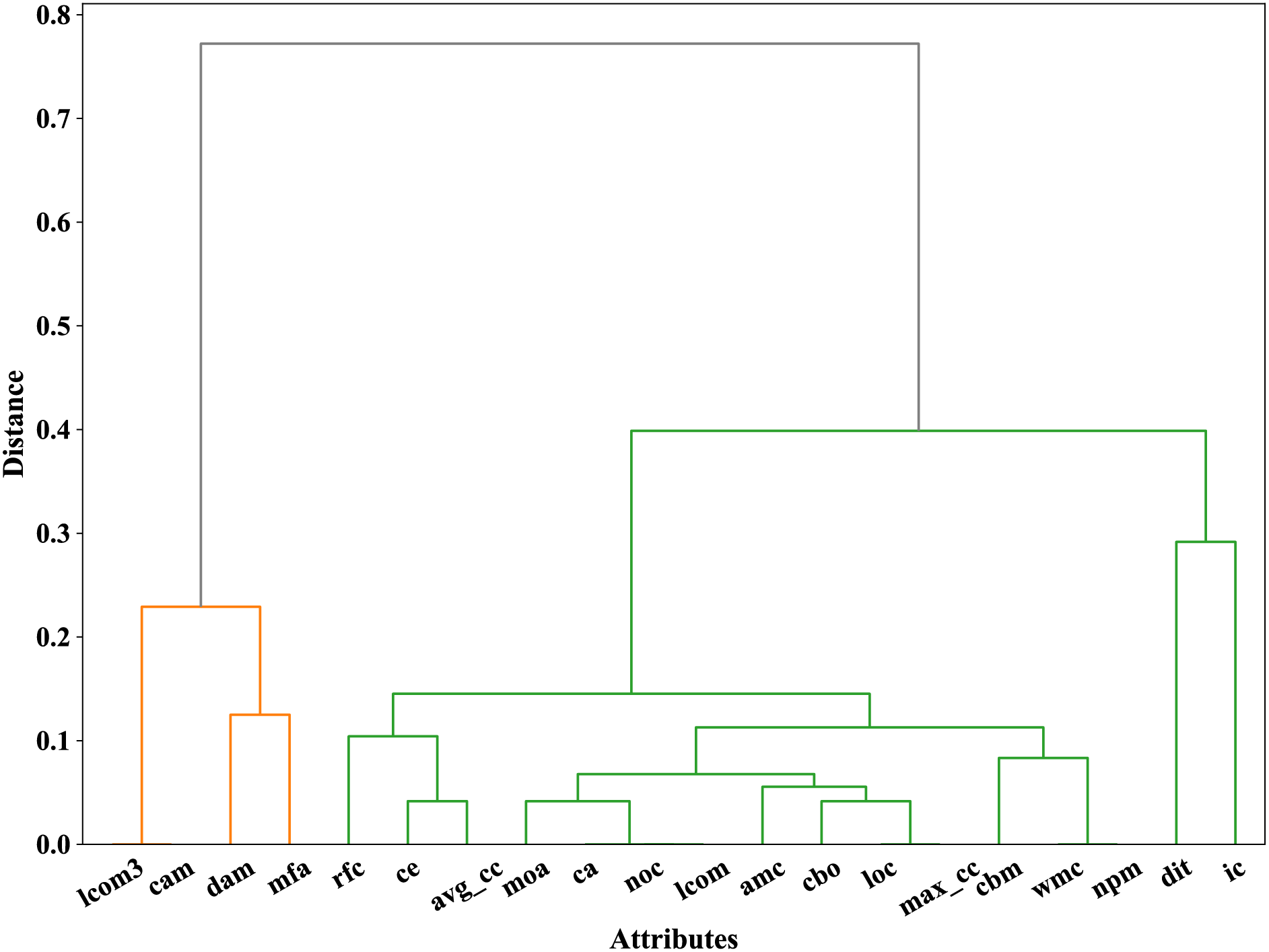
Figure 5: Dendrogram from dynamic hierarchical clustering

Since we selected a predefined cluster number of 2 based on the analysis of the optimal number of clusters for each project, and the visualization results of dynamic hierarchical clustering showed that two distinct clusters of metrics could be clearly identified at a distance of approximately 0.4, we obtained two groups of software metrics through the above analysis process. The grouping results are shown in Table 1. The first 16 mretrics belong to Group2, and the last 4 metrics belong to Group3.

In the two metric groups, the first group contains a larger number of metrics, including WMC, NOC, CBO, LCOM, CA, CE, NPM, LOC, MOA, IC, DIT, CBM, AMC, Max_CC, and Avg_CC. These metrics primarily focus on the scale, complexity, and interdependencies between modules of the software system, emphasizing the macro-level properties of the code. The second group contains fewer metrics, including LCOM3, DAM, MFA, and CAM, which focus on evaluating the design quality of classes and their internal structural characteristics, emphasizing the internal design of the software code.

Based on the above grouping results, we obtained two semantic views of metrics with different semantic characteristics. To further validate the effectiveness of single-view vs. multi-view approaches in defect prediction tasks, we conducted experiments using various classification methods for software defect prediction.

6  Defect Prediction Experiment

6.1 Preparation for the Experiment

Experiments were conducted based on semantic views of metrics using multiple classifiers to explore the different effects of various semantic views of metrics on software defect prediction tasks and the extent to which they influence the performance of different classification models. The classifiers utilized in this study are Support Vector Machine (SVM) [25], Random Forest [26], XGBoost [27], K-Nearest Neighbors (KNN) [28], Logistic Regression [29] and Hist Gradient Boosting.

Among these six classifiers, SVM distinguishes data of different classes by finding the maximum margin, making it suitable for high-dimensional spaces and scenarios where the number of samples is less than the number of features, with strong generalization capabilities. Random Forest is an ensemble learning method that improves model accuracy and stability by constructing multiple decision trees and combining their predictions, excelling in handling high-dimensional data and large datasets. XGBoost (Extreme Gradient Boosting) is a gradient boosting-based ensemble learning method that iteratively adds tree models to minimize the loss function, often delivering excellent performance across various datasets, particularly on structured data. KNN is an instance-based learning algorithm that predicts the class of a sample by voting based on the classes of its K nearest neighbors, suitable for small-scale and low-dimensional datasets but computationally intensive for large datasets. Logistic Regression is a log-odds model used for binary classification, predicting the probability of an event occurring, with a simple and interpretable model. Hist Gradient Boosting is a relatively novel histogram-based gradient boosting algorithm that discretizes continuous features into histograms, offering high computational efficiency. Each of the six classifiers has different emphases, enabling us to summarize and analyze the experimental results of each type of classifier.

In the software defect prediction experiment, three metric groups—Group1, Group2, and Group3—were designed: Group1 represents a comprehensive semantic view, encompassing all software metrics, while Group2 and Group3 are independent semantic views constructed based on the first and second metric groupings, respectively, focusing on the macro-level and internal aspects of the software code. By comparing the predictive performance of six classifiers across Group1, Group2, and Group3, we can gain a more comprehensive understanding of the impact of different metric groups on software defect prediction effectiveness.

In the software defect prediction experiments, data preprocessing is a critical step to ensure model performance. The experiment utilized a series of data processing methods, including oversampling, stratified sampling, and Principal Component Analysis (PCA) for dimensionality reduction.

As shown in Table 2, the software defect data suffers from class imbalance, where the number of defect samples is significantly lower than that of non-defect samples. Training models directly on raw data may result in overfitting to non-defect samples and inadequate recognition of defect samples. To effectively address this issue, the Synthetic Minority Oversampling Technique [30] (SMOTE) was utilized to oversample the minority class. SMOTE balances the dataset by synthesizing new samples for the minority class. For each minority class sample xi, SMOTE identifies its k nearest neighbors, randomly selects one neighbor xj, and generates a new sample xnew through linear interpolation, where λ is a random value determining the interpolation position, as shown in Formula (3):

xnew=xi+λ⋅(xj−xi)(3)

After applying this oversampling method, the number of defect and non-defect samples becomes balanced, thereby enhancing the model’s ability to recognize minority classes.

Additionally, to ensure that the training and test sets maintain a 1:1 ratio of non-defect to defect samples after oversampling, the experiment utilized stratified sampling to partition the dataset. The stratified sampling method divides the data into training and test sets based on the proportion of defect and non-defect samples in the overall dataset, ensuring consistency in the distribution of classes between the two sets. This means that the label proportions in the training and test sets are the same, thereby ensuring a more balanced training and testing process for the model.

The software metric data includes multiple metrics (such as WMC, CBO, LOC, etc.), which may suffer from redundancy, leading to inefficient model training and potential overfitting. To reduce feature dimensionality, eliminate redundant information, and extract key features, the experiment utilized Principal Component Analysis (PCA) for dimensionality reduction before training and testing the classifiers. PCA is a statistical method that transforms a set of correlated variables into a new set of linearly uncorrelated variables, known as principal components, through orthogonal transformation. This process aims to reduce the dimensionality of the data while retaining as much of the characteristic information of the original data as possible. It begins by calculating the covariance matrix C of the data:

C=1NXTX(4)

Among them, X is the original data matrix and N is the number of samples. Subsequently, eigenvalue decomposition is performed on the covariance matrix, and the eigenvectors corresponding to the top k largest eigenvalues are selected to form the projection matrix W. Then, the data is projected onto the low–dimensional matrix Z, completing the dimensionality reduction of the data. The core calculation process is as follows:

Z=XW(5)

In terms of performance measures, AUC (Area Under the Curve) and Accuracy were selected as the quantitative metrics, which can more comprehensively reflect the model’s overall classification ability and its capability to distinguish between the two classes under various threshold conditions [31]. This allows for a more comprehensive and objective assessment of the model’s performance. AUC, as the name suggests, is the area under the ROC (Receiver Operating Characteristic) curve and is used to evaluate the overall performance of a classification model at different threshold values. The ROC curve has the True Positive Rate (TPR) on the y-axis and the False Positive Rate (FPR) on the x-axis. The formulas for calculating TPR and FPR are as follows:

TPR=TPTP+FN(6)

FPR=FPFP+TN(7)

TP (True Positives) refers to the number of samples that are correctly predicted as the positive class by the model; FN (False Negatives) refers to the number of positive class samples that are incorrectly predicted as the negative class by the model; FP (False Positives) refers to the number of negative class samples that are incorrectly predicted as the positive class by the model; TN (True Negatives) refers to the number of samples that are correctly predicted as the negative class by the model. The formula for calculating AUC is the area under the ROC curve:

AUC=∫01TPR(FPR)d(FPR)(8)

Accuracy (Acc) is the proportion of correctly predicted samples by the classification model out of the total number of samples, and it is the most intuitive indicator for evaluating classification performance. It is formally defined as:

Accuracy=TP+TNTP+TN+FP+FN(9)

The reason for using both AUC and Acc is that AUC can comprehensively evaluate the model’s performance at different thresholds and can evenly reflect the model’s ability to distinguish between positive and negative samples. Accuracy, on the other hand, intuitively represents the model’s classification accuracy for the overall data. The combined use of the two can provide a more comprehensive understanding of the model’s overall performance and its ability to identify the minority class, avoiding the evaluation bias that may be caused by a single indicator and thus more accurately reflecting the model’s performance.

6.2 Results and Analysis

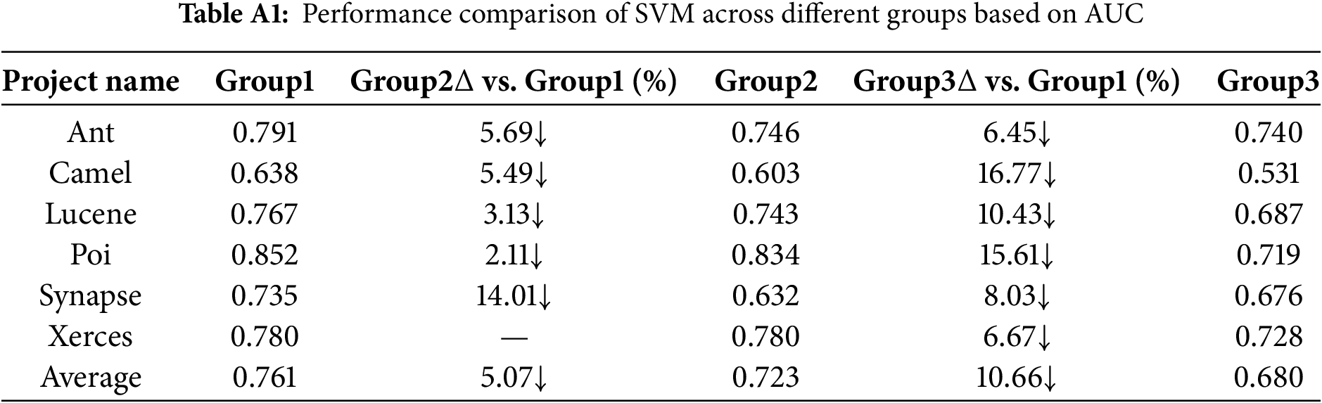
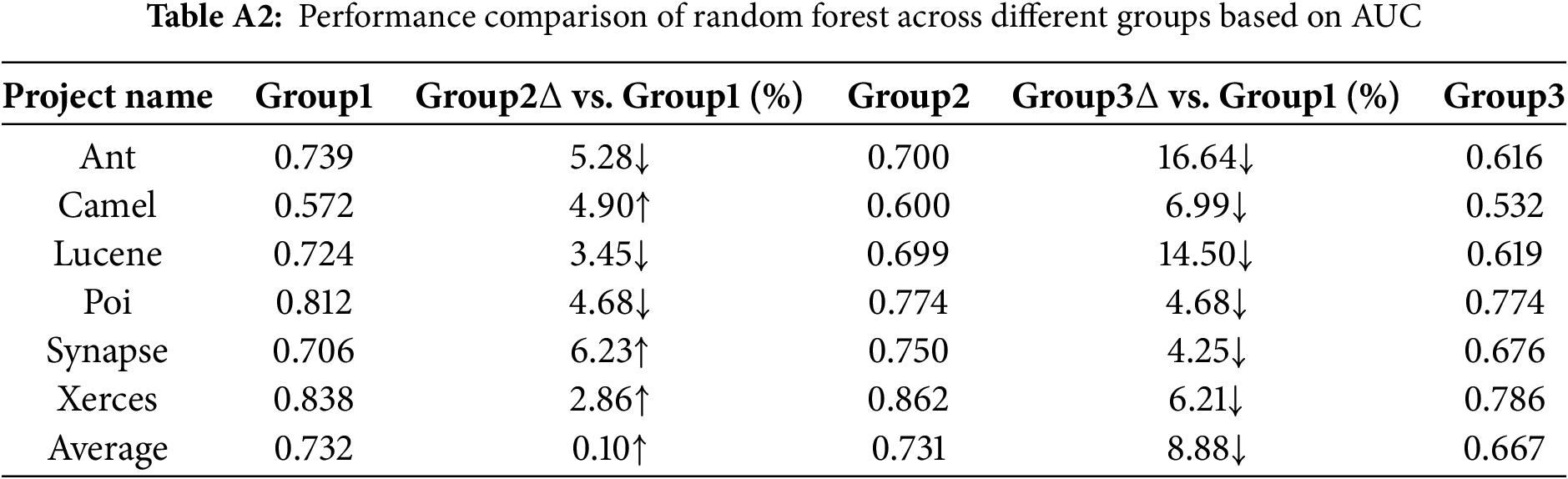
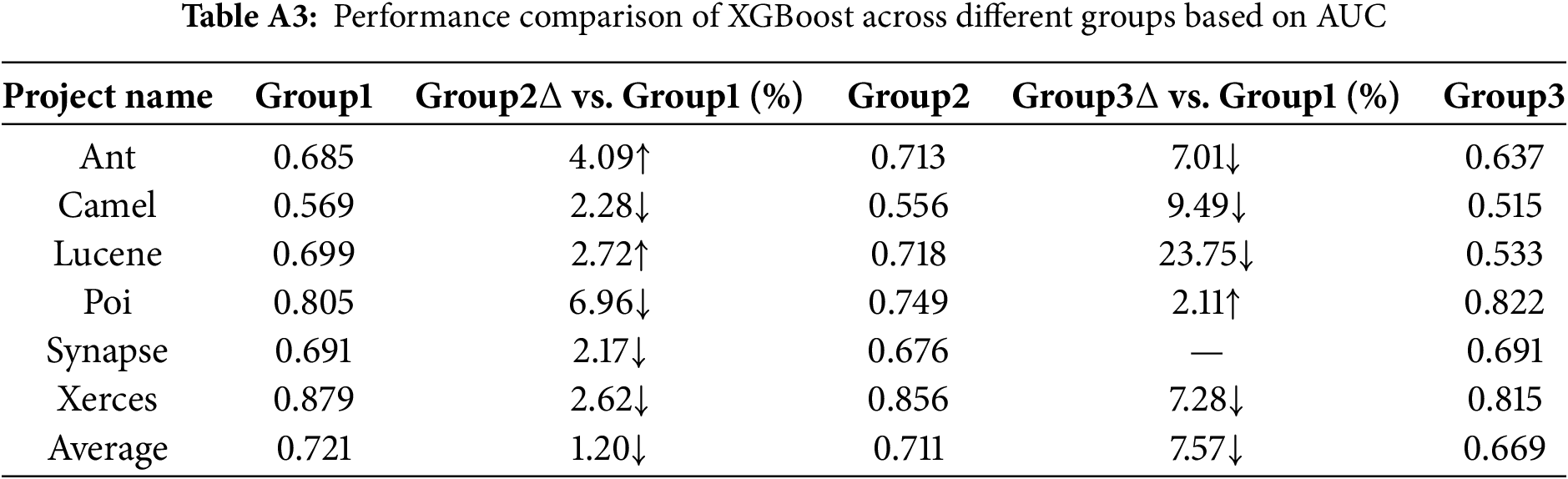
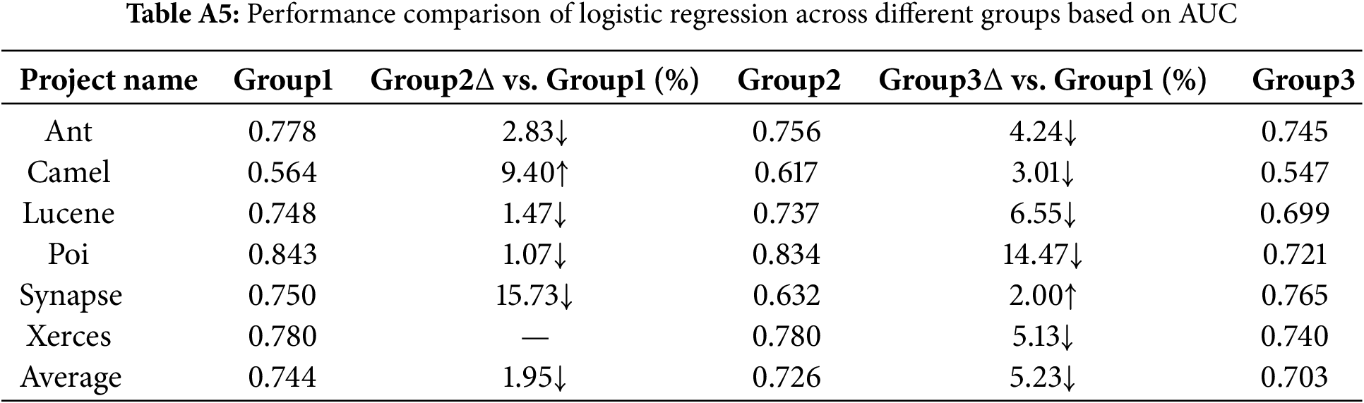
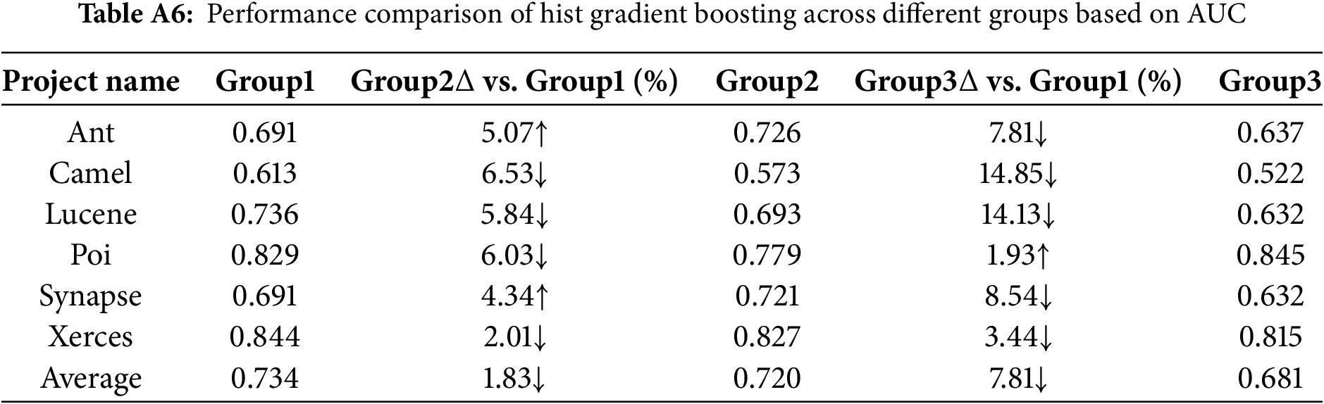
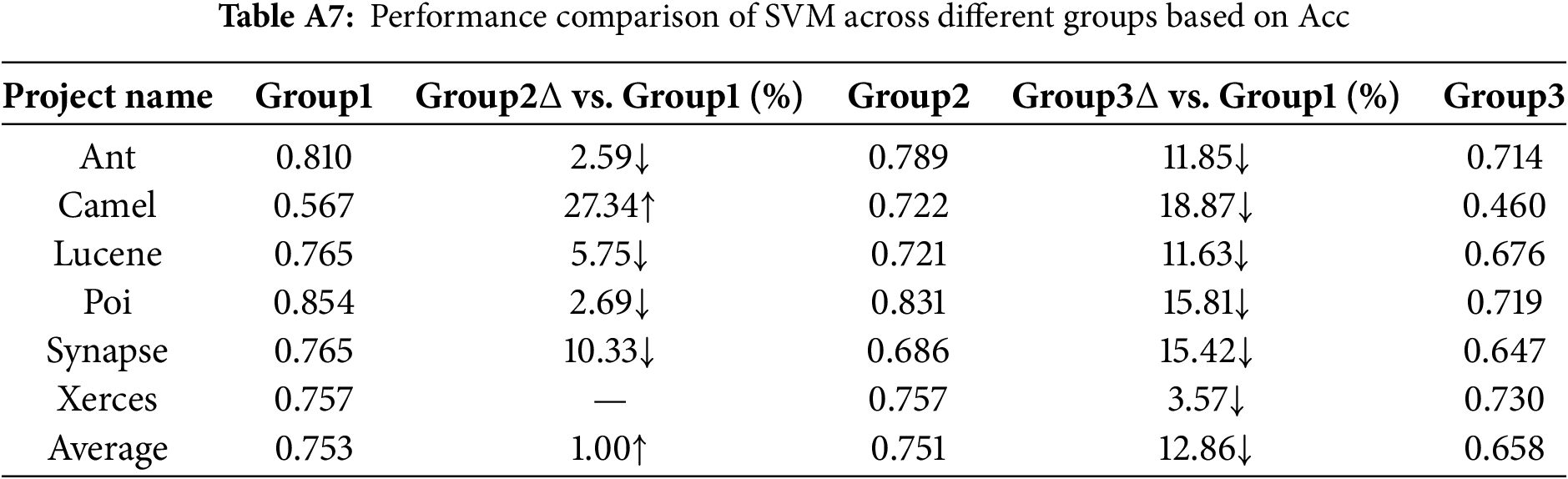
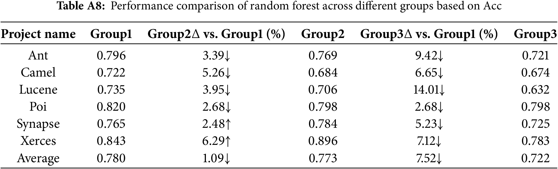
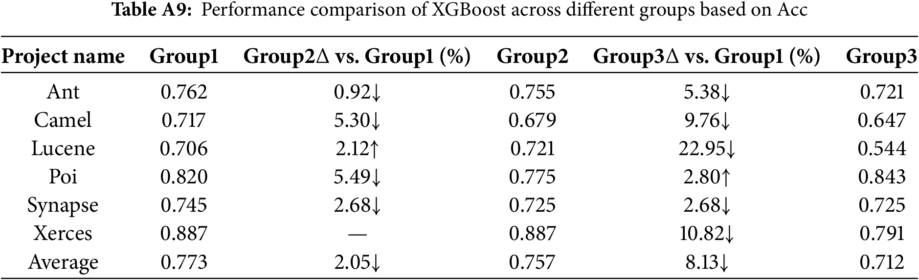
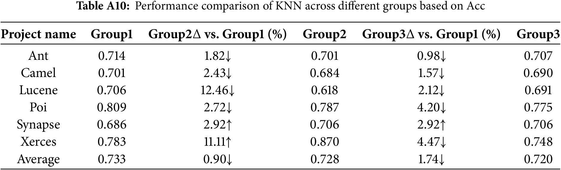
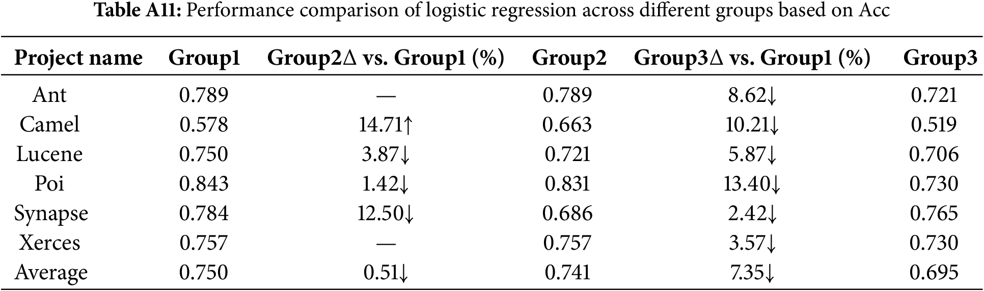
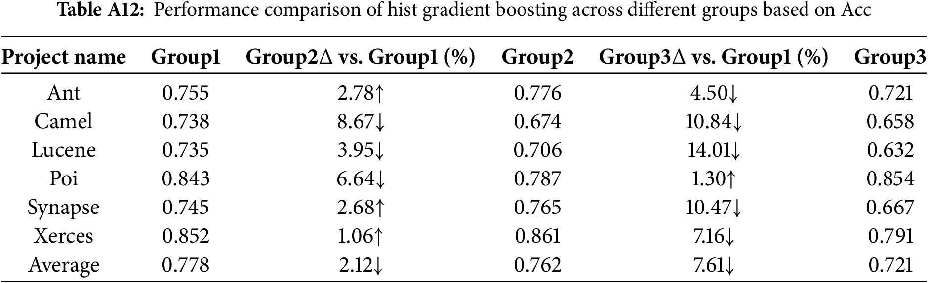
The multiple tables of experimental results are included in Appendix A. Tables A1 through A11 summarize the AUC and Acc values of the prediction results across different Group conditions, comparing the performance of six methods for each project. In the tables, Δ represents the amount of change, and — indicates no change.

6.2.1 Overall Performance of Different Classification Models

For the SVM model, under the Group1 condition, the performance in terms of AUC and Acc is generally better than that under Group2 and Group3. Specifically, for AUC, the average value under Group1 is 5.07% and 10.66% higher than that under Group2 and Group3, respectively, indicating a significant impact.

The Random Forest model shows relatively stable performance in terms of AUC. However, for Acc, the performance under Group1 is significantly better than that under Group2 and Group3. This suggests that Random Forest is somewhat sensitive to the increase in software metrics in terms of overall classification accuracy.

XGBoost demonstrated significant advantages in both AUC and Accuracy for the Group1 view, particularly when compared to Group3, with substantial improvements in AUC and Accuracy, indicating a higher sensitivity

KNN exhibits relatively stable performance in both AUC and Accuracy compared to other models, though the results under the Group1 view still demonstrate a certain level of advantage.

The Logistic Regression model shows a performance trend similar to the XGBoost model in terms of AUC and Acc, with a particularly noticeable improvement in AUC and Acc under Group1 compared to Group3.

The overall performance of Hist Gradient Boosting in terms of AUC and Acc is comparable to the experimental results of the XGBoost method.

6.2.2 The Impact of the Combination of Group2 and Group3 on Model Performance

Based on the results of AUC and Acc, for the majority of classification models in the experiment, the AUC and Acc under Group1 are generally higher than the single-view performance of Group2 and Group3. This indicates that combining Group2 and Group3 can enhance model performance in most cases. These findings suggest that the increased diversity of software metrics positively contributes to the improvement of model prediction performance. The inclusion of new semantic views of metrics provides additional semantic information, enabling models to better capture underlying patterns in the data.

6.2.3 The Contribution of Metrics in Group2 and Group3 to Model Performance

Group1 is equivalent to the integration of Group2’s software metrics into Group3, with Group2 containing a larger number of software metrics. The inclusion of Group2 demonstrates a significant positive effect across all models, substantially improving both AUC and Acc metrics.

Although Group3 contains only four software metrics, its incorporation demonstrates a significant impact on model performance. In the majority of cases, the inclusion of Group3 further enhances the predictive effectiveness under the Group2 condition; in fewer instances, its addition may slightly reduce the predictive performance under the Group2 condition. This indicates that despite the limited number of metrics in Group3, it encapsulates certain critical information, which overall contributes to a substantial improvement in model performance.

7  Conclusion

Software metric grouping: Through experiments, we obtained two semantic views of metrics, each focusing on the macro-level code characteristics and the internal design quality of software projects, respectively.

The effect of semantic view fusion: Compared to the Group2 and Group3 views, the Group1 condition significantly enhances model performance in terms of AUC and Acc in the majority of cases, demonstrating that the fusion of semantic views of software metrics plays a crucial role in improving model effectiveness.

Sensitivity of models to the increase in software metrics: From a performance perspective, SVM, XGBoost, Hist Gradient Boosting and Random Forest exhibit higher sensitivity. In contrast, Logistic Regression demonstrates relatively lower sensitivity.

The key role of Group3: Despite having fewer software metrics, the addition of Group3 significantly improves model performance in the majority of cases, indicating that these metrics contain certain key information.

Limitations: First, the experimental data primarily relies on software projects from the PROMISE dataset, and the diversity of the data could be further improved. Second, although scientific evaluation metrics and methods were adopted during clustering and semantic view partitioning, some subjectivity may still exist, potentially affecting the accuracy of clustering results and the validity of semantic views.

Future Work: Based on current limitations, future research could focus on: (1) Expanding the dataset to include more diverse software projects (in type, scale, and domain) to enhance result reliability; (2) Developing more objective and precise clustering methods and semantic view partitioning strategies to minimize subjective bias; (3) Investigating relationships between different semantic views to strengthen theoretical foundations and practical guidance for defect prediction.

Acknowledgement: The authors are grateful to the reviewers and editors for their valuable comments and suggestions.

Funding Statement: This study was supported by the CCF-NSFOCUS ‘Kunpeng’ Research Fund (CCF-NSFOCUS 2024012).

Author Contributions: The authors confirm their contribution to the paper as follows: conceptualization, methodology: Baishun Zhou, Haijiao Zhao; investigation: Yuxin Wen, Gangyi Ding, Xinyang Lin; experiment: Baishun Zhou, Haijiao Zhao; analysis: Baishun Zhou, Haijiao Zhao, Yuxin Wen, Lei Xiao; writing: Baishun Zhou, Haijiao Zhao, Yuxin Wen, Gangyi Ding, Ying Xing; supervision: Ying Xing. All authors reviewed the results and approved the final version of the manuscript.

Availability of Data and Materials: The data that support the findings of this study are openly available at https://github.com/feiwww/PROMISE-backup (accessed on 10 June 2025).

Ethics Approval: Not applicable.

Conflicts of Interest: The authors declare no conflicts of interest to report regarding the present study.

Appendix A Tables and Figures of Experimental Results

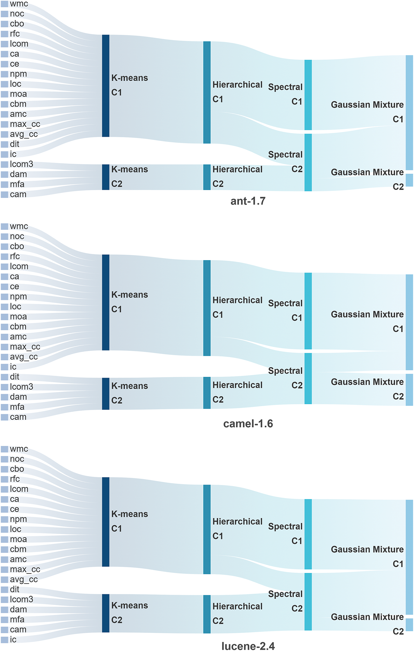
Figure A1: Sankey diagrams of clustering results for the first three projects under four clustering methods

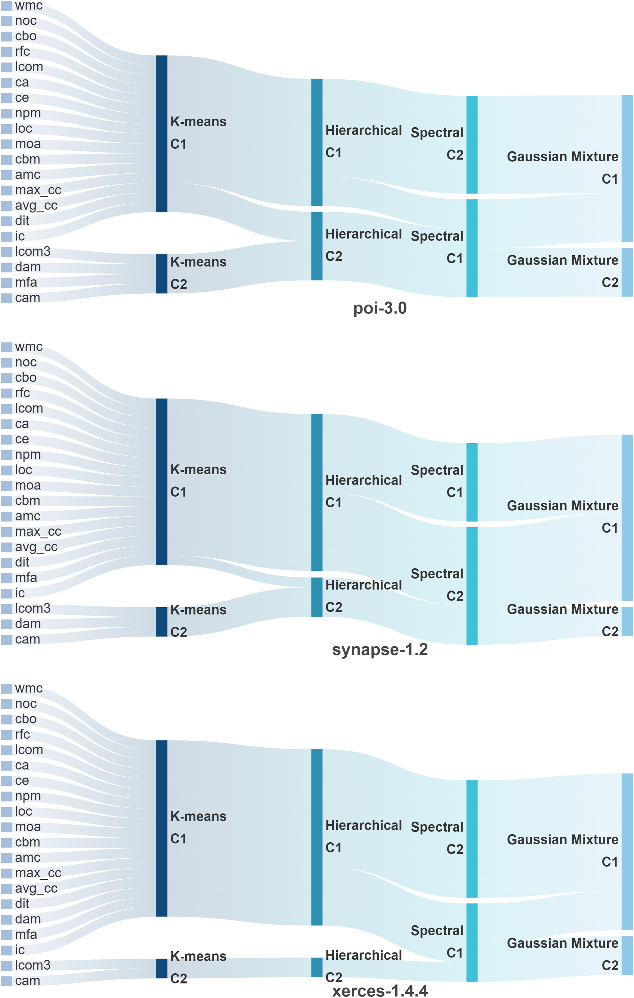
Figure A2: Sankey diagrams of clustering results for the latter three projects under four clustering methods

From Tables A1 to A6, the AUC metric results of different classification models across the three metric groups (Group1, Group2, and Group3) are presented. Similarly, from Tables A7 to A12, the accuracy (Acc) metric results of different classification models under these metric groups are shown.

References

1. Li Z, Jing XY, Zhu X. Progress on approaches to software defect prediction. IET Softw. 2018;12(3):161–75. doi:10.1049/iet-sen.2017.0148. [Google Scholar] [CrossRef]

2. Aranganayagi S, Thangavel K. Clustering categorical data using silhouette coefficient as a relocating measure. In: International Conference on Computational Intelligence and Multimedia Applications (ICCIMA 2007); 2007 Dec 13–15; Sivakasi, India. p. 13–7. [Google Scholar]

3. Abdou AS, Darwish NR. Early prediction of software defect using ensemble learning: a comparative study. Int J Comput Appl. 2018;179(46):29–40. [Google Scholar]

4. Assim M, Obeidat Q, Hammad M. Software defects prediction using machine learning algorithms. In: 2020 International Conference on Data Analytics for Business and Industry: Way Towards a Sustainable Economy (ICDABI); 2020 Oct 26–27; Sakheer, Bahrain. p. 1–6. [Google Scholar]

5. Rahim A, Hayat Z, Abbas M, Rahim A, Rahim MA. Software defect prediction with naïve Bayes classifier. In: 2021 International Bhurban Conference on Applied Sciences and Technologies (IBCAST); 2021 Jan 12–16; Islamabad, Pakistan. p. 293–7. [Google Scholar]

6. Curebal F, Dag H. Enhancing malware classification: a comparative study of feature selection models with parameter optimization. In: 2024 Systems and Information Engineering Design Symposium (SIEDS); 2024 May 3; Charlottesville, VA, USA. p. 511–6. [Google Scholar]

7. Prabha CL, Shivakumar N. Software defect prediction using machine learning techniques. In: 4th International Conference on Trends in Electronics and Informatics (ICOEI); 2020 Apr 16–18; Tirunelveli, India. p. 728–33. [Google Scholar]

8. Matloob F, Ghazal TM, Taleb N, Aftab S, Ahmad M, Khan MA, et al. Software defect prediction using ensemble learning: a systematic literature review. IEEE Access. 2021;9:98754–71. doi:10.1109/access.2021.3095559. [Google Scholar] [CrossRef]

9. Vescan A, Găceanu R, Şerban C. Exploring the impact of data preprocessing techniques on composite classifier algorithms in cross-project defect prediction. Autom Softw Eng. 2024;31(2):47. doi:10.1007/s10515-024-00454-9. [Google Scholar] [CrossRef]

10. Arya A, Malik SK. Design an improved model of software defect prediction model for web applications. In: 2023 International Conference on Artificial Intelligence and Smart Communication (AISC); 2023 Jan 27–29; Greater Noida, India. p. 119–23. [Google Scholar]

11. Zhang F, Zheng Q, Zou Y, Hassan AE. Cross-project defect prediction using a connectivity-based unsupervised classifier. In: 2016 IEEE/ACM 38th International Conference on Software Engineering (ICSE); 2016 May 14–22; Austin, TX, USA. p. 309–20. [Google Scholar]

12. Balogun A, Oladele R, Mojeed H, Amin-Balogun B, Adeyemo VE, Aro TO. Performance analysis of selected clustering techniques for software defects prediction. Afr J Comput ICT. 2019;12(2):30–42. [Google Scholar]

13. Jian Y, Yu X, Xu Z, Ma Z. A hybrid feature selection method for software fault prediction. IEICE Trans Inf Syst. 2019;102(10):1966–75. doi:10.1587/transinf.2019edp7033. [Google Scholar] [CrossRef]

14. Zhou B, Ji J, Gu Z, Zhou Z, Ding G, Feng S. One-step graph-based incomplete multi-view clustering. Multimed Syst. 2024;30(1):32. doi:10.1007/s00530-023-01225-4. [Google Scholar] [CrossRef]

15. Kiyak EO, Birant D, Birant KU. Multi-view learning for software defect prediction. e-Inform Softw Eng J. 2021;15(1):163–84. doi:10.37190/e-inf210108. [Google Scholar] [CrossRef]

16. Chen J, Yang Y, Hu K, Xuan Q, Liu Y, Yang C. Multiview transfer learning for software defect prediction. IEEE Access. 2019;7:8901–16. doi:10.1109/access.2018.2890733. [Google Scholar] [CrossRef]

17. Wang S, Liu T, Nam J, Tan L. Deep semantic feature learning for software defect prediction. IEEE Trans Softw Eng. 2020;46(12):1267–93. doi:10.1109/tse.2018.2877612. [Google Scholar] [CrossRef]

18. Abdu A, Zhai Z, Abdo HA, Algabri R. Software defect prediction based on deep representation learning of source code from contextual syntax and semantic graph. IEEE Trans Reliab. 2024;73(2):820–34. doi:10.1109/tr.2024.3354965. [Google Scholar] [CrossRef]

19. Abdu A, Zhai Z, Abdo HA, Algabri R, Al-Masni MA, Muhammad MS, et al. Semantic and traditional feature fusion for software defect prediction using hybrid deep learning model. Sci Rep. 2024;14(1):14771. doi:10.1038/s41598-024-65639-4. [Google Scholar] [PubMed] [CrossRef]

20. Jureczko M, Madeyski L. Towards identifying software project clusters with regard to defect prediction. In: Proceedings of the 6th International Conference on Predictive Models in Software Engineering; 2010 Sep 12–13; Timisoara. Romania. p. 1–10. [Google Scholar]

21. Kodinariya TM, Makwana PR. Review on determining number of cluster in K-means clustering. Int J. 2013;1(6):90–5. [Google Scholar]

22. Ng A, Jordan M, Weiss Y. On spectral clustering: analysis and an algorithm. Adv Neural Inf Process Syst. 2001;14. [Google Scholar]

23. Hofmann T. Unsupervised learning by probabilistic latent semantic analysis. Mach Learn. 2001;42:177–96. [Google Scholar]

24. Dasgupta S, Long PM. Performance guarantees for hierarchical clustering. J Comput Syst Sci. 2005;70(4):555–69. doi:10.1016/j.jcss.2004.10.006. [Google Scholar] [CrossRef]

25. Chen PH, Lin CJ, Schölkopf B. A tutorial on v-support vector machines. Appl Stochastic Models Bus Ind. 2005;21(2):111–36. doi:10.1002/asmb.537. [Google Scholar] [CrossRef]

26. Breiman L. Random forests. Mach Learn. 2001;45:5–32. [Google Scholar]

27. Chen T, Guestrin C. Xgboost: a scalable tree boosting system. In: Proceedings of the 22nd ACM SIGKDD International Conference on Knowledge Discovery and Data Mining; 2016 Aug 13–17; San Francisco, CA, USA. p. 785–94. [Google Scholar]

28. Taunk K, De S, Verma S, Swetapadma A. A brief review of nearest neighbor algorithm for learning and classification. In: 2019 International Conference on Intelligent Computing and Control Systems (ICCS); 2019 May 15–17; Madurai, India. p. 1255–60. [Google Scholar]

29. Menard S. Applied logistic regression analysis. Thousand Oaks, CA, USA: SAGE Publications; 2001. [Google Scholar]

30. Nitesh VC. SMOTE: synthetic minority over-sampling technique. J Artif Intell Res. 2002;16(1):321. [Google Scholar]

31. Zheng W, Shen T, Chen X, Deng P. Interpretability application of the Just-in-Time software defect prediction model. J Syst Softw. 2022;188(3):111245. doi:10.1016/j.jss.2022.111245. [Google Scholar] [CrossRef]