Simultaneous Depth and Heading Control for Autonomous Underwater Vehicle Docking Maneuvers Using Deep Reinforcement Learning within a Digital Twin System

1  Introduction

The ocean, covering over 70% of the Earth’s surface, offers valuable resources that have driven the increasing deployment of Autonomous Underwater Vehicles (AUVs) for safe and efficient exploration and development. AUVs are widely utilized for a variety of tasks, including seabed resource exploration, marine habitat monitoring, and deep-sea structure inspections [1,2]. Their high safety, reliability, and controllability make them indispensable in missions such as seabed mapping [3], underwater equipment inspection [4], and mine detection [5]. As underwater missions become more complex and prolonged, long-term endurance has become a critical requirement for AUV operations. To meet this demand, underwater docking stations have been developed to provide power recharging and data transmission capabilities, which are essential for extending mission duration and enhancing autonomy. However, achieving reliable docking remains a significant challenge. Environmental uncertainties such as ocean currents, limited visibility, and posture deviations between the AUV and docking station introduce substantial difficulties for precise motion control during docking maneuvers [6,7]. Although vision-based guidance systems, such as the one proposed by Li et al. [8], have improved docking accuracy and achieved up to 80% success rates, many early studies were limited by controlled test environments and simplified motion models. These constraints have restricted the applicability of such methods to fully autonomous and precise docking operations in more dynamic and unpredictable underwater settings.

With the development of hardware like cameras, visual information has become a crucial source for decision-making and judgment in AUV monitoring and identification tasks. DL has improved image processing, making image recognition for docking missions widely adopted. Singh et al. [9] used YOLO (short for You Only Look Once) to identify the LED light rings of target docking stations for positioning. Sans-Muntadas et al. [10] employed a Convolutional Neural Network (CNN) to map camera inputs to error signals for controlling the docking of AUVs, demonstrating the feasibility of autonomous docking using only camera lenses as sensors.

The AUV docking process comprises the return and docking phases, with a reliable return control system crucial for successful docking. Li et al. [6] developed a hybrid method integrating ultra-short baseline and computer vision to enhance accuracy and stability during final docking. Standard controllers, such as PID and fuzzy controllers, are capable of controlling a stable, fast and accuracy performance. However, with the nonlinear nature of underwater environments, the performance of fixed parameters can be limited [11]. In this case, machine learning (ML) is increasingly applied to AUV control strategies. Reinforcement Learning (RL) has gained prominence for its ability to learn through environmental interactions and feedback, improving performance over traditional methods. Yu et al. [12] demonstrated that DRL offers superior accuracy in AUV trajectory tracking compared to PID methods.

To overcome the inherent limitations of conventional PID methods in dealing with nonlinear and uncertain underwater environments, the sigmoid PID controller incorporates nonlinear modulation through a sigmoid function, which significantly improves control adaptability and stability [13]. BELBIC PID controllers, inspired by brain emotional learning, have been employed to manage dynamic behaviors in AUVs more effectively [14]. Neuroendocrine PID controllers, integrating neural networks with endocrine mechanisms, have also demonstrated robustness under uncertain conditions [15]. Although these intelligent PID controllers improve adaptability and control precision, they still require extensive parameter tuning and exhibit limited generalization across diverse scenarios. Their ability to handle highly dynamic, unstructured environments, such as those encountered in autonomous docking, remains constrained.

In recent years, deep reinforcement learning (DRL) has attracted significant attention in the field of AUV control, offering promising solutions for complex and dynamic underwater environments. The Deep Deterministic Policy Gradient (DDPG) algorithm, which combines Deep Q-Network (DQN) techniques with an Actor-Critic architecture to output deterministic actions, has demonstrated its ability to handle continuous state and action spaces effectively [16]. Carlucho et al. [17] applied DDPG to address AUV path navigation, while Yao and Ge [18] further enhanced the method by incorporating an adaptive multi-restrictive reward function, achieving better results in three-dimensional path tracking and obstacle avoidance. Despite its advantages, DDPG presents limitations such as instability in policy updates and overestimation of action-value functions, which hinder its reliability in more challenging scenarios. To overcome these issues, Fujimoto et al. [19] proposed the Twin Delayed Deep Deterministic Policy Gradient (TD3) algorithm, introducing twin critics, delayed policy updates, and target policy smoothing to stabilize learning and improve control accuracy. Li and Yu [20] later applied TD3 for real-time trajectory planning in multi-AUV charging navigation, ensuring timely and collision-free arrival at charging stations. Beyond DRL approaches, recent studies have explored hybrid control strategies. For instance, an adaptive PID controller based on Soft Actor–Critic (SAC) has been proposed to enhance interpretability and performance in AUV path following tasks [21]. Additionally, the integration of fuzzy logic with PID control has been investigated to address nonlinearities and uncertainties in AUV dynamics [22]. Model Predictive Control (MPC) methods have also been advanced, with recent work incorporating Gaussian Processes to improve trajectory tracking and obstacle avoidance capabilities in dynamic ocean environments [23]. These developments underscore the rapid evolution of control techniques for AUVs. However, while these methods perform well in simulated settings, further integration with digital twin (DT) systems remains necessary to ensure robust and reliable transfer to real-world docking operations.

In addition to DRL, several advanced tuning algorithms have been proposed to optimize controllers in nonlinear systems. The Memorizable Smoothed Functional Algorithm (MSFA) enhances convergence and reduces computational cost through memory-based search [24], while Norm-Limited Simultaneous Perturbation Stochastic Approximation (NL-SPSA) stabilizes gradient estimates for systems with nonlinearities [25]. Smoothed functional variants have also improved reinforcement learning convergence in off-policy tasks [26]. However, these methods mainly target static or simplified scenarios and remain limited in handling sequential decision-making and sim-to-real transfer, which are essential for AUV docking. Compared to these approaches, DRL algorithms offer distinct advantages in addressing sequential decision-making and sim-to-real transfer challenges, which are critical for AUV docking in dynamic underwater environments.

Underwater vehicle performance is affected by payload and environmental changes, complicating parameter design and accurate mathematical modeling. Additionally, advancements in image recognition have outpaced simple numerical simulations, leading to increased focus on developing high-fidelity simulation environments. Manhães et al. [27] proposed an Unmanned Underwater Vehicle (UUV) simulator based on the open-source robot simulation platform Gazebo. This simulator allows for collaborative task simulations for multiple AUVs and simulates underwater operation interaction tasks using robotic arms. However, the visual quality of UUV Simulator is relatively low, makes it lacks authenticity when processing image. Henriksen et al. [28] proposed an open-source simulator for underwater vehicles, MORSE. This simulator supports ROS and Python, making it suitable for academic research and sensor simulation. However, it has relatively simple graphics, and its underwater physics engine lacks accuracy. Potokar et al. [29] proposed HoloOcean, an open-source underwater vehicle simulator based on Unreal Engine 4 (UE4). This simulator can be easily installed through simple steps and quickly execute simulations through the Python interface, with reliable physics engine and visual quality. It also allows easy construction of the required underwater environment within the UE4 software.

This study establishes a DT system characterized by synchronized interaction between the physical and virtual environments and the transfer of control algorithms from simulation to real-world applications (sim-to-real transfer). The digital twin system in this study is defined based on the triad architecture proposed by Grieves [30]. Sharma et al. [31] noted that DT technology offers advantages such as real-time monitoring, simulation, optimization, and accurate prediction, but its theoretical framework and practical applications have not yet been widely realized. Liu et al. [32] established a DT system for a physical robot using DT technology to transfer DRL algorithms to real-world robots. Their experimental results confirmed the effectiveness of intelligent grasping algorithms and the virtual-to-real transfer methods and mechanisms based on digital twins.

Recently, DT technology has been increasingly applied in various fields [33], further demonstrating its potential to bridge virtual models with real-world systems. Additionally, several studies have made notable progress in advancing DT technologies and reinforcement learning methods for underwater robotics. Chu et al. [34] proposed an adaptive reward shaping strategy to enhance DRL for AUV docking, addressing the challenges of complex environmental dynamics. Patil et al. [35] systematically benchmarked several DRL algorithms for underwater docking, confirming the effectiveness of TD3 in achieving high success rates, yet their work remained limited to simulation environments without full sim-to-real validation. Chu et al. [36] introduced MarineGym, a reinforcement learning benchmark platform designed for underwater tasks, which emphasized training efficiency and reproducibility, but did not focus on docking or transfer to real-world applications. Yang et al. [37] integrated DT technology with reinforcement learning for autonomous underwater grasping, demonstrating the potential of sim-to-real transfer, albeit in tasks other than docking. Havenstrøm et al. [38] investigated DRL-based control for AUV path following and obstacle avoidance, yet without incorporating DT systems or addressing docking scenarios.

This study aims to build an asynchronous AUV digital twin simulation system as an initial step toward a complete DT system, addressing limitations in real-time underwater communication. After evaluating various open-source platforms, HoloOcean was selected to develop the 3D AUV simulation system, using the UE4 engine to simulate 6-DOF motion and visualize vehicle movement. Experimental hydrodynamic coefficients were integrated into the model to ensure realistic simulation results. Although DRL and simulation platforms have been widely adopted in AUV control studies, most remain limited to purely simulated environments without addressing the gap to real-world operations. To overcome this limitation, this study proposes a DT system that integrates the physics-based simulation platform and DRL algorithms, enabling not only control strategy training but also seamless sim-to-real transfer. The developed controllers were successfully validated in real AUV docking experiments, demonstrating the practicality and reliability of our approach. Thus, the system serves both as a DRL training environment and as a bridge to real-world deployment. This research not only enhances AUV control but also provides insights for future AUV digital twin development.

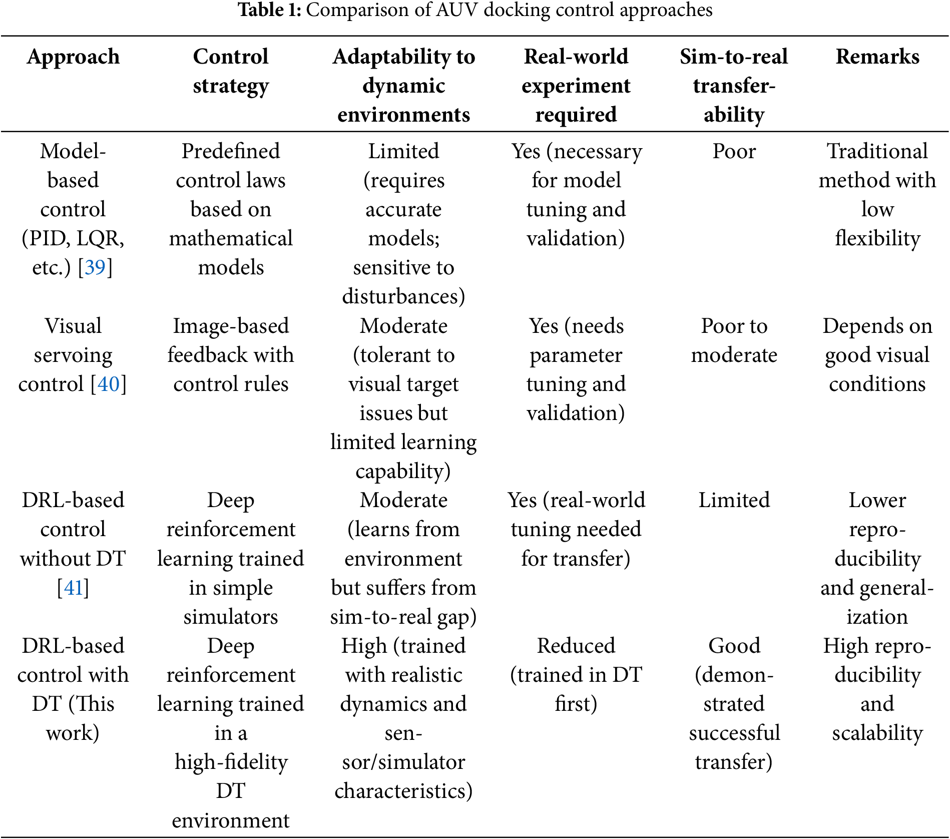
Table 1 summarizes the differences between the proposed method and other state-of-the-art approaches for AUV docking control. Compared to conventional methods relying on hand-crafted control laws or visual servoing techniques, our DT-based DRL control system offers improved adaptability, reduced dependency on real-world trials, and demonstrated robustness through successful sim-to-real transfer. This comparative analysis highlights the potential of the proposed approach as a scalable and efficient solution for autonomous underwater docking missions.

This study proposes a DT system integrated with DRL to achieve adaptive and transferable AUV docking control. A hybrid control strategy combining TD3 and a novel image-based I-DDPG is developed and successfully validated through both simulation and real-world experiments, demonstrating robust sim-to-real transfer. Furthermore, comprehensive quantitative evaluations confirm the reliability and effectiveness of the proposed method in handling nonlinear and uncertain underwater environments. The remainder of this study is organized as follows: Section 2 elaborates on the methodologies related to AUVs, docking devices, and DRL-based continuous motion control. Section 3 outlines the framework of the 3D AUV maneuvering system. In Section 4, the control methods and experimental design are introduced. Section 5 validates the feasibility of the simulation and experimental results, along with the data analysis. Finally, Section 6 concludes the study and discusses future work.

2  Methodology

To accurately describe the motion of the AUV, it is necessary to define coordinate systems, including the earth-fixed coordinate system and the body-fixed coordinate system, as shown in Fig. 1. [u,v,w,p,q,r] represents the linear and angular velocities relative to the body-fixed coordinate system, while [x,y,z] denotes the AUV’s position in the earth-fixed coordinate system. The Euler angles ϕ, θ, and ψ refer to the AUV’s orientation relative to the earth-fixed coordinate system.

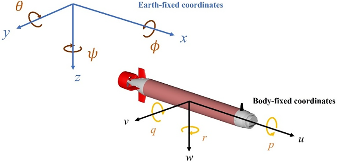
Figure 1: The schematic of the earth-fixed and body-fixed coordinate systems

2.1 Design of MateLab AUV

The MateLab AUV features capabilities such as image identification, 6-DOF motion control, depth-keeping, and heading stabilities. The AUV’s hull design is based on the model proposed by Myring [42], with a total length of 1.7 m and a diameter of 0.17 m, resembling a torpedo shape, as shown in Fig. 2a. It weighs 40 kg, with positive buoyancy adjusted to 0.15 kg to ensure it can float to the surface in case of a system shutdown. The AUV is composed of three sections: the bow compartment, the control compartment, and the stern compartment. The bow compartment is equipped with a wide-angle camera, a stereo camera module, LED lights, and a pressure sensor module; the control compartment houses a mini-industrial computer, batteries, and various control modules; the stern compartment features propulsion provided by a DC brushless motor paired with a four-blade propeller and includes four independent servos for rudder operation, with each rudder’s axis control range being ±30°. Detailed configurations are illustrated in Fig. 2b. In this study, the mini-industrial computer integrates several key modules through serial communication methods such as RS232. These modules include the depth measurement module, the attitude and heading reference system (AHRS), the imaging module, the Bluetooth module, the propulsion control system, and the power management system, as shown in Fig. 2c.

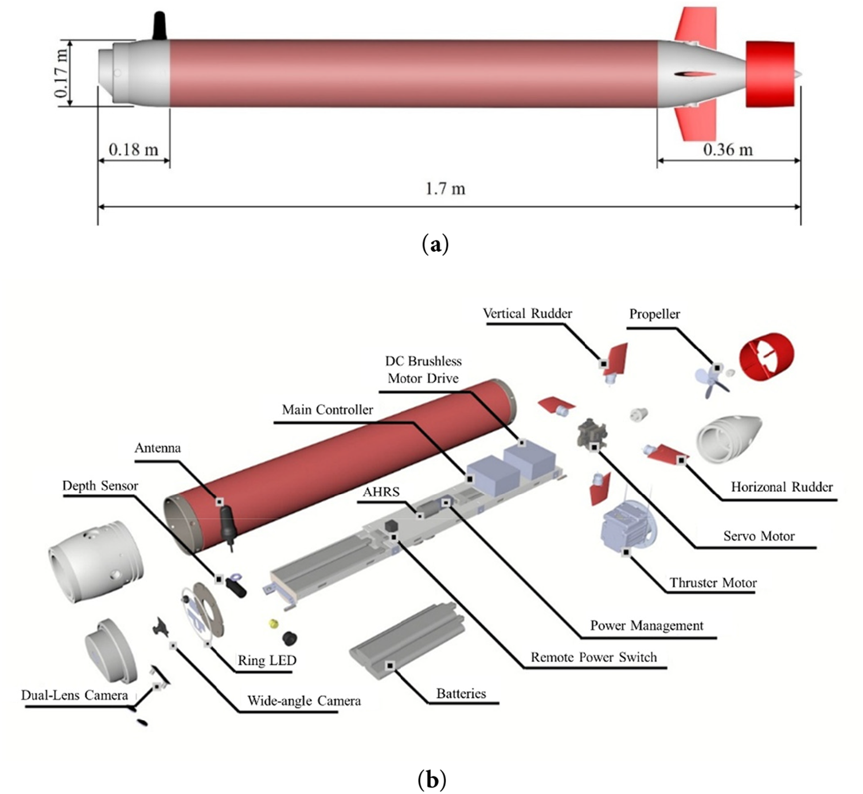
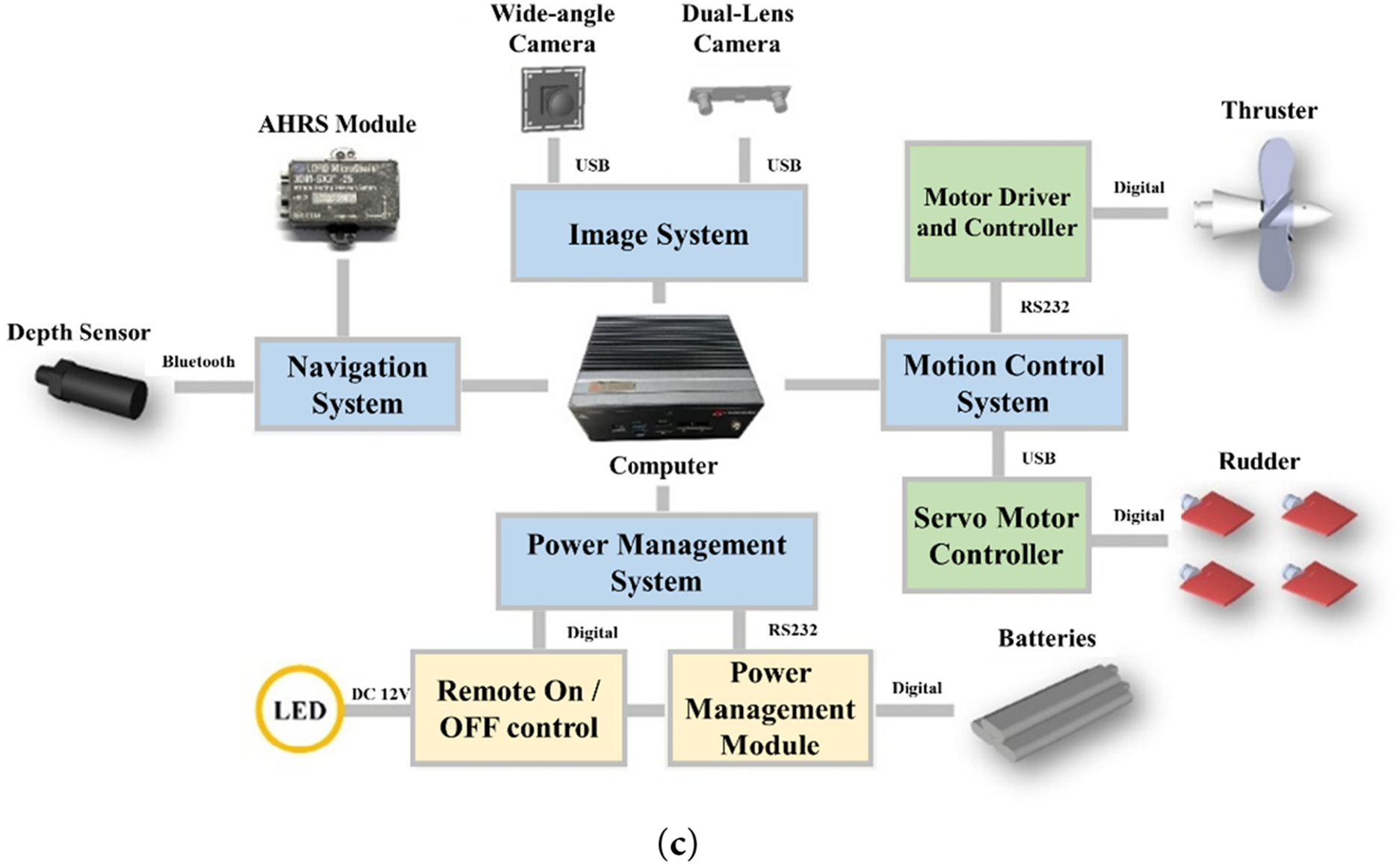
Figure 2: MateLab AUV: (a) geometric appearance; (b) internal configuration diagram; (c) comprehensive system block diagram

2.2 Equation of Motion for AUV

The motion model of an AUV integrates rigid-body dynamics with kinematic equations, typically expressed using hydrodynamic coefficients. The vehicle’s motion is primarily influenced by factors such as body inertia, hydrodynamic forces, propeller thrust, and rudder forces. The hydrodynamic coefficients vary depending on hull type and operational conditions, and their selection is often based on empirical determination. This study employs the six-degree-of-freedom motion equation model proposed by Fossen [43], as represented in Eq. (1).

Mν˙+C(ν)ν+D(ν)ν+g(η)=τ(1)

where M represents the system inertia matrix of the AUV (including added mass), C(v) denotes the Coriolis-centripetal matrix (including added mass), D(v) is the damping matrix of the AUV, g(η) represents the restoring force and moment matrix due to gravity and buoyancy, and τ represents the vector of control input. Since ν represents the velocity state vector of the AUV in the body-fixed coordinate system, while η denotes the position and orientation state vector in the Earth-fixed coordinate system, a transformation between these two representations is required.

(1)   System inertia matrix

The system inertia matrix M is defined in Eq. (2). Assuming the AUV is fully submerged, M is positive definite and constant.

M=MRB+MA,M=MT>0,M˙=0(2)

The matrix M comprises the rigid-body system inertia matrix MRB and the added mass system inertia matrix MA, which are defined in Eq. (3).

MRB=[m000mzg−myg0m0−mzg0mxg00mmyg−mxg00−mzgmygIx−Ixy−Izxmzg0−mxg−IxyIy−Iyz−mygmxg0−Izx−IyzIz](3)

MA=[−Xu˙−Xv˙−Xw˙−Xp˙−Xq˙−Xr˙−Xv˙−Yv˙−Yw˙−Yp˙−Yq˙−Yr˙−Xw˙−Yw˙−Zw˙−Zp˙−Zq˙−Zr˙−Xp˙−Yp˙−Zp˙−Kp˙−Kq˙−Kr˙−Xq˙−Yq˙−Zq˙−Kq˙−Mq˙−Mr˙−Xr˙−Yr˙−Zr˙−Kr˙−Mr˙−Nr˙]

where m represents the total mass of the vehicle; Ix,Iy,Iz denote the mass moments of inertia of the vehicle relative to the body-fixed coordinate system along the respective axes of rotation; xg,yg,zg denote the position of the AUV’s center of gravity. The added mass system inertia matrix MA is composed of the vehicle’s hydrodynamics coefficients. Relevant symbols and parameters are listed in the Nomenclature. Since the AUV used in this study is symmetrical about the vertical axis, yg=Ixy=Iyz=0, and the matrix M can be simplified as shown in Eq. (4).

M=[m−Xu˙0−Xw˙0m−Yv˙0−Xw˙0m−Zw˙0−mzg−Yp˙0mzg−Xq˙0−mxg−Zq˙0mxg−Yr˙00mzg−Xq˙0−mzg−Yp˙0mxg−Yr˙0−mxg−Zq˙0Ix−Kp˙0−Izx−Kr˙0Iy−Mq˙0−Izx−Kr˙0Iz−Nr˙](4)

(2)   Coriolis-centripetal matrix

The Coriolis-centripetal matrix C(v) arises from the rotational coupling between the Earth-fixed and body-fixed coordinate systems, as defined in Eq. (5). For a rigid body moving through an ideal fluid, C(v) is parameterized to exhibit skew symmetry.

C(ν)=CRB(ν)+CA(ν)(5)

C(ν)=−CT(ν),ν∈R6

The matrix C(v) comprises the rigid-body Coriolis-centripetal matrix CRB(v) and the added mass Coriolis-centripetal matrix CA(v), where CA(v) represents the fluid forces induced by the rigid body’s motion through an ideal fluid. The matrices CRB(v) and CA(v) are defined in Eqs. (6a,b).

CRB(ν)=[000000000−m(ygq+zgr)m(ygp+w)m(zgp−v)m(xgq−w)−m(zgr+xgp)m(zgq+u)m(xgr+v)m(ygr−u)−m(xgp+ygq)(6a)

m(ygq+zgr)−m(xgq−w)−m(xgr+v)−m(ygp+w)m(zgr+xgp)−m(ygr−u)−m(zgp−v)−m(zgq+u)m(xgp+ygq)0−Iyxq−Ixzp+IzrIyzr+Ixyp−IyqIyxq+Ixzp−Izr0−Ixzr−Ixyq+Ixp−Iyzr−Ixyp+IyqIxzr+Ixyq−Ixp0]

CA(ν)=[0000−Zw˙wYv˙v000Zw˙w0−Xu˙u000−Yv˙vXu˙u00−Zw˙wYv˙v0−Nr˙rMq˙qZw˙w0−Xu˙uNr˙r0−Kp˙p−Yv˙vXu˙u0−Mq˙qKp˙p0](6b)

(3)   Damping matrix

The fluid dynamic damping in an AUV is inherently nonlinear and coupled. To approximate the damping matrix D(v), it is commonly assumed to be diagonal, comprising the products of damping coefficients and their respective velocity components, as shown in Eq. (7).

D(ν)=−[X|u|u|u|000000Y|v|v|v|000Y|r|r|r|00Z|w|w|w|0Z|q|q|q|0000K|p|p|p|0000M|w|w|w|0M|q|q|q|00Y|v|v|v|000N|r|r|r|](7)

(4)   Restoring force and moment matrix

The matrix g(η) represents the restoring forces and moments of the AUV, arising from gravity and buoyancy, as defined in Eq. (8). WAUV denotes the weight acting on the AUV, while BAUV represents the buoyancy force. The coordinates xb,yb,zb indicate the position of the AUV’s buoyancy center, whereas xg,yg,zg denote the position of its center of gravity.

g(η)=[(WAUV−BAUV)sin⁡θ−(WAUV−BAUV)cos⁡θsin⁡ϕ−(WAUV−BAUV)cos⁡θcos⁡ϕ−(ygWAUV−ybBAUV)cos⁡θcos⁡ϕ+(zgWAUV−zbBAUV)cos⁡θsin⁡ϕ(zgWAUV−zbBAUV)sin⁡θ+(xgWAUV−xbBAUV)cos⁡θcos⁡ϕ−(xgWAUV−xbBAUV)cos⁡θcosϕ−(ygWAUV−ybBAUV)sin⁡θ](8)

(5)   Control input vector

In this study, the AUV regulates its attitude using two vertical and two horizontal control fins, complemented by a thruster. Establishing a mapping between the vehicle control inputs and the resulting forces and moments is therefore essential. This research adopts the control input model proposed by Harris and Whitcomb [44]. The position of the ith fin in the vehicle frame is denoted by piV, as defined in Eq. (9).

piV=|riVϕiV|∈R6(9)

where riV denotes the vector from the vehicle’s center to the center of the ith fin, and ϕiV represents the angular position of the ith fin in the vehicle frame.

(6)   AUV Hydrodynamics

By substituting Eqs. (2) and (5) into Eqs. (1), (10) is obtained:

MRBν˙+CRB(ν)ν=τ−MAν˙−CA(ν)ν−D(ν)ν−g(η)(10)

where the left-hand side represents the inertial forces and moments acting on the AUV, while the right-hand side comprises external forces, including hydrodynamic forces, restoring forces, and control inputs. The hydrodynamic forces and moments acting on the AUV, denoted by FHD6×1, are expressed in Eq. (11):

FHD6×1=−MAν˙−CA(ν)ν−D(ν)ν(11)

The hydrodynamic force components along six degrees of freedom are expanded in terms of dimensionless hydrodynamic coefficients, as presented in Eqs. (12)–(17). These equations enable the calculation of hydrodynamic forces and moments acting on the AUV across six degrees of freedom.

Surge:

FHD1=ρ2L4[Xqq′q2+Xrr′r2+Xrp′rp]+ρ2L3[Xu˙′u˙+Xvr′vr+Xwq′wq]+ρ2L2[Xuu′u2+Xvv′v2+Xww′w2](12)

Sway:

FHD2=ρ2L4[Yp˙′p˙+Yr˙′r˙+Ypq′pq+Yp|p|′p|p|]+ρ2L3[Yv˙′v˙+Ywp′wp+Yv|r|′v|v||(v2+w2)12||r|+Ypup+Yrur]+ρ2L2[Yuu′u2+Yv′uv+Yv|v|′v|(v2+w2)12|+Ywvwv](13)

Heave:

FHD3=ρ2L4[Zq˙′q˙+Zrr′r2+Zrp′rp]+ρ2L3[Zw˙′w˙+Zvr′vr+Zvp′vp]+ρ2L3[Zq′uq+Zw|q|′w|w||(v2+w2)12||q|]+ρ2L2[Zuu′u2+Zw′uw+Zw|w|′w|(v2+w2)12|]+ρ2L2L2[Z|w|′u|w|+Zww′|w(v2+w2)12|+Zvv′v2](14)

Roll:

FHD4=ρ2L5[Kp˙′p˙+Kr˙′r˙+Kqr′qr+Kp|p|′p|p|]+ρ2L4[Kp′up+Kr′ur+Kv˙′v˙+Kwp′wp]+ρ2L3[Kuu′u2+Kv′uv+Kvw′vw+Kv|v|′v|(v2+w2)12|](15)

Pitch:

FHD5=ρ2L5[Mq˙′q˙+Mrr′r2+Mrp′rp]+ρ2L4[Mq′uq+M|w|q′|(v2+w2)12|q+Mw˙′w˙+Mvr′vr+Mvp′vp]+ρ2L3[Muu′u2+Mw′uw+Mw|w|′w|(v2+w2)12|]+ρ2L3[M|w|′u|w|+Mww′|w(v2+w2)12|+Mvv′v2](16)

Yaw:

FHD6=ρ2L5[Nr˙′r˙+Npq′pq+Np˙′p˙]+ρ2L4[Nr′ur+N|v|r′|(v2+w2)12|r+Np′up+Nv˙′v˙+Nwp′wp]+ρ2L3[Nuu′u2+Nv′uv+Nv|r|′|(v2+w2)12|+Nwv′wv](17)

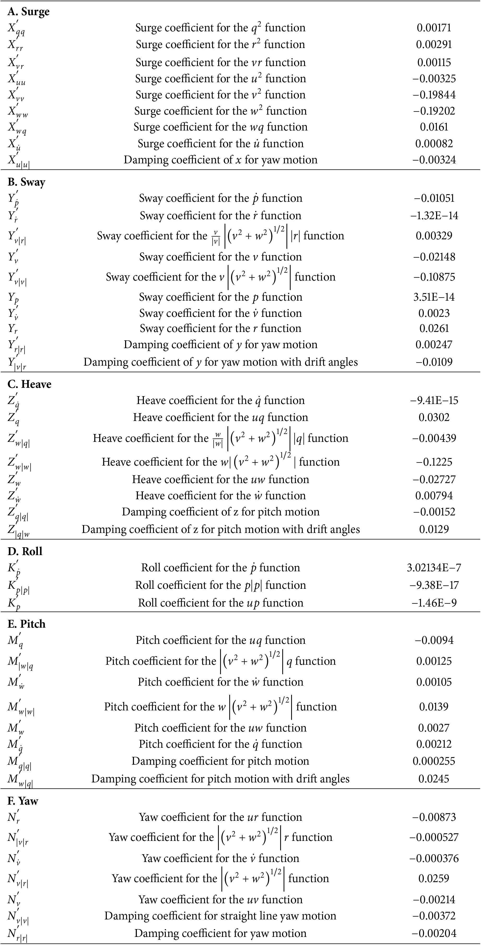
The right-hand sides of the equations present the expanded forms of the hydrodynamic forces expressed in terms of dimensionless hydrodynamic coefficients. ρ denotes the fluid density, and L represents the vehicle length. The hydrodynamic coefficients adopted in this study are based on our previous study [45], which established the coefficients through towing tank experiments and validated the model’s accuracy in reproducing real AUV motion responses. The details of these coefficients are provided in Appendix A.

2.3 The Docking System

The docking system offers an effective solution to recovering the AUV to the mother ship, providing greater flexibility and ease of repositioning compared to more expensive fixed docking systems. The movable docking system is illustrated in Fig. 3. This study utilizes our developed docking device featuring a rectangular frame as its main structure. The conical docking entrance is constructed from aluminum alloy bars, with an opening at the top to accommodate an antenna or sail. The rear end is equipped with an adjustable support bracket, allowing it to accommodate AUVs of various lengths. The entrance is equipped with LED ring lights to serve as targets for AUV visual recognition and positioning tracking. Additionally, a fixed bracket for a variable information light disc is positioned above the entrance, though this study focuses on using the LED ring for docking information.

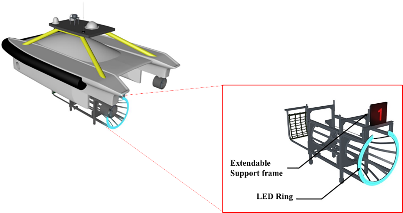
Figure 3: The schematic of the movable docking system

2.4 YOLOv7 Deep Learning Object Recognition Algorithm

YOLO [46] differs from traditional object detection models by framing the object detection problem as a single regression task, combining all aspects of object detection into one unified neural network. This approach enables YOLO to detect and locate all objects in an image in a single pass, offering faster and more comprehensive inferences on the entire image while predicting both the categories and locations of objects. Building upon YOLOv4, Wang et al. [47] introduced the YOLOv7 algorithm with several enhancements and optimizations. YOLOv7 adopts a different CNN structure, incorporating extended efficient layer aggregation networks (ELAN) and model scaling techniques to improve both inference speed and accuracy. The processing flow of the YOLO algorithm is illustrated in Fig. 4.

Figure 4: Illustration of the YOLO processing flow

To adapt the YOLOv7 model for underwater docking scenarios, a domain-specific dataset was created using synthetic images from the UE4-based digital twin environment and real-world images from basin experiments. The dataset included various perspectives and lighting conditions of the docking station’s LED light ring. The YOLOv7 model, initialized with COCO-pretrained weights, was subsequently fine-tuned on this dataset. Through transfer learning and hyperparameter tuning, the model achieved a balance between detection accuracy and real-time performance, enabling robust target localization during the docking maneuvers. This study applies the YOLOv7 object detection method to achieve target recognition and localization in docking missions, serving as the perception module within the I-DDPG control system.

2.5 DRL-Based Continuous Motion Control

DRL utilizes deep neural networks to approximate value functions or control policies, improving learning accuracy and enabling applications in more complex interactive environments. This study employs two DRL algorithms, DDPG and TD3, for docking control and depth-heading control in docking tasks.

2.5.1 The Architecture and Algorithm of DDPG

The DDPG algorithm is a DRL method specifically designed for continuous control problems. Based on the Actor-Critic framework, DDPG utilizes deep neural networks and policy gradient methods to output deterministic actions, making it well-suited for continuous action spaces and high-dimensional state spaces. The architecture of the DDPG network is illustrated in Fig. 5, where the temporal difference error (TD-error) represents the discrepancy between the predicted and target values.

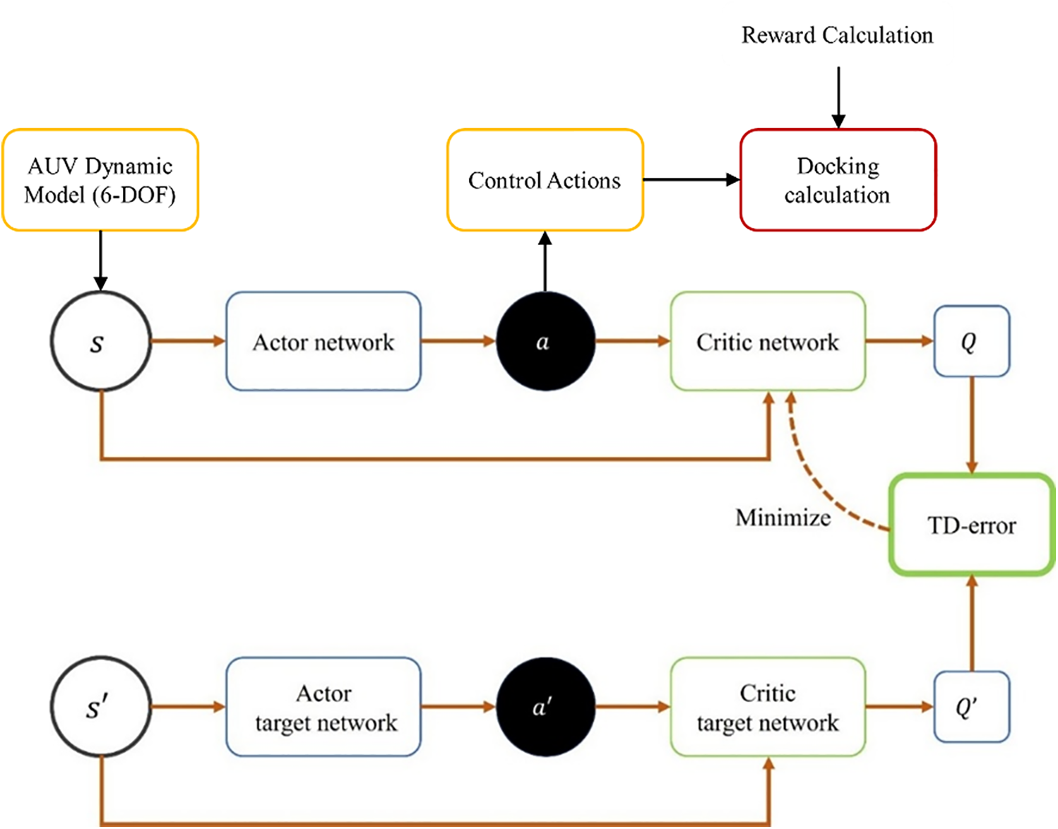
Figure 5: The architecture of the DDPG network

2.5.2 The Architecture and Algorithm of TD3

DDPG has been successfully applied to many continuous control problems. However, it faces challenges such as unstable policy updates and overestimation of Q-values. To address these issues, Fujimoto et al. [19] proposed the TD3 algorithm. TD3 is an optimized version of DDPG, incorporating three key improvements: target policy smoothing, clipped double-Q Learning, and delayed policy updates. Target policy smoothing enhances algorithm stability by smoothing the target Q-values, clipped double-Q learning prevents overly optimistic value estimates, improving policy reliability, and delayed policy updates reduce fluctuations in the policy network, enhancing learning stability. These enhancements enable TD3 to demonstrate superior performance across various control tasks, particularly in applications such as robotics control, autonomous driving, and game AI.

As shown in Fig. 6, the TD3 agent in this study follows a similar framework to DDPG for continuous AUV control, where AUV motion states serve as input to the Actor-Critic networks. The agent outputs control actions that directly command the rudder and thruster, forming the control inputs to the AUV dynamic model. The closed-loop interaction is reinforced through reward feedback, enabling the DRL agent to learn effective control policies suited for underwater docking tasks.

Figure 6: The network architecture of TD3

3  AUV Simulation and Control System Architecture

In this study, an integrated 3D AUV simulation and control system was developed using the open-source underwater robot simulator HoloOcean, which is based on the reinforcement learning simulator Holodeck [48] and Unreal Engine 4 (UE4). UE4 offers a robust platform that provides accurate physics simulation, high-fidelity visual rendering, and flexible environment customization through its C++ and Blueprint interfaces. By using these capabilities, the proposed simulation system integrates the AUV motion model as the core simulation component and serves as the virtual environment for DRL training and control validation, as illustrated in Fig. 7. In this system architecture, the AUV receives control commands, rudder deflection angles (δV,δH) and thruster speed (rpmthrust), directly from the DRL agent implemented in Python. These control actions are applied to the AUV dynamic model within the simulation, which computes the resulting motion states at the next time step, including velocities and orientations ([u,v,w,p,q,r,X,Y,Z,ϕ,θ,ψ]). The updated states are then fed back to the DRL agent as observations, forming a closed-loop control cycle that enables continuous policy learning and refinement. This simulation and control integration not only supports efficient DRL training, but also ensures that the learned control policies are aligned with the dynamic behaviors of the real AUV, thus enhancing sim-to-real transferability. This simulation platform serves as the DT environment for AUV control development, fulfilling the real-time feedback loop between simulation and physical experimentation.

Figure 7: Architectural diagram of the digital twin system environment

3.1 Motion Simulation in HoloOcean

The numerical integration method commonly used in physics engines to approximate these results is the semi-implicit Euler method. It combines the simplicity of the explicit Euler method with the stability of the implicit Euler method, providing a balance of low computational cost and stability. Therefore, in HoloOcean, external forces such as buoyancy, gravity, and propeller thrust are applied to the AUV model in each frame, as shown in Fig. 8. The physics engine then computes the AUV’s position and attitude based on these applied forces, simulating the AUV’s motion through this process.

Figure 8: Schematic of the HoloOcean simulation method

3.2 UE4 Visualization and AUV Simulation Setup

First, the 3D model of the AUV needs to be imported into UE4, and its surface materials must be configured (as shown in Fig. 9a) to closely match its real-world appearance. The sensor modules, including the forward-looking camera, depth sensor, and INS, are then positioned according to the actual AUV system architecture. By utilizing UE4’s terrain tools and water plugins, a realistic underwater environment can be created. This study employs the capabilities of the UE4 game development platform to construct the virtual underwater environment used in the simulation system, as shown in Fig. 9b.

Figure 9: (a) 3D model of the AUV in UE4; (b) the virtual underwater environment

After importing the model into UE4, interaction functionalities can be implemented either by editing character blueprints or using C++. In this study, the AUV model is developed using C++ code. The initial step involves setting the basic specification parameters of the AUV, including the center of gravity, center of buoyancy, weight, and volume. Additionally, the positions of the propeller and rudder need to be set, as they will be used to apply propeller thrust and rudder forces, respectively. The positions of the center of buoyancy and center of gravity are defined relative to the vehicle’s coordinate center.

This study employs the numerical simulation method [49] for the AUV, using hydrodynamic equations to compute the hydrodynamic forces [FHD1,FHD2,FHD3,FHD4,FHD5,FHD6] acting on the AUV. To ensure the fidelity of the simulation environment, the DT system integrates multiple sources of real-world data. Experimental hydrodynamic coefficients, derived from prior towing tank tests [45], were embedded into the simulation model to replicate realistic underwater dynamics. In addition, sensor characteristics, including camera parameters, pressure sensor accuracy, and AHRS update rates, were incorporated to emulate real sensor performance. Finally, by enabling the ‘Simulate Physics’ feature within the character blueprint, the PhysX physics engine is used to solve for the AUV’s velocity, angular velocity, position, and attitude. The computed data is then rendered into visual imagery using the GPU. Furthermore, the results from real-world AUV docking experiments were used to validate and fine-tune the simulation outputs, establishing a continuous feedback mechanism that enhances the accuracy and reliability of the digital twin framework. The basic parameters are determined by referencing the previously established AUV numerical motion model descripted in Section 2.2, which creates a numerically accurate model of the AUV in UE4 environment.

3.3 Simulation System Interface and Workflow

The Python interface of HoloOcean in this study emulates the design of OpenAI Gym [50], enabling simulations to be executed with only a few lines of code. This environment facilitates parameter adjustment, data collection and integration, simulation control, DRL training, and result output. Action commands are transmitted from Python to the simulation system, which subsequently computes the AUV’s state information for the next time step. The computed state information is returned to Python, serving as input for the DRL model during training. Furthermore, data displayed on the simulation window provides real-time feedback on the current simulation status of the AUV. The simulation process is illustrated in Fig. 10.

Figure 10: Simulation process of the Python interface

4  Control Methods and Experimental Design

The AUV’s docking process is divided into three stages: positioning (surface sailing and diving states), searching (depth-keeping and searching states), and docking (object-tracking state), enabling the AUV to locate the docking device and complete the docking task. This study focuses on evaluating the control performance of the DT system during this planned docking process and its virtual-to-real conversion. For the positioning and searching stages, the TD3 algorithm is implemented to control both the depth and heading of the AUV. The input states include real-time depth, pitch, and yaw angles, while the actions consist of horizontal and vertical rudder commands. The reward function is designed to minimize depth and heading errors while maintaining smooth control. Except for the docking stage, TD3 is employed for horizontal plane heading control and vertical plane depth control, as illustrated in Fig. 11a. During the docking stage, the I-DDPG algorithm is applied, using the bounding box coordinates of the detected target object as input states to generate rudder control commands. The reward structure focuses on target alignment accuracy while penalizing abrupt actions to ensure stable docking maneuvers. The overall control process and transition among the stages are depicted in Fig. 11b.

Figure 11: (a) Diagram of AUV control stages; (b) process of the docking task

TD3 adopts two critic networks to mitigate Q-value overestimation by averaging the outputs, thereby enhancing stability and accuracy. In contrast, DDPG uses a single critic network, which may lead to overestimation and less stable learning. This structural difference allows TD3 to outperform DDPG, particularly in complex environments. During the searching stage, both the thruster and rudder require high-precision control, whereas in the docking stage, only the rudder is needed once the AUV is sufficiently close to the dock. Detailed discussions on each method are presented in the following sections.

4.1 TD3 Depth and Heading Control Method

In the positioning stage, when the target is out of visibility range and cannot be tracked, specifically during the surface sailing and diving states, this study uses depth information (h) obtained from the pressure sensor and the pitch angle (θ) and yaw angle (ψ) obtained from the AHRS as inputs to the TD3 model. This allows the AUV to simultaneously maintain heading control while diving to the target depth. In such a complex task involving synchronized control in both the horizontal and vertical planes, DRL is particularly advantageous. It can determine the optimal control actions under various states, enabling the AUV to approach the target’s visibility range with a stable posture.

To achieve stable depth and heading control during the positioning stage, this study utilizes the proposed maneuvering simulation system to train TD3 to control the AUV during this phase. In the simulation environment, the AUV’s initial position is set at the origin of the world coordinates with the bow oriented at a heading angle of 0∘. At the beginning of the simulation, the AUV is in an unstable state. Therefore, each round begins with a 10-s stabilization period to allow the AUV to reach a stable state before starting the 60-s control operation. To maintain stable depth and heading control during the positioning stage, this study sets tracking targets in both the vertical and horizontal planes: a target depth of 0.7 m and a target heading angle of 0∘.

The training process of interacting TD3 with the AUV 3D maneuvering simulation system is illustrated in Fig. 12. In each step, the agent generates a set of horizontal and vertical rudder angle actions a based on the input AUV depth and attitude state s. The action is then input into the simulation environment, producing the next state s′, the reward value r calculated according to the reward function, and the signal d indicating whether the episode has ended. This data (s,a,r,s′,d) is immediately stored in the replay buffer. These steps are repeated 60 times in each training episode, with each episode considered one voyage. Unlike DDPG, TD3 does not wait for the replay buffer to be filled before updating; instead, it begins updating the network parameters as soon as the number of data points exceeds the set batch size and continues until the training is complete.

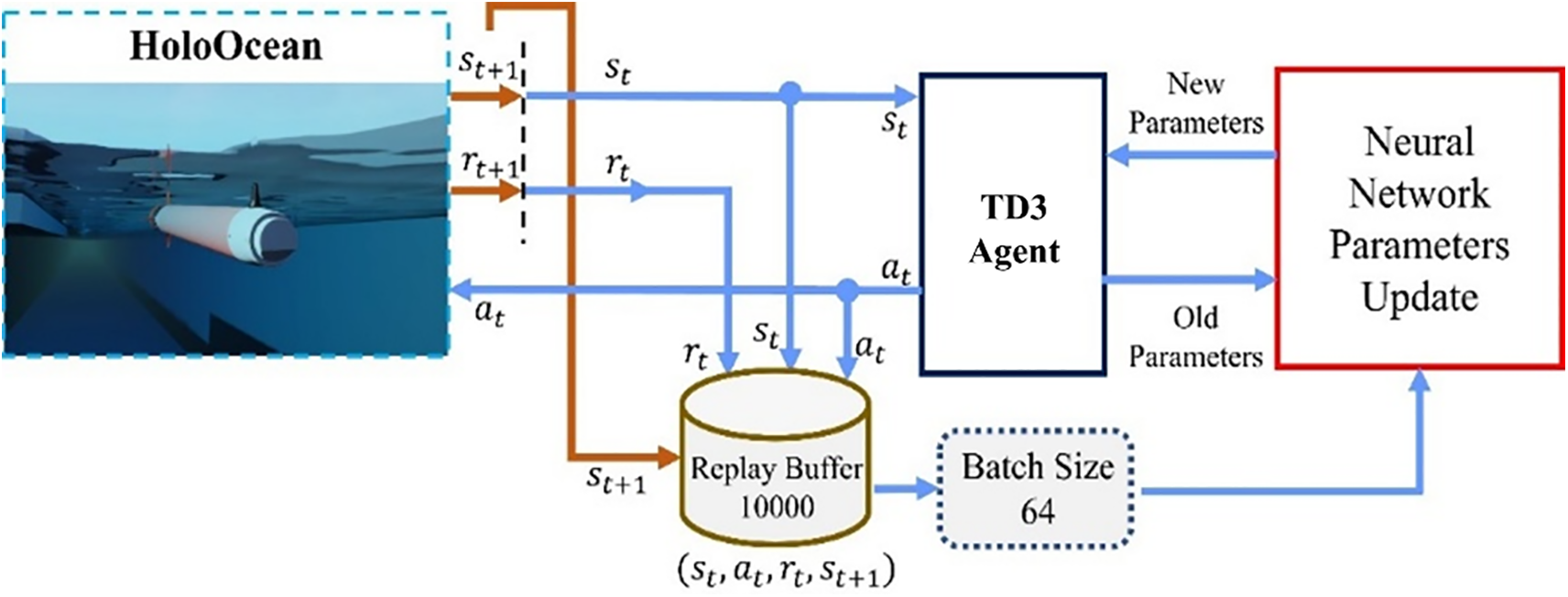
Figure 12: TD3 training process

During the TD3 training process, the environmental states consist of the AUV’s current depth information (h), pitch angle (θ), and yaw angle (ψ). These pieces of information form the basis for TD3’s control decisions. The output actions are the angles of the AUV’s horizontal rudders (δH) and vertical rudders (δV). The reward function of the TD3 model was designed to achieve stable and accurate control during the positioning and searching stages. To this end, the reward formulation considers depth error, heading angle error, and control effort (rudder angles), aiming to minimize deviations from the target states while encouraging smooth and stable control actions. The specific design of the reward function is shown in Eq. (18).

rT=rh+eδH+rψ+ry

rh={10⋅(0.05−Δh)0.05,Δh≤0.05 mmax(−10,−10⋅(Δh−0.05)0.05),Δh>0.05 m,Δh=|h−htarget|

eδH={−10,h≤0.15 and |ΔδH|≥15∘0,else

ry={10⋅(0.05−Δy)0.05,Δy≤0.05 mmax(−10,−10⋅(Δy−0.05)0.05),Δy>0.05 m,Δy=|y−ytarget|(18)

Δψ0.5∘=0.5∘⋅xbow180∘π,Δψ=|ψ(t)−ψtarget|⋅xbow180∘π

rψ={10⋅(Δψ0.5∘−Δψ)Δψ0.5∘,Δψ≤Δψ0.5∘max(−10,−10⋅(Δψ−Δψ0.5∘)Δψ0.5∘),Δψ>Δψ0.5∘

where rT represents the total reward. rh is the reward value for depth, with higher values indicating closer proximity to the target depth. eδH is a penalty applied based on the actual situation to prevent excessive horizontal rudder angles during navigation, as this could cause the AUV’s tail to rise and reduce propulsion speed. rψ is the reward value for the yaw angle, where smaller changes in the yaw angle indicate more stable navigation. The yaw angle is multiplied by xbow180∘π to convert the yaw angle error into the swept arc length. xbow is the distance from the bow to the center of gravity, measured at 1.05 m. ry is the reward value for lateral distance, which helps in better understanding the AUV’s heading control performance.

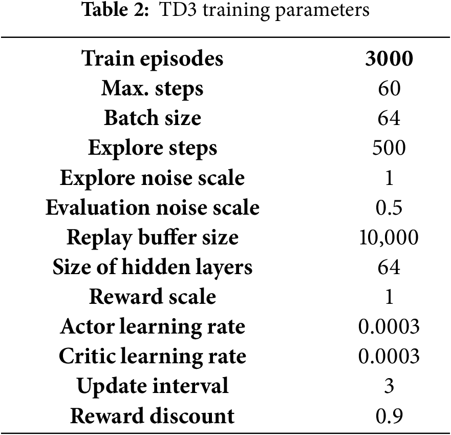
The training parameters are listed in Table 2. The model is trained for 3000 episodes, which is deemed sufficient for learning various environmental features based on the complexity of the task. Each episode has a maximum of 60 steps, which is appropriate for the target docking task. The batch size for updates is set to 64, striking a balance between training stability and computational efficiency. The reward discount factor, γ, is set to 0.9, prioritizing long-term rewards while preventing premature convergence to short-term solutions. The number of initial random action explorations is set to 500 steps, allowing the model to explore diverse possibilities and mitigate the risk of local minima. Action noise, implemented using Gaussian noise, is introduced to enhance action diversity and improve the robustness of the learned policy. The learning rates for both the actor and critic networks are set at 0.0003, with the Adam optimizer employed for parameter updates to ensure stable and efficient convergence.

4.2 I-DDPG Image Target Tracking Control Method

This study employs the I-DDPG method as the docking control approach during the docking stage. I-DDPG is a DRL algorithm based on DDPG, which integrates Image-based Visual Servoing (IBVS) object detection as the target input. In this study, the YOLO algorithm is employed for detecting the target LED ring. The tracking process of the I-DDPG control is illustrated in Fig. 13a. After the camera captures images of the target, YOLO is used for identification and localization, obtaining target information, including the bounding box center coordinates and dimensions (TU,TV,wb,hb), as shown in Fig. 13b. The image resolution is 1280 × 720 pixels, and all four parameters are normalized by dividing the pixel coordinates by the image resolution. The normalized target image information is then used as the state input for the I-DDPG image target tracking model, forming the basis for the control decisions of the AUV’s rudder actions (aD) to track and dock with the target device. The action aD consists of two elements: δV, representing the vertical rudder angle, and δH, representing the horizontal rudder angle. Specific settings are detailed in Table 3. The reward function is designed to minimize the distance between the target bounding box center and the image center, while also penalizing excessive rudder actions to ensure smooth control performance.

Figure 13: (a) Process of I-DDPG image-object-tracking control; (b) illustration of the target located within the AUV’s field of view

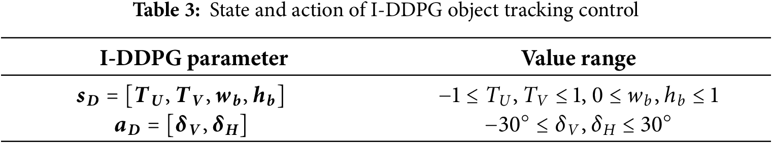
To ensure the successful docking of the AUV with the target dock, the goal is to keep the target object as close to the center of the AUV’s camera frame as possible by controlling [δV,δH]. Accordingly, the reward function was designed to reflect visual tracking performance and control smoothness. It rewards the AUV for aligning the target LED ring close to the center of the camera’s field of view, while penalizing sudden or large rudder adjustments to maintain smooth motion. In addition, failure to detect the target is heavily penalized to drive the policy towards reliable and continuous object detection. These design principles ensure that the AUV can precisely and steadily complete the docking process. The reward function used in the training process is designed as shown in Eq. (19).

rT=rA+ro+rδV+rδH+rb+rX

ro={0,Object is detected−10,Object is not detected

rδV={1,|δV|≤Thresr−|δV|−2.52.5,|δV|>Thresr(19)

rδH={1,|δH|≤Thresr−|δH|−2.52.5,|δH|>Thresr

rb={−10,|Y|≥4m or Z<−3.4m0,else

rX=XDock−XAUV4

where rA represents the reward for the target object’s position, determined based on the region where the center coordinates [TU,TV] are located. The closer these coordinates are to the center of the image, the higher the reward value, as illustrated in Fig. 14. ro denotes the negative reward associated with target detection. If YOLOv7 fails to detect the target object, it is considered to be outside the image range, and a significant negative reward is assigned to discourage this scenario. rδV and rδH are the rewards based on the rudder angle. Positive rewards are given if the AUV maintains stable navigation with a smaller rudder angle during tracking. Conversely, negative rewards are assigned to discourage excessive rudder angles, which could lead to oscillations in the navigation path, thereby enhancing navigation stability. The rudder angle threshold, denoted as Thresr, is set to 10∘. rb represents the negative reward given when boundary conditions are triggered to prevent the AUV from colliding with obstacles or reaching the bottom. rX is the reward for the distance to the target object, with higher rewards given as the AUV approaches the docking device.

Figure 14: Illustration of the reward based on the target object’s position

I-DDPG is built upon the DDPG algorithm and is trained within the visualization simulation environment combining Unity and MATLAB. At each step, the model determines the angles for the horizontal and vertical rudders, denoted as at, based on the input environmental state st, and receives the next state st+1 along with the reward rt. The interaction results (st,at,rt,st+1) are stored in the Replay Buffer. This process is repeated until the episode reaches the maximum number of steps or the AUV reaches the target location. Before the Replay Buffer is sufficiently populated with data, the parameters of the decision network and evaluation network are not updated. Once a sufficient amount of data is collected, 32 samples are randomly drawn from the Replay Buffer to update and optimize the network parameters. After training, model weight files for the decision network and evaluation network are generated. These files can then be loaded into the AUV control program to perform target tracking tasks. The training process flowchart is illustrated in Fig. 15.

Figure 15: Interactive illustration of I-DDPG and digital twin

The training parameters for I-DDPG are presented in Table 4. The complexity of the environment states and the high-dimensional action space in the target tracking task necessitate long training times for convergence. Consequently, the number of training episodes was set to 3000. As illustrated in Fig. 16, which depicts the relationship between reward values and the number of episodes, the reward value begins to increase toward a local maximum only after approximately 500 episodes. Subsequently, the reward values continue to fluctuate before stabilizing at around 2500 episodes. To alleviate convergence difficulties arising from this complexity, the size of the experience replay buffer was reduced, enabling more frequent updates to the network parameters and thereby accelerating the convergence rate.

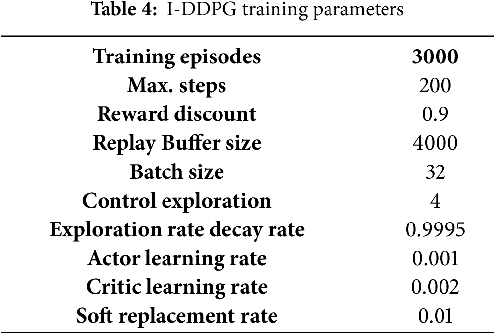
Figure 16: Variation in the reward during the I-DDPG training process

4.3 Design of the Underwater Docking Experiment

To validate the control effectiveness of the TD3 controller, which was trained using the developed 3D AUV maneuvering simulation system for tracking target depth and heading control, and to assess its impact on the subsequent docking stage, this study conducted both simulations and practical experiments on an AUV underwater docking task. The practical experiments were carried out in a water basin at National Cheng Kung University, measuring 50 m in length, 25 m in width, and with a water depth of 2 m.

The equipment setup for the underwater docking task in this study is as follows: The center of the docking device’s entrance was submerged to a depth of 1 m below the water surface, with the initial distance for the task set at 50 m. Both the simulation and experimental environments were configured according to these parameters. The simulation environment was based on the maneuvering simulation system, as shown in Fig. 17a. The key difference between the actual experiment and the simulation is that the experimental environment does not include a movable platform. As a result, only the docking device was placed in the water during the experiment. The docking device remained afloat due to its buoyancy, provided by the attached floats. By adjusting the position of these floats, the center of the docking device’s entrance was maintained at a depth of 1 m below the water surface. The experimental environment setup is illustrated in Fig. 17b.

Figure 17: The equipment setup in (a) the simulation environment, and (b) the experimental environment

5  Result and Discussion

In the underwater docking task, TD3 is applied to control the depth and heading during the positioning stage, enabling the AUV to stably descend to a position suitable for searching the docking device. During the searching stage, zig-zag heading motion control is used in combination with YOLOv7 to capture the position of the docking device. In the final docking process, the I-DDPG image target control system is used to navigate the AUV toward the docking device and adjust its posture to align with the target device. Subsequently, the feasibility of TD3 is validated by comparing simulation and experimental results. Eventually, the total performance and stability of the docking task will be evaluated via automatic docking experiments and data analysis.

5.1 Training Results of TD3 for Synchronous Control of Depth and Heading

This study utilizes a maneuvering simulation system to train TD3 for simultaneous depth and heading control. This training process optimizes the controller for horizontal and vertical rudder adjustments during the positioning stage of the subsequent underwater docking task. Fig. 18 illustrates the variation in reward values throughout the training process. Due to the complexity of achieving simultaneous control in both horizontal and vertical planes, this continuous control task presents significant challenges for the convergence of the reward function. It is not until after 1500 episodes that the reward values increase significantly and converge to a higher value range. Despite this, significant fluctuations remain in the later stages of training.

Figure 18: Variation in the reward during the TD3 training process

After 3000 training episodes, the TD3 model demonstrates effective performance in controlling both depth and heading in a real-world system experiment. Fig. 19a–c illustrates the time series for depth (h), pitch angle (θ), and horizontal rudder angle (δH) for vertical plane control of the AUV. Fig. 19d–f presents the results of horizontal plane control, including the relationship between lateral displacement (y) and distance (x), the time series of yaw angle (ψ), and vertical rudder angle (δV). The depth results in Fig. 19a indicate that the TD3 model successfully stabilizes the AUV at the target depth. Fig. 19b shows that the AUV maintains a smooth pitch angle during diving and converges to stability in the depth-keeping state. However, the horizontal rudder angle in Fig. 19c indicates that the model generates suboptimal control actions with reduced smoothness due to the reward function not incorporating action smoothness. Fig. 19d presents the XY-plane trajectory, and Fig. 19e shows the yaw angle, both confirming that the AUV effectively maintains the target heading throughout its journey. Finally, Fig. 19f shows that the vertical rudder angle exhibits fluctuations, which are similarly attributed to the reward function’s design not incorporating action smoothness.

Figure 19: Training results for TD3 depth and heading control: (a) AUV’s depth; (b) pitch angle; (c) horizontal rudder angle; (d) XY plane position; (e) yaw angle; (f) vertical rudder angle

The depth control performance of the TD3 model can be compared with that of other studies. Lin et al. [51] conducted an AUV depth-keeping study using an adaptive fuzzy controller, which demonstrated AUV depth-keeping performance with a target depth of 1 m. The red line in Fig. 20 represents the depth-keeping performance of the TD3 controller, while the blue line represents that of the adaptive fuzzy controller. The presented data is normalized with respect to the target depth. The results clearly show that the TD3 controller enables the AUV to reach the target depth faster and maintain stability more effectively than the adaptive fuzzy controller.

Figure 20: Comparison between the TD3 controller and the adaptive fuzzy controller (htar: Target depth)

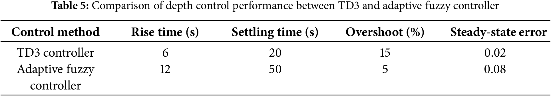
It should be noted that the response of the TD3 controller is displayed over a 60-s period, which corresponds to the typical duration of the positioning and searching stages. Within this time frame, the controller’s transient response, convergence speed, and steady-state accuracy can be sufficiently demonstrated. Furthermore, this duration reflects practical constraints imposed by the physical dimensions of the test environments, including the towing tank and plane water basin. Additionally, a zoom-in subplot has been added to highlight the transient response within the first 60 s, where performance differences are most pronounced. In general, Fig. 20 indicates the superior performance of the TD3 controller in terms of response speed and depth-keeping stability, achieving 25% less oscillation than the adaptive fuzzy controller when reaching the target depth, which highlights its enhanced stability, accuracy, and potential scalability for more complex autonomous underwater tasks.

In addition to the qualitative comparison illustrated in Fig. 20, a quantitative analysis has been conducted to further evaluate the performance of the TD3 controller. Table 5 summarizes key time response specifications, including rise time and settling time, calculated from the depth control experiments. These indicators provide a more detailed assessment of the controller’s dynamic performance and stability. Moreover, as shown in the experimental results, the TD3-based control method achieves faster convergence and better steady-state accuracy compared to the conventional adaptive fuzzy controller. This clearly demonstrates the superiority of the proposed method in handling complex underwater docking tasks.

5.2 Simulation and Experimental Results of AUV Underwater Docking

Prior to conducting the actual underwater docking experiments, this study first designed and simulated the entire docking control process using a maneuvering simulation system. The subsequent underwater docking experiments were conducted following this planned process to validate both the TD3 model’s control capability in real underwater environments and the feasibility of the planned task flow in simulation, as illustrated in Fig. 21a,b. The docking process was divided into the following stages: 0–15 s for positioning, 15–50 s for searching (transitioning earlier to docking if the target is detected), and 50 s onward for docking.

Figure 21: The recodes of (a) simulation, and (b) experiments

Fig. 22a–g presents the recorded data from the underwater docking task simulation and actual experiments, including yaw angle (ψ), depth (h), pitch angle (θ), vertical rudder angle (δV), horizontal rudder angle (δH), and the horizontal (TU) and vertical (TV) coordinates of the detected target center in the image. In Fig. 22a, the yaw angles during the first 15 s of the positioning stage show similar patterns across all experimental cases, consistent with the simulation results. This is due to the AUV’s single-propeller propulsion system, where surface sailing causes the pitch angle to expose part of the propeller above water, generating a lateral force at the tail and resulting in a leftward yaw deviation. For depth control, as shown in Fig. 22b, both the simulation and experiments demonstrate successful diving. However, the experiments took longer to stabilize at the target depth compared to the simulation, as the simulation did not account for the propeller emerging from the water, which in reality reduces thrust efficiency. The pitch angle results in Fig. 22c show significant changes when the AUV reached the target depth, prompting TD3 to apply large corrective horizontal rudder angles (Fig. 22d), resulting in overshoot in the simulation. While this affected depth-holding performance, TD3 still stabilized the AUV at a fixed depth with minimal pitch deviations in both the simulation and experiments during the searching stage. Although Fig. 22e shows TD3 attempting to correct the yaw deviation by adjusting the rudder to the right, this correction was limited as half of the vertical rudder was exposed above water, reducing its effectiveness. Fig. 22f indicates that the AUV successfully adjusted its position toward the center of the image frame. In Fig. 22g, the target object’s vertical coordinates remained centered in the image during the simulation. However, in the experiments, since the docking device was positioned at a depth of 1 m, the target object appeared only in the upper portion of the image when viewed from a distance. To maintain stable navigation, the control logic was adjusted to place the target object at the upper horizontal center of the image, around pixel position (640, 90). This result confirms that all experimental cases successfully adjusted the vertical coordinate of the target object to align with the revised center.

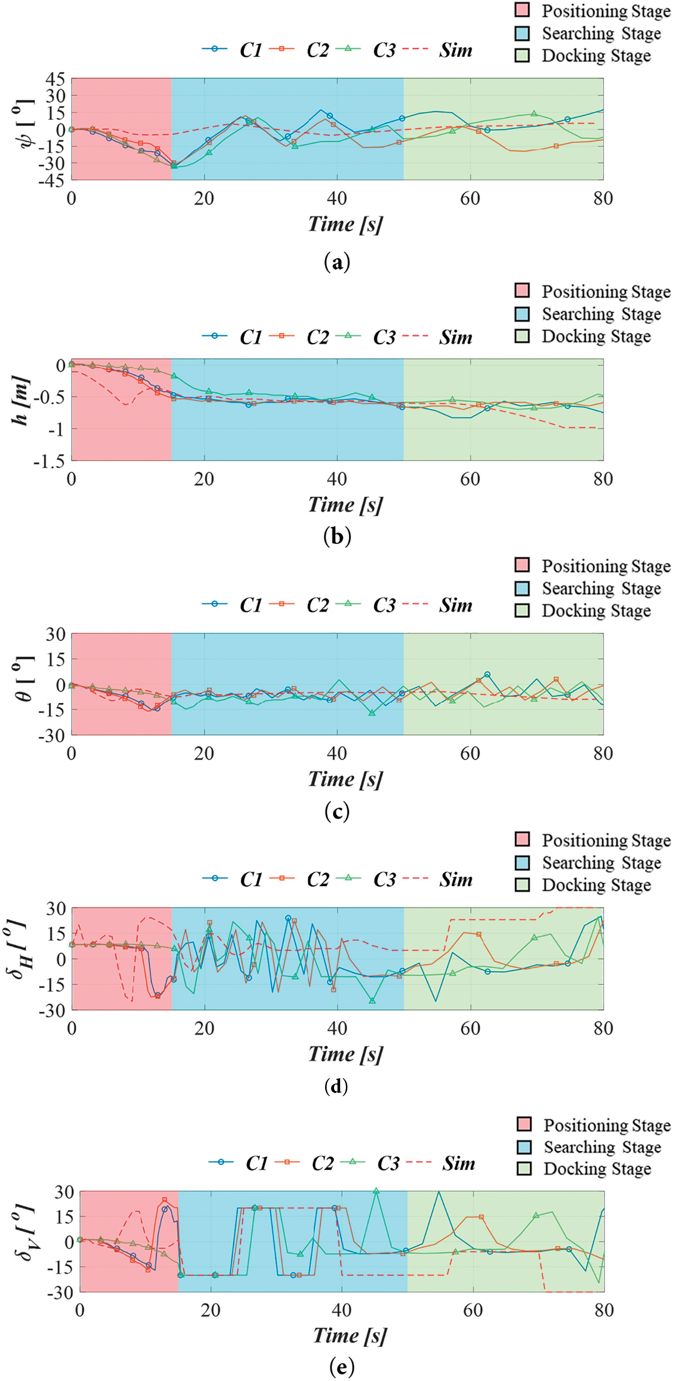
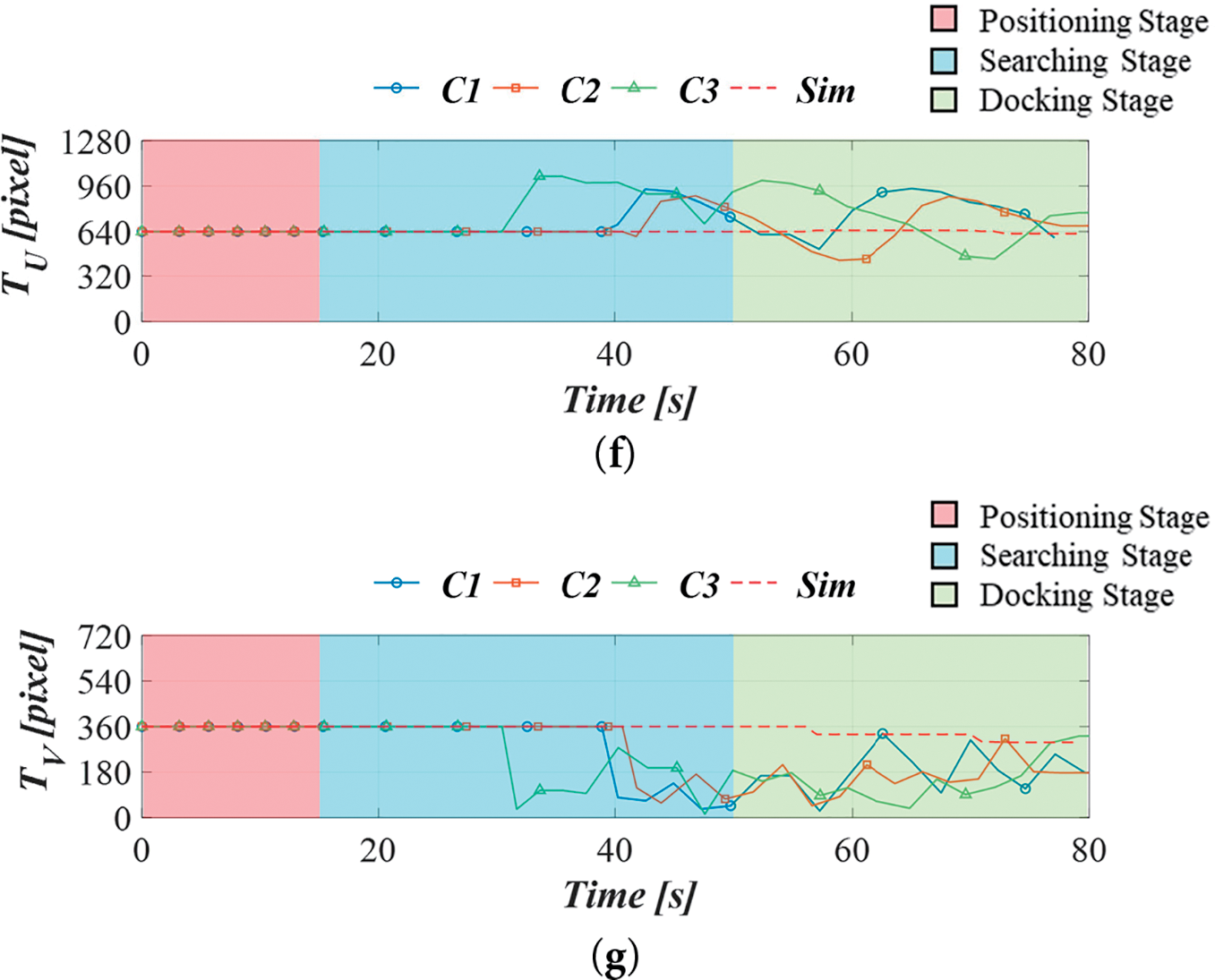
Figure 22: Time series of AUV’s docking tasks: (a) yaw angle; (b) depth; (c) pitch angle; (d) horizontal rudder angle; (e) vertical rudder angle; (f) horizontal image coordinate of the target; (g) vertical image coordinate of the target

5.3 Data Analysis

In this study, TD3 was employed for the synchronous control of depth and heading angle during the positioning stage. In the searching stage, TD3 continued to control depth, while heading control was switched to the zig-zag method. The effectiveness of these control strategies was evaluated by plotting the depth and heading angle distributions in the visual coordinate system for both the simulation and all experimental cases during the positioning and searching stages, as shown in Fig. 23a–d. The horizontal axis represents the AUV’s heading angle (ψ), the vertical axis represents the depth (h), and the color bar represents the temporal evolution of the AUV’s position. In Fig. 23a, the simulation begins at 0 s and continues until the planned 50 s, before the simulation transitions to the docking control phase. During this period, the AUV steadily dives to the predetermined depth and maintains the heading angle within the pre-set range throughout the searching phase. Fig. 23b–d shows that, despite initial heading deviations in all experimental cases, the AUV successfully dives to a stable depth and maintains the heading angle within the pre-set range as dictated by the searching strategy. Finally, in C1, C2, and C3, the target was detected at 39, 40, and 30 s, respectively, resulting in an earlier transition to the docking control phase.

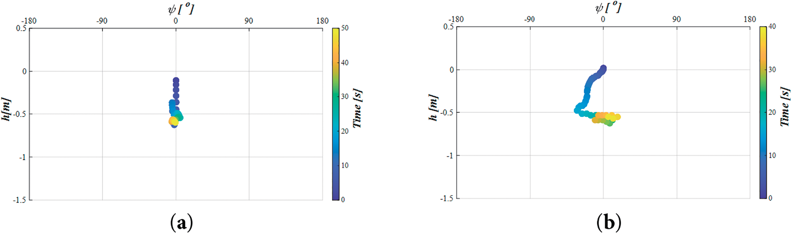
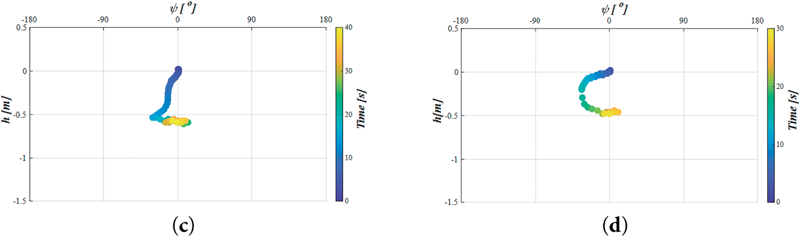
Figure 23: Distributions of depth (h) and yaw angle (ψ) during the positioning and searching stages in (a) simulation; (b) C1; (c) C2; and (d) C3

In this study, image coordinates were used as the main control parameters during the docking stage. The tracking results were evaluated based on the distribution of the target image center on visual coordinates for both the simulation and all experimental cases during the docking stages, as shown in Fig. 24a–d. The horizontal axis represents the image’s horizontal coordinate (TU), the vertical axis represents the image’s vertical coordinate (TV), and the color bar indicates time. Red boxes mark the 25% and 50% areas of the image center, showing different distribution intervals within the image coordinates. Due to adjustments in the control logic, the image center coordinates shifted upwards during the experiment, moving from the dashed section to the solid section, as shown in Fig. 24b–d. Fig. 24a shows that during the entire docking stage in the simulation, the target image center coordinates were consistently maintained within the 25% area. This is because there were no significant heading deviations during the simulation’s searching phase, and the depth-maintaining posture was stable with a relatively small pitch angle. Fig. 24b–d demonstrates that, although the target image center distribution was not as concentrated as in the simulation, it generally remained within the 50% area in all experimental cases. As the AUV approached the docking device, the coordinates were corrected to within the 25% area. This discrepancy might be related to inferences regarding thrust, inertia, and resistance, which could have caused greater oscillations in the AUV’s posture during the docking control phase, affecting the stability of the docking process.

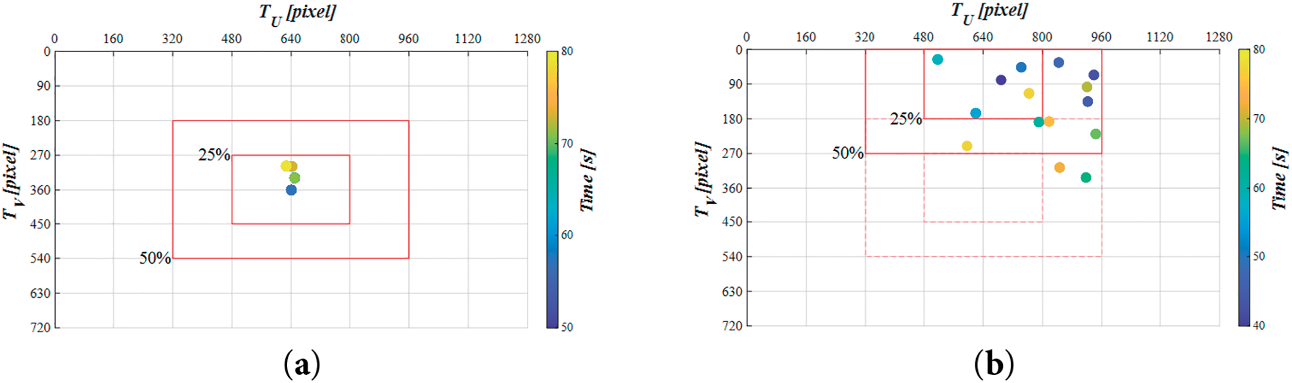
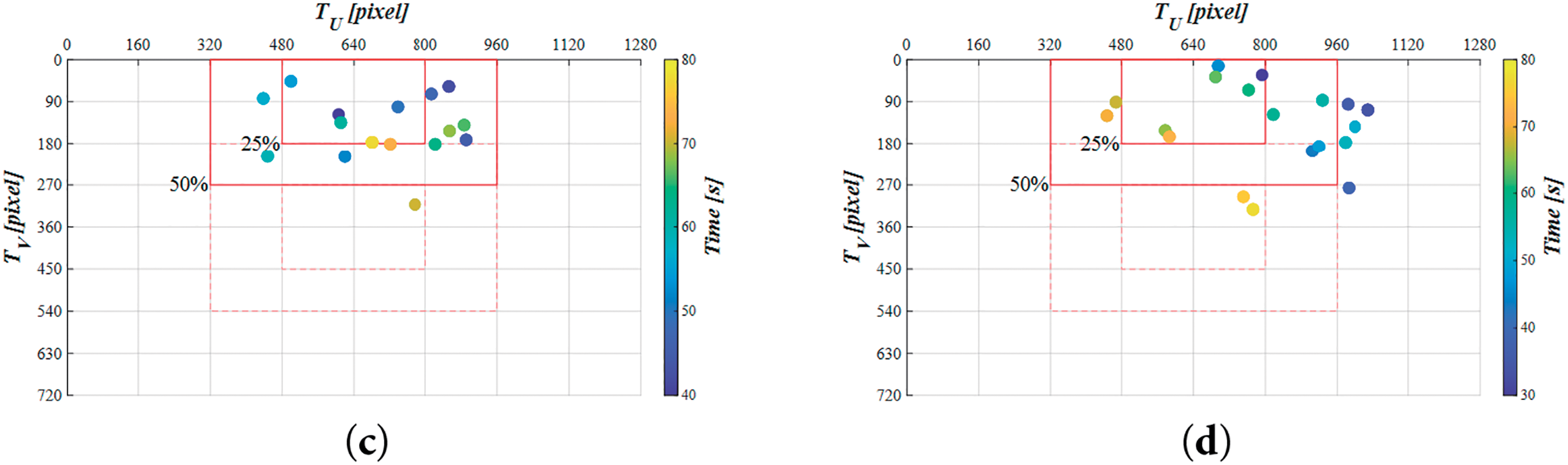
Figure 24: Trajectory of the dock’s image center in the image coordinate system during the docking stage in (a) the simulation, (b) C1, (c) C2, and (d) C3

The docking initiation times in the simulation and all experimental cases varied due to differences in image recognition results. Therefore, only the first 15 s of the docking task, where the duration was identical, were analyzed and compared to assess TD3’s control performance during the positioning stage. This study followed the method proposed by Herlambang et al. [52], employing the integral of absolute error (IAE) and mean absolute error (MAE) to quantify the results. Data on depth, pitch angle, and yaw angle from the positioning stage were analyzed to evaluate TD3’s control performance in both the simulation and actual experiments, as shown in Eqs. (20)–(25).

IAEh=∑i=1t|h(t)−htrain(t)|(20)

IAEθ=∑i=1t|θ(t)−θtrain(t)|(21)

IAEψ=∑i=1t|φ(t)−φtrain(t)|(22)

MAEh=1n∑i=1t|h(t)−htrain(t)|(23)

MAEθ=1n∑i=1t|θ(t)−θtrain(t)|(24)

MAEψ=1n∑i=1t|φ(t)−φtrain(t)|(25)

where IAEh represents the depth IAE, IAEθ represents the pitch angle IAE, and IAEψ represents the yaw angle IAE. Similarly, MAEh represents the depth MAE, MAEθ represents the pitch angle MAE, and MAEψ represents the yaw angle MAE. The variable n denotes the number of samples. The depth of the AUV is represented as h, while htrain denotes the depth result after 3000 training episodes. Likewise, θ and ψ represent the AUV’s pitch and yaw angles, respectively, with θtrain and ψtrain referring to their corresponding values after 3000 training episodes.

Additionally, this study converts the IAE and MAE of the pitch and yaw angles into the arc length traversed by the AUV and integrates them with the depth IAE and MAE to compute the overall IAE (IAET) and total MAE (MAET), which account for pitch, yaw, and depth deviations, as shown in Eqs. (26) and (27).

IAET=IAEh+IAEψ⋅xbow180∘π+IAEθ⋅xbow180∘π(26)

MAET=MAEh+MAEψ⋅xbow180∘π+MAEθ⋅xbow180∘π(27)

where xbow denotes the distance between the bow and the center of gravity, which is given as 1.05 m.

The results of IAET and MAET shown in Fig. 25a,b indicate that the simulation (Sim) achieved the lowest values, while all experimental cases exhibited higher IAET and MAET values. This discrepancy suggests that differences remain between the simulation and real-world environments, mainly due to environmental disturbances and physical factors not fully captured in the virtual model. However, a detailed correlation analysis of the experimental data further reveals the high consistency between the two domains. Specifically, the depth correlation coefficient between C1 and C2 is 0.9973, the pitch angle correlation coefficient is 0.9708, and the yaw angle correlation coefficient is 0.9849. For C3, the depth correlation coefficients with C1 and C2 are 0.9793 and 0.9754, respectively, while the pitch angle correlation coefficients are 0.9115 and 0.8270, and the yaw angle correlation coefficients are 0.9841 and 0.9842, respectively. To objectively assess the consistency, these high correlation values demonstrate that the overall control trends and response patterns between the simulation and experimental results remain highly aligned. Despite minor deviations caused by real-world uncertainties, the results confirm the high reproducibility and reliability of the TD3 controller trained in the DT environment for controlling both the vertical and horizontal planes during real-world underwater docking tasks.

Figure 25: (a) Total IAE values; (b) total MAE values for different cases in the docking task

5.4 Discussion

Although the TD3 controller demonstrated commendable performance in stabilizing the AUV’s depth and heading in both simulation and experimental tests, the results also revealed several limitations, particularly when operating in the more unpredictable conditions of real-world environments. A critical discussion of these challenges offers valuable insights into the current system’s capabilities and areas where further refinement is necessary.

One of the most evident challenges arose from environmental disturbances inherent to real-world operations. Unlike the controlled simulation scenarios, actual underwater environments introduced additional complexities such as surface waves, ambient currents, and turbulent flows. These factors occasionally perturbed the AUV’s trajectory, resulting in minor deviations from the planned path and affecting response stability, especially during transitions between maneuvering states.

In addition to external disturbances, sensor noise and latency emerged as significant factors influencing control precision. When sensor models in the simulation could approximate idealized conditions, real-world measurements inevitably suffered from noise and delays. These imperfections were particularly noticeable in yaw control, where small but persistent fluctuations in heading were observed, underscoring the sensitivity of the TD3 controller to measurement uncertainties.

Another issue relates to the smoothness of control actions. Although the reward function was explicitly designed to promote stable and gradual rudder adjustments, the controller occasionally issued abrupt control commands, particularly when reacting to sudden changes in the environment. While such instances did not compromise the docking mission, they suggest that the policy could be further optimized to enhance control stability under dynamically changing conditions.

In general, these observations indicate that when the TD3 controller effectively manages the primary control objectives in relatively stable scenarios, its robustness in highly dynamic or uncertain environments remains an area for improvement. Future work should therefore consider strategies such as incorporating disturbance observers, refining reward structures, or exploring more advanced reinforcement learning algorithms to further improve adaptability and resilience. Addressing these issues will be essential to advance the DT system towards practical deployment in complex real-world underwater missions.

6  Conclusions

This study presents a control system that integrates DT technology and DRL to advance AUV docking from simulation toward practical application. The approach involves training the TD3 DRL controller in a realistic simulation environment and validating its performance through actual underwater docking experiments. Results demonstrate that the control strategy is effective and exhibits strong reproducibility across both virtual and physical conditions, offering a promising direction for underwater robotics.

The control system monitors real-time motion states of the AUV and makes decisions for operating the vertical and horizontal rudders, particularly during the positioning stage of the docking process. The entire docking sequence is pre-planned within the simulation platform, and then executed in physical environments following the same procedure. This method addresses the challenge of transferring algorithms from simulation to field application and reduces the need for trial-and-error experimentation. During the operational phases, TD3 is responsible for depth and heading control, YOLOv7 assists in detecting the docking station through visual cues during the searching phase, and the I-DDPG algorithm adjusts the final approach and alignment to complete the docking task.

Some real-world issues were also encountered, such as the AUV’s forward-tilted bow caused by buoyancy, which limited its field of view. This required an adjustment to the control algorithm’s visual reference point. In addition, differences in dynamic behavior between the simulated and physical environments, possibly due to unexpected rudder force or unmodeled hydrodynamic inertia, were observed. Despite these challenges, all test cases successfully completed the docking process, and reliable navigation data including depth, attitude, and image tracking was collected.

Although discrepancies were observed between simulation and real-world results based on IAE and MAE indicators, the consistency observed through correlation analysis confirms that the trained control policy performs reliably in practical environments. Furthermore, the modular structure of the proposed control system allows for flexible adaptation to different AUV configurations and complex underwater conditions. With the ability to update model parameters and retrain policies in the simulation, the system can be extended to accommodate diverse docking scenarios. Future work will explore more advanced learning algorithms and adaptive training techniques to improve performance under dynamic marine conditions and expand its applicability to a broader range of autonomous underwater missions.

Acknowledgement: This research was sponsored in part by Higher Education Sprout Project, Ministry of Education to the Headquarters of University Advancement at National Cheng Kung University (NCKU).

Funding Statement: This work was supported by the National Science and Technology Council, Taiwan [Grant NSTC 111-2628-E-006-005-MY3]. This research was partially supported by the Ocean Affairs Council, Taiwan. This research was sponsored in part by Higher Education Sprout Project, Ministry of Education to the Headquarters of University Advancement at National Cheng Kung University (NCKU).

Author Contributions: Yu-Hsien Lin: Project administration, Funding acquisition, Writing—reviewing and editing, Conceptualization, Methodology. Po-Cheng Chuang: Formal analysis, Writing—original draft preparation, Software. Joyce Yi-Tzu Huang: Data analysis, Writing—reviewing and editing. All authors reviewed the results and approved the final version of the manuscript.

Availability of Data and Materials: Not applicable.

Ethics Approval: Not applicable.

Conflicts of Interest: The authors declare no conflicts of interest to report regarding the present study.

Nomenclature

Appendix A

Dimensionless hydrodynamics coefficients.

References

1. Ignacio LC, Victor RR, Del Rio R, Pascoal A. Optimized design of an autonomous underwater vehicle, for exploration in the Caribbean Sea. Ocean Eng. 2019;187(8):106184. doi:10.1016/j.oceaneng.2019.106184. [Google Scholar] [CrossRef]

2. Paim PK, Jouvencel B, Lapierre L, editors. A reactive control approach for pipeline inspection with an AUV. In: Proceedings of OCEANS 2005 MTS/IEEE; 2005 Sep 17–23; Washington, DC, USA. [Google Scholar]

3. Blidberg DR, editor. The development of autonomous underwater vehicles (AUVa brief summary. IEEE ICRA. 2001;4:122–9. [Google Scholar]

4. Zhao S, Yuh J. Experimental study on advanced underwater robot control. IEEE Trans Robot. 2005;21(4):695–703. doi:10.1109/tro.2005.844682. [Google Scholar] [CrossRef]

5. Zeng Z, Lian L, Sammut K, He F, Tang Y, Lammas A. A survey on path planning for persistent autonomy of autonomous underwater vehicles. Ocean Eng. 2015;110(3):303–13. doi:10.1016/j.oceaneng.2015.10.007. [Google Scholar] [CrossRef]

6. Li DJ, Chen YH, Shi JG, Yang CJ. Autonomous underwater vehicle docking system for cabled ocean observatory network. Ocean Eng. 2015;109(2):127–34. doi:10.1016/j.oceaneng.2015.08.029. [Google Scholar] [CrossRef]

7. Yazdani AM, Sammut K, Yakimenko O, Lammas A. A survey of underwater docking guidance systems. Robot Auton Syst. 2020;124(1):103382. doi:10.1016/j.robot.2019.103382. [Google Scholar] [CrossRef]

8. Li Y, Jiang Y, Cao J, Wang B, Li Y. AUV docking experiments based on vision positioning using two cameras. Ocean Eng. 2015;110(2009):163–73. doi:10.1016/j.oceaneng.2015.10.015. [Google Scholar] [CrossRef]

9. Singh P, Gregson E, Ross J, Seto M, Kaminski C, editors. Vision-based AUV docking to an underway dock using convolutional neural networks. In: 2020 IEEE/OES Autonomous Underwater Vehicles Symposium (AUV); 2020 Sep 30–Oct 2. Johns, NL, Canada. [Google Scholar]

10. Sans-Muntadas A, Kelasidi E, Pettersen KY, Brekke E. Learning an AUV docking maneuver with a convolutional neural network. IFAC J Syst Control. 2019;8(4):100049. doi:10.1016/j.ifacsc.2019.100049. [Google Scholar] [CrossRef]

11. Lawrence NP, Forbes MG, Loewen PD, McClement DG, Backström JU, Gopaluni RB. Deep reinforcement learning with shallow controllers: an experimental application to PID tuning. Control Eng Pract. 2022;121(5):105046. doi:10.1016/j.conengprac.2021.105046. [Google Scholar] [CrossRef]

12. Yu R, Shi Z, Huang C, Li T, Ma Q. Deep reinforcement learning based optimal trajectory tracking control of autonomous underwater vehicle. In: 2017 36th Chinese Control Conference (CCC); 2017 Jul 26–28; Dalian, China. [Google Scholar]

13. Ateş A, Alagöz BB, Yeroğlu C, Alisoy H, editors. Sigmoid based PID controller implementation for rotor control. In: 2015 European Control Conference (ECC); 2015 Jul 15–17; Linz, Austria. [Google Scholar]

14. Lucas C, Shahmirzadi D, Sheikholeslami N. Introducing BELBIC: brain emotional learning based intelligent controller. Intell Autom Soft Comput. 2004;10(1):11–21. doi:10.1080/10798587.2004.10642862. [Google Scholar] [CrossRef]

15. Liu B, Ren L, Ding Y, editors. A novel intelligent controller based on modulation of neuroendocrine system. In: International Symposium on Neural Networks; 2005 May 30–Jun 1; Chongqing, China. Berlin/Heidelberg, Germany: Springer; 2005. [Google Scholar]

16. Lillicrap TP, Hunt JJ, Pritzel A, Heess N, Erez T, Tassa Y, et al. Continuous control with deep reinforcement learning. arXiv: 1509.02971. 2015. [Google Scholar]

17. Carlucho I, De Paula M, Wang S, Menna BV, Petillot YR, Acosta GG, editors. AUV position tracking control using end-to-end deep reinforcement learning. In: OCEANS 2018 MTS/IEEE Charleston; 2018 Oct 22–25; Charleston, SC, USA. [Google Scholar]

18. Yao J, Ge Z. Path-tracking control strategy of unmanned vehicle based on DDPG algorithm. Sensors. 2022;22(20):7881. doi:10.3390/s22207881. [Google Scholar] [PubMed] [CrossRef]

19. Fujimoto S, Hoof H, Meger D, editors. Addressing function approximation error in actor-critic methods. In: International Conference on Machine Learning; 2018 Jul 10–15; Stockholm, Sweden. [Google Scholar]

20. Li X, Yu S. Obstacle avoidance path planning for AUVs in a three-dimensional unknown environment based on the C-APF-TD3 algorithm. Ocean Eng. 2025;315(1):119886. doi:10.1016/j.oceaneng.2024.119886. [Google Scholar] [CrossRef]

21. Wang Y, Hou Y, Lai Z, Cao L, Hong W, Wu D. An adaptive PID controller for path following of autonomous underwater vehicle based on soft actor-critic. Ocean Eng. 2024;307(4):118171. doi:10.1016/j.oceaneng.2024.118171. [Google Scholar] [CrossRef]

22. Khodayari MH, Balochian S. Design of adaptive fuzzy fractional order PID controller for autonomous underwater vehicle (AUV) in heading and depth attitudes. Int J Marit Eng. 2016;158(A1):30–48. doi:10.5750/ijme.v158ia1.1156. [Google Scholar] [CrossRef]

23. Liu T, Zhao J, Huang J. A gaussian-process-based model predictive control approach for trajectory tracking and obstacle avoidance in autonomous underwater vehicles. J Mar Sci Eng. 2024;12(4):676. doi:10.3390/jmse12040676. [Google Scholar] [CrossRef]

24. Mok R, Ahmad MA. Fast and optimal tuning of fractional order PID controller for AVR system based on memorizable-smoothed functional algorithm. Eng Sci Technol. 2022;35(9):101264. doi:10.1016/j.jestch.2022.101264. [Google Scholar] [CrossRef]

25. Yonezawa H, Yonezawa A, Kajiwara I. Experimental verification of active oscillation controller for vehicle drivetrain with backlash nonlinearity based on norm-limited SPSA. Proc Inst Mech Eng Part K J Multi-Body Dyn. 2024;238(1):134–49. doi:10.1177/14644193241243158. [Google Scholar] [CrossRef]

26. Vijayan N, Prashanth L. Smoothed functional-based gradient algorithms for off-policy reinforcement learning: a non-asymptotic viewpoint. Syst Control Lett. 2021;155(2):104988. doi:10.1016/j.sysconle.2021.104988. [Google Scholar] [CrossRef]

27. Manhães MMM, Scherer SA, Voss M, Douat LR, Rauschenbach T, editors. UUV simulator: a gazebo-based package for underwater intervention and multi-robot simulation. In: Oceans 2016 MTS/IEEE Monterey; 2016 Sep 19–23; Monterey, CA, USA. [Google Scholar]

28. Henriksen EH, Schjølberg I, Gjersvik TB, editors. UW morse: the underwater modular open robot simulation engine. In: 2016 IEEE/OES Autonomous Underwater Vehicles (AUV); 2016 Nov 6–9 Tokyo, Japan. [Google Scholar]

29. Potokar E, Ashford S, Kaess M, Mangelson JG, editors. HoloOcean: an underwater robotics simulator. In: 2022 International Conference on Robotics and Automation (ICRA); 2022 May 23–27;Philadelphia, PA, USA. [Google Scholar]

30. Grieves M. Digital twin: manufacturing excellence through virtual factory replication. In: White paper; 2014. p. 1–7. [Google Scholar]

31. Sharma A, Kosasih E, Zhang J, Brintrup A, Calinescu A. Digital twins: state of the art theory and practice, challenges, and open research questions. J Ind Inf Integr. 2022;30(1):100383. doi:10.1016/j.jii.2022.100383. [Google Scholar] [CrossRef]

32. Liu Y, Xu H, Liu D, Wang L. A digital twin-based sim-to-real transfer for deep reinforcement learning-enabled industrial robot grasping. Robot Comput-Integr Manuf. 2022;78(12):102365. doi:10.1016/j.rcim.2022.102365. [Google Scholar] [CrossRef]

33. Hu C, Zhang Z, Li C, Leng M, Wang Z, Wan X, et al. A state of the art in digital twin for intelligent fault diagnosis. Adv Eng Inform. 2025;63(6):102963. doi:10.1016/j.aei.2024.102963. [Google Scholar] [CrossRef]

34. Chu S, Lin M, Li D, Lin R, Xiao S. Adaptive reward shaping based reinforcement learning for docking control of autonomous underwater vehicles. Ocean Eng. 2025;318(17):120139. doi:10.1016/j.oceaneng.2024.120139. [Google Scholar] [CrossRef]

35. Patil M, Wehbe B, Valdenegro-Toro M, editors. Deep reinforcement learning for continuous docking control of autonomous underwater vehicles: a benchmarking study. In: OCEANS 2021: San Diego-Porto; 2021 Sep 20–23; San Diego, CA, USA. [Google Scholar]

36. Chu S, Huang Z, Li Y, Lin M, Carlucho I, Petillot YR, et al. MarineGym: a high-performance reinforcement learning platform for underwater robotics. arXiv:2503.09203. 2025. [Google Scholar]

37. Yang X, Gao J, Wang P, Li Y, Wang S, Li J. Digital twin-based stress prediction for autonomous grasping of underwater robots with reinforcement learning. Expert Syst Appl. 2025;267(3):126164. doi:10.1016/j.eswa.2024.126164. [Google Scholar] [CrossRef]

38. Havenstrøm ST, Rasheed A, San O. Deep reinforcement learning controller for 3D path following and collision avoidance by autonomous underwater vehicles. Front Robot AI. 2021;7:566037. doi:10.3389/frobt.2020.566037. [Google Scholar] [PubMed] [CrossRef]

39. Lyu H, Zheng R, Guo J, Wei A, editors. AUV docking experiment and improvement on tracking control algorithm. In: 2018 IEEE International Conference on Information and Automation (ICIA); 2018 Aug 11–13; Wuyishan, China. [Google Scholar]

40. Lee P-M, Jeon B-H, Kim S-M, editors. Visual servoing for underwater docking of an autonomous underwater vehicle with one camera. In: Oceans 2003 Celebrating the Past Teaming Toward the Future (IEEE Cat. No. 03CH37492); 2003 Sep 22–26; San Diego, CA, USA. [Google Scholar]

41. Zhang T, Miao X, Li Y, Jia L, Wei Z, Gong Q, et al. AUV 3D docking control using deep reinforcement learning. Ocean Eng. 2023;283(17):115021. doi:10.1016/j.oceaneng.2023.115021. [Google Scholar] [CrossRef]

42. Myring D. A theoretical study of body drag in subcritical axisymmetric flow. Aeronaut Q. 1976;27(3):186–94. doi:10.1017/s000192590000768x. [Google Scholar] [CrossRef]

43. Fossen TI. Handbook of marine craft hydrodynamics and motion control. Hoboken, NJ, USA: John Wiley & Sons; 2011. [Google Scholar]

44. Harris ZJ, Whitcomb LL, editors. Preliminary evaluation of cooperative navigation of underwater vehicles without a DVL utilizing a dynamic process model. In: 2018 IEEE International Conference on Robotics and Automation (ICRA); 2018 May 21–25; Brisbane, QLD, Australia. [Google Scholar]

45. Lin Y-H, Chiu Y-C. The estimation of hydrodynamic coefficients of an autonomous underwater vehicle by comparing a dynamic mesh model with a horizontal planar motion mechanism experiment. Ocean Eng. 2022;249(4):110847. doi:10.1016/j.oceaneng.2022.110847. [Google Scholar] [CrossRef]

46. Redmon J, Divvala S, Girshick R, Farhadi A, editors. You only look once: unified, real-time object detection. In: Proceedings of the IEEE Conference on Computer Vision and Pattern Recognition; 2016 Jun 27–30; Las Vegas, NV, USA. [Google Scholar]

47. Wang C-Y, Bochkovskiy A, Liao HYM, editors. YOLOv7: trainable bag-of-freebies sets new state-of-the-art for real-time object detectors. In: Proceedings of the IEEE/CVF Conference on Computer Vision and Pattern Recognition; 2023 Jun 17–24; Vancouver, BC, Canada. [Google Scholar]

48. Greaves J, Robinson M, Walton N, Mortensen M, Pottorff R, Christopherson C, et al. Holodeck: a high fidelity simulator. San Francisco, CA, USA: GitHub; 2018. [Google Scholar]

49. Prestero T, editor. Development of a six-degree of freedom simulation model for the REMUS autonomous underwater vehicle. In: MTS/IEEE Oceans 2001 An Ocean Odyssey Conference Proceedings (IEEE Cat. No. 01CH37295); 2001 Nov 5–8; Honolulu, HI, USA. [Google Scholar]

50. Brockman G, Cheung V, Pettersson L, Schneider J, Schulman J, Tang J, et al. OpenAI Gym. arXiv:1606.01540. 2016. [Google Scholar]

51. Lin Y-H, Yu C-M, Wu I-C, Wu C-Y. The depth-keeping performance of autonomous underwater vehicle advancing in waves integrating the diving control system with the adaptive fuzzy controller. Ocean Eng. 2023;268(14):113609. doi:10.1016/j.oceaneng.2022.113609. [Google Scholar] [CrossRef]

52. Herlambang T, Rahmalia D, Yulianto T, editors. Particle swarm optimization (PSO) and ant colony optimization (ACO) for optimizing pid parameters on autonomous underwater vehicle (AUV) control system. J Phys Conf Ser. 2019;1211(1):012039. [Google Scholar]