Switchable Normalization Based Faster RCNN for MRI Brain Tumor Segmentation

1  Introduction

Over the past few decades, brain tumors have become a leading cause of death in cancer patients [1]. In 2020, the American cancer society reported that around 23,000 new brain tumor cases were identified [2,3]. Brain tumors are divided into two categories: primary brain tumors, which originate in the brain cells, and secondary brain tumors formed by malignant cells spreading from other parts of the body to the brain [4]. For BTS, MRI modality is extensively used to diagnose and investigate the intra-and inter-operative treatment of brain tumors [5,6]. Additionally, MRI images provide detailed information about tumor vascularity and cellularity using multimodal protocols [7,8]. However, manual BTS requires clinical experts to precisely locate tumor types [9]. Manual segmentation is labor-intensive, dependent on the clinician’s expertise, and is therefore a time-consuming and tedious procedure [10,11]. To address this, automated computer-based segmentation models have been developed to reduce the surgeon’s workload while providing reliable and accurate segmentation results [12,13]. These automatic models minimize the effort required from clinicians in the disease diagnosis process. Several machine learning models have been implemented for segmenting healthy and unhealthy brain tissues in MRI brain images [14]. Nonetheless, selecting fully automated features remains challenging and requires a combination of medical expertise and computer engineering knowledge [15]. To address these challenges, an improved deep learning model is proposed in this article for effective BTS.

The key contributions of this study are given as follows:

•   The proposed model incorporates switchable normalization in the conventional Faster R-CNN model for stabilizing and effectively learning multi-scale fine-grained segments. Furthermore, this model includes morphological gradient and dice loss functions for precise segmentation of tumor types, and for reducing loss of feature information in the max-pooling layer.

•   During backpropagation, switchable normalization aids in handling a stable gradient flow that leads to effective training. Moreover, the SNFRC has the ability to train end-to-end with effective regional proposal generation and handling of different object scales and ratios, thereby enabling the efficient execution of complex tasks like BTS.

•   The depth of the proposed model is increased in this manuscript to obtain active semantic feature vectors that help in improving BTS performance. The model’s efficiency is validated based on six evaluation measures: Hausdorff Distance (HD), recall, f1-measure, Dice Similarity Coefficient (DSC), accuracy, and precision.

The remainder of this manuscript is formatted as follows: existing models suggested for BTS are surveyed in Section 2. The mathematical derivations and simulation outcomes of the proposed model are presented in Sections 3 and 4, respectively. Finally, the model’s future extensions and findings of the manuscript are displayed in Section 5.

2  Literature Survey

Zeineldin et al. [16] implemented a modular decoupling model, DeepSeg, for effective brain lesion segmentation using MRI data. The DeepSeg model comprised two major parts: decoding and encoding. The encoder section used a Convolutional Neural Network (CNN) to extract spatial features from MRI brain images. The extracted feature maps were passed to the decoder module, which included NASNet, DenseNet, and ResNet to obtain full-resolution probability maps. The DeepSeg model achieved improved segmentation performance on an online dataset in terms of Hausdorff distance score and Dice similarity coefficient. However, the segmentation accuracy of the DeepSeg model relied heavily on the patch size.

Chen et al. [17] implemented a dual force CNN model for accurate BTS in MRI brain images. This dual force CNN model’s performance was tested on two online datasets. In this study, the training patches required were higher than the training samples, therefore requiring a larger number of computational cycles, which resulted in higher time consumption. Havaei et al. [18] developed a novel deep-learning model that exploited global contextual and local features from MRI brain images for BTS. The simulation experiments conducted on a benchmark dataset confirmed that the developed model attained effective segmentation performance, in contrast to the existing models in terms of accuracy and speed. Nonetheless, brain lesion segmentation remained challenging to the model due to image noise, occlusions, and cluttered objects.

Pereira et al. [19] integrated a CNN with the bat optimization algorithm for automatic BTS. In addition, the skull stripping technique was deployed to improve visibility in MRI brain images. Extensive experimentation revealed that the developed model attained better performance related to the existing models on a benchmark dataset in terms of dice coefficient value, accuracy, recall, and precision. Nonetheless, the CNN model required an enormous number of MRI brain images for training, which increased the system’s running time.

Abdel-Maksoud et al. [20] deployed a Fuzzy C means (FCM) algorithm with k-means clustering for effective image segmentation. Additionally, the level set and thresholding segmentation phases were followed to achieve precise brain lesion segmentation. The developed model included the benefits of k-means clustering and FCM algorithm, with respect to computational time and accuracy. Nevertheless, the developed model achieved lower segmentation performance due to the factors like noise, poor contrast, and diffusive or missing boundary. Zhao et al. [21] integrated a conditional random field and Fully CNNs (FCNNs) for effective brain lesion segmentation. The experimental analysis on three benchmark datasets confirmed the model’s efficacy in light of Hausdorff distance scores and dice similarity coefficient. But, the model suffered from computational complexity as it used an enormous number of MRI brain images for model training.

Zhang et al. [22] developed a novel cross modality deep learning method for brain lesion detection in MRI brain images. The developed model included two learning processes: cross modality feature fusion and cross modality feature transitions for learning rich feature vectors from dissimilar modality data. The experimental evaluation showed that this cross-modal deep learning approach superiorly enhanced BTS performance on the BraTS datasets, but suffered from overfitting due to multiple network parameters.

Alqazzaz et al. [23] implemented the SegNet approach for automatic BTS on multi-modal MRI images. The SegNet model achieved better segmentation results on a BraTS dataset in terms of f-measure score. Zhou et al. [24] introduced a 3D residual neural network for BTS in MRI images. The developed model consumed limited graphics processing unit memory and computational complexity. However, both the SegNet approach and the 3D residual neural network faced the shortcomings of overfitting and gradient vanishing. Nema et al. [25] implemented a RescueNet model for BTS through unpaired adversarial training for tumor segmentation. The performance metrics of sensitivity and dice similarity coefficient demonstrated the model’s effectiveness, but enormous labelled data was required for model training, making it tedious and time-consuming.

Iqbal et al. [26] implemented a CNN model for BTS in multi spectral MRI images. In this study, the CNN utilized an interpolation technique with convolutional maps for promising segmentation results. As stated earlier, the CNN model required an enormous number of MRI brain images, thereby increasing the running/training time. Hu et al. [27] developed a hybrid deep learning model which integrated multi-cascaded CNN model and Fully Connected (FC) Conditional Random Fields (CRF). In this study, the multi-cascaded CNN model extracted the local dependencies of labels, after which the fully connected CRF considered spatial contextual information for final segmentation. That said, the hybrid deep learning model showcased suboptimal segmentation performance due to blurred boundaries and invading surrounding tissues.

Zhang et al. [28] introduced an attention gate ResU-Net model for automatic MRI BTS. The developed model attained significant performance on the benchmark BraTs datasets. However, the attention gate ResU Net model was ineffective due to class imbalance and multi-task training problems. Furthermore, Abolenein et al. [29] introduced a Hybrid Two Track U-Net (HTTU-Net) integrated with a hybrid loss function (generalized focal loss and dice loss functions) for alleviating the class imbalance problem. Nonetheless, the HTTU-Net model suffered from irregular tumor shapes and positions in MRI images.

Zhang et al. [30] initially used an adaptive Wiener filter and morphological operations for denoising and eliminating non-brain tissues from MRI brain images. The K-means clustering algorithm was integrated with Gaussian kernel-based FCM algorithm for BTS. The experimental analysis confirmed that the developed model obtained better performance in light of recall, specificity, and accuracy, but experienced unstable clustering which arose due to improper cluster centroid initialization. Ding et al. [31] implemented a novel multi-path adaptive fusion network for multi-model BTS. Hence, the developed model attained superior performance on an online dataset, but the numerical results revealed the model’s higher computational costs.

Saeed et al. [32] developed a Residual-Mobile U-Net (RMU-Net) for significant BTS. The implemented model achieved superior performance than the prior methodologies with lower computational cost and running time. On the other hand, Zhang et al. [33] developed a multi-encoder Net model which was investigated on a benchmark dataset in terms of the dice similarity coefficient. Akbar et al. [34] introduced a single-level U-Net model with residual attention block for effective BTS. However, the multi-encoder Net and single-level U-Net models struggled with background and foreground voxel imbalance.

Ali et al. [35] developed the BTS based on the progressively growing (PG) One-shot learning CNN, namely PG-OneShot-CNN, along with the semantic segmentation network. The principle of PG was used to improve the learning process by concentrating on simpler and common features and gradually refining them to obtain highly explicit and complex patterns. Additionally, PG was used to improve the generalization and fine-grained feature learning of BTS. The adaptability to different brain tumor statistics was mandatory for further improving the segmentation.

Al Hasan et al. [36] designed the Dual-Stream Iterative Transformer UNet (DSIT-UNet), which included the Iterative Transformer (IT) along with a dual-stream encoder-decoder for segmentation. The Transformed Spatial Hybrid Attention Optimization (TSHAO) was incorporated into the DSIT-UNet to appropriately integrate the hierarchical features, retain local details, and preserve global context. This helped achieve precise tumor boundary segmentation while maintaining anatomical awareness. The generalization of the DSIT-UNet had to be evaluated across different data distributions to justify its efficiency.

Rahman et al. [37] developed a lightweight CNN approach, namely GliomaCNN, used to classify brain tumors as Low-Grade Gliomas (LGG) and High-Grade Gliomas (HGG). GliomaCNN was trained based on the gradient-boosting algorithm, which served as the base estimator of GliomaCNN. Furthermore, the explainable AI techniques SHAP and Grad-CAM++ were used to understand the predictions and identify the important regions. The imbalance between LGG and HGG affected the classification performance of GliomaCNN. In order to overcome the aforementioned issues, this study introduces a SNFRC model for enhanced segmentation accuracy, generalization, and training stability.

3  Methodology

The proposed SNFRC model functions in two phases: Data collection from the BraTS datasets, and Brain Lesion Segmentation using switchable normalization based SNFRC model.

The steps followed in the proposed research are outlined as follows:

•   Input Acquisition and Preprocessing: First, the images from the dataset are collected and resized to a fixed size of 64 × 64 to standardize the inputs.

•   Feature Extraction: The VGG16 model with switchable normalization layers from SNFRC is used to extract the features.

•   Candidate Region Generation: Candidate tumor regions are created using the Region Proposal Network (RPN), which generates potential bounding boxes in various scales and aspect ratios to localize the tumor.

•   Segmentation: Features obtained from the candidate regions are passed through RoI pooling, followed by the application of segmentation layers to precisely outline the tumors.

•   Post-Processing: Duplicate detections are eliminated using Non-Maximum Suppression (NMS) after the segmentation layers to generate the final segmented output.

A detailed explanation of data collection and the functioning of the proposed model are given below.

3.1 Description of the Datasets

The proposed model’s effectiveness is validated on the BraTS datasets. Initially, the Dataset 1 (BraTS 2018) comprising of 75 lower and 210 higher-grade gliomas images is considered. The training dataset consists of 285 subjects with data from four modalities, while the validation dataset contains 66 subjects’ data without manual segmentation. The MRI images in Dataset 1 have pixel dimensions of 240 × 240 × 155. These MRI images are segmented by experienced neuro-radiologists. In Dataset 1, the tumor regions are classified into four types: necrosis, non-enhancing tumors, edema, and enhancing (or active) tumors [38]. A sample of the MRI brain scans from Dataset 1 is shown in Fig. 1.

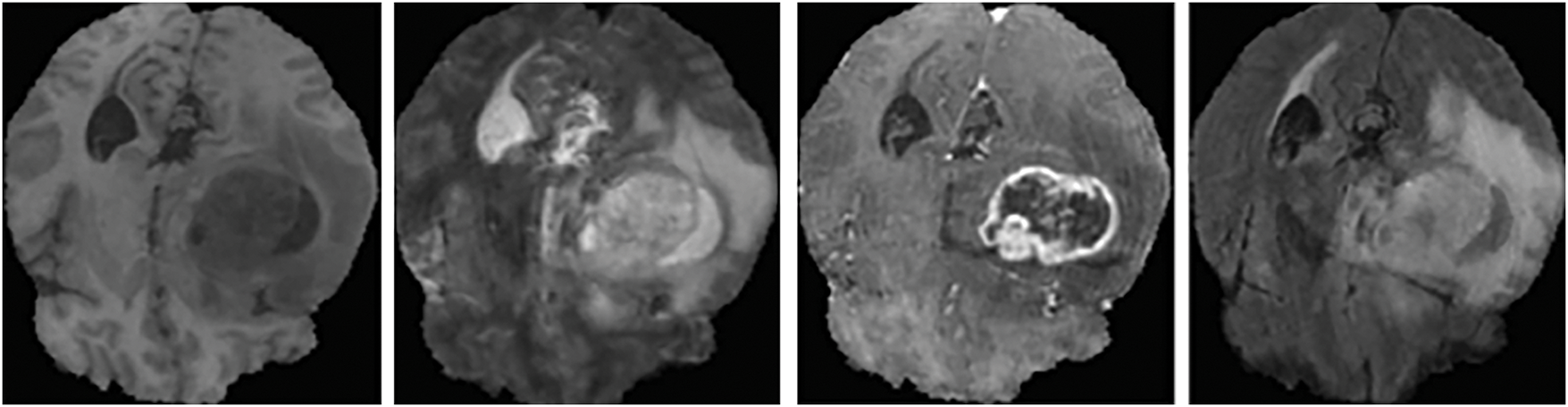
Figure 1: Sample MRI brain scans of Dataset 1

The Dataset 2 (BraTS 2019) is made of 76 lower and 259 higher-grade glioma images. The ground truth in this dataset is manually created using an annotation protocol carried out by neuro-radiologists [39]. The dataset contains MRI brain scans from four modalities: T2, T1, T2-FLAIR and T1-CE. The sample MRI brain scans of Dataset 2 are given in Fig. 2.

Figure 2: Sample MRI brain scans of Dataset 2

Additionally, Dataset 3 (BraTS 2020) comprises of 369 subject data with four modalities which are, Post Contrast T1 weighted (T1CE), T2 weighted (T2), native (T1), and T2 Fluid Attenuated Inversion Recovery (FLAIR) segmented manually, alongside 125 subject data segmented without manual intervention [40]. Furthermore, the sample MRI brain scans of Dataset 3 are illustrated in Fig. 3.

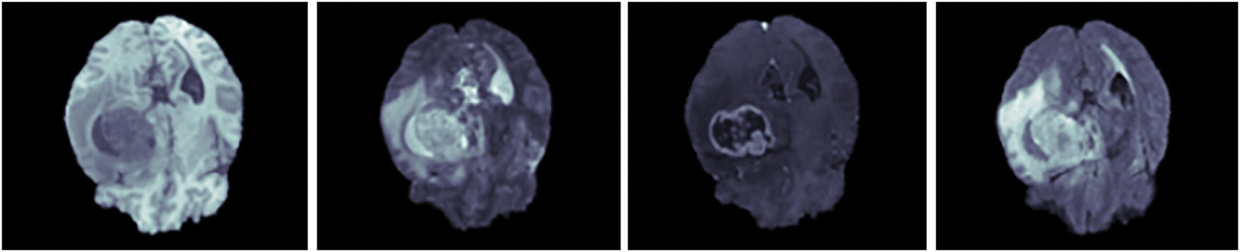
Figure 3: Sample MRI brain scans of Dataset 3

3.2 Brain Lesion Segmentation

After collecting MRI scans, an SNFRC model is proposed for effective BTS, with the MRI scans initially resized to 64×64. Based on existing literature, traditional deep learning models offer improved segmentation performance and greater computational robustness compared to conventional sliding window-based models. However, when dealing with larger input images, the Faster R-CNN model [41] requires significantly more graphics processing unit memory for training. Moreover, traditional Faster R-CNN struggles with fine-grained segmentation, especially in images with complex textures and varying shapes. To overcome these limitations, the proposed SNFRC model incorporates switchable normalization [42], enabling the effective learning and stabilization of multi-scale fine-grained segments. As illustrated in Fig. 4, switchable normalization integrates Layer Normalization (LN), Instance Normalization (IN), and Batch Normalization (BN), allowing dynamic adaptation to varying brain tumor image statistics by learning optimal normalization weights. This results in enhanced generalization, training stability, and better adaptability to heterogeneous tumor textures. In the SNFRC, switchable normalization is critical for accurate multi-scale segmentation, as normalization significantly impacts the detection of fine-grained details across all layers. The model combines a Region Proposal Network (RPN) and a Fast R-CNN detector. The features are first extracted using VGG16, followed by candidate region generation via RPN. These proposals are then aligned with VGG16’s final convolutional layer output and passed through a Region of Interest (ROI) pooling layer to standardize feature dimensions. The resulting features are fed into a fully connected layer to perform the final segmentation, effectively reducing the number of region proposals, improving proposal quality, and enhancing overall detection performance.

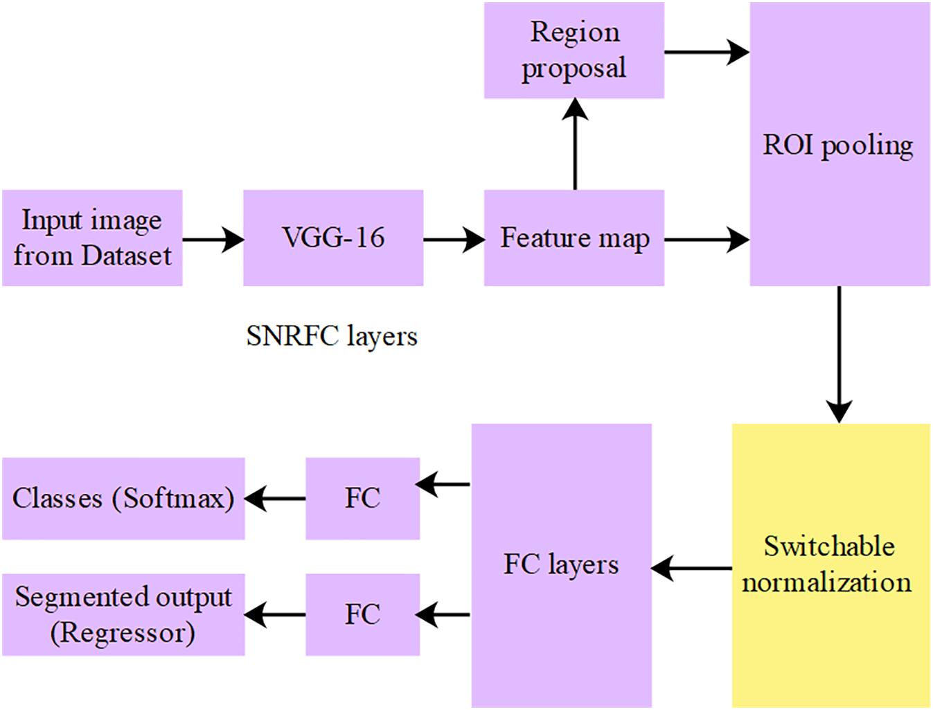
Figure 4: Architecture of SNFRC

The important module in the SNFRC is RPN, which significantly reduces the number of generated region proposals. The RPN identifies pixels using a sliding window applied over the feature representation. Each pixel point lies at the center of a 3×3 convolutional kernel in the sliding window. A receptive region is employed to map the pixel to the image, and this pixel serves as the midpoint for generating nine rectangular regions with three scales (1282,2562,5122) and three aspect ratios (1:3,1:2,1:1), referred to as anchors. These anchors address the challenge of detecting multi-scale objects. The feature map contains multiple pixels, with each pixel corresponding to nine anchors, resulting in a large number of anchors overall. As it is impractical to include all anchors in the training process, a subset is selected for training. The classification probability and anchor’s bounding box regression parameters are obtained by generating region proposals through the integration of the input image into the RPN. Subsequently, the region proposal coordinates are computed, and the proposals refined by Non-Maximum Suppression (NMS) yield high-quality potential regions, contributing to the final outcome of the object identification phase.

The loss function is expressed in Eq. (1).

L({pi},{ti})=1Ncls∑iLcls(pi,pi∗)+λ1Nreg∑ipi∗Lreg(ti,ti∗)(1)

where, the anchor’s index is denoted as i, prediction probability is denoted as pi, ground truth label is denoted as pi∗, the vector with four parameterized coordinates of the discovered box are denoted as ti, ground truth box is depicted as ti∗, weighting parameter is λ, and regression loss and classification loss are denoted as Lcls(pi,pi∗) and Lreg(ti,ti∗). Eqs. (2) and (3) express the classification and regression losses.

Lcls(pi,pi∗)=−log[pi∗pi+(1−pi∗)(1−pi)](2)

Lreg(ti,ti∗)=R(ti−ti∗)(3)

where, the L1 function is denoted as R, the regression loss enabled only for positive anchors (pi∗=1) is denoted as pi∗Lreg, and it is inactivated when pi∗=0. The classification and regression layer outputs are denoted as {pi} and {ti}. The conventional batch normalization function is replaced with switchable normalization in segmentation. Additionally, the dice loss function L is used in the proposed model for balancing the prediction correction, and thereby enabling segmentation to stabilize the acquired fine-grained segments in multi-scale data. During model training, a switchable normalization layer S computes mean μS and variance σS2 which is the layer’s input, as specified mathematically in Eqs. (4) and (5).

μS=1|mS|∑(n,c,i,j)=1mSxncij(4)

σS2=1|mS|∑(n,c,i,j)=1mS(xncij−μS)2(5)

where, every batch has m samples, xi denotes the switchable normalization layer’s input, which is the original pixel in 4D input tensor, S∈{IN,LN,BN} is used to differentiate different methods, 4D tensor considers the width, height, number of channels and number of samples (W,H,C,N), and n,c,i and j are the values taken from 1 to N, 1 to C, 1 to H and 1 to W, respectively. This switchable normalization expressed in Eq. (6), offers a balance of learning and enhances the model’s generalization capacity.

x^ncij=γxncij−∑S∈ΩwSμS∑S∈ΩwS′σS2+λ+β(6)

where, x^ncij is a normalized pixel, a group of valuated statistics is denoted as Ω, scale and shift parameters are denoted as γ and β, respectively, and λ is a small constant used to preserve numerical stability, and wS and wS′ are scalar variables denoting significant rations used to weigh the mean and variances. Here, γ is used to differentiate IN, LN and BN methods.

Furthermore, the layer’s inputs are normalized utilizing the previously computed batch statistics ϵ as denoted in Eq. (7). The output of the layer is obtained by performing scale and shift operations as mentioned in Eq. (8).

xi¯=xi−μSσS2+ϵ(7)

yi=γxi¯+β(8)

where, the parameters γ and β are learned during model training along with the original network parameters. As discussed earlier, the dice loss function L is mathematically stated in Eq. (9).

L=Ldice+0.1×LL2+0.1×LKL(9)

where, Ldice denotes a soft-dice-loss function that improves the decoder Ppred’s output to match the ground-truth masks Ptrue, as represented in Eq. (10).

Ldice=1−2×∑Ppred×Ptrue∑Ppred2+∑Ptrue2(10)

where, LL2 represents L2 loss function and LKL specifies KL divergence which is deployed to induce the Gaussian distribution. The L2 loss and KL divergence functions are mathematically stated in Eqs. (11) and (12).

LL2=∑(INpred−INinput)2(11)

LKL=1N∑μ2+σ2−logσ2−1(12)

where, N denotes the number of image pixels μ2 and σ2 respectively represent mean and variance.

The multi-scale feature maps from VGG16 are aggregated and passed through switchable normalization layers before being fed to the RPN. The regions generated by the RPN are refined through RoI pooling and subsequently forwarded to the tumor-type-specific classifiers and bounding box regressors. The feature representations are stabilized across stages by switchable normalization, which integrates Batch Normalization (BN), Instance Normalization (IN), and Layer Normalization (LN), and is continuously regulated throughout the training process. The feature mapping is illustrated in Fig. 5, along with the corresponding spatial dimensions and normalization operations. At each stage, the depiction of features is enhanced by switchable normalization, which adaptively balances local and global context.

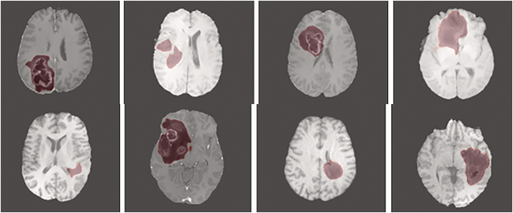
Figure 5: Output image of the proposed model

4  Experimental Results

The proposed segmentation model is executed on Python 3.7 software environment, implemented on a system with 4-TB hard drive, 128-GB random access memory, windows 11 (64-bit) operating system, and Intel i7 12th generation processor. The training of SNFRC is carried out using NVIDIA RTX 2090Ti GPUs, enabling convergence within a reasonable timeframe in accordance with modern deep learning practices in the medical imaging field. Although the computational requirements are higher compared to simpler architectures, this is justified by the improved segmentation performance and enhanced generalizability. Additionally, SNFRC maintains efficient inference speeds, supporting real-time deployment once training is complete. The libraries named TensorFlow, Keras, Numpy, and OpenCV are used to investigate the proposed model’s efficacy. In the acquired datasets, tumor structures are categorized into three sub-regions, namely, Whole-Tumors (WTs) regions, Enhancing Tumors (ETs) regions, and Tumor-Cores (TCs) regions. The ET regions contain label 4, the WT regions exclude ‘edema’ region and comprise the labels 1, 3 and 4, and the TC regions consist of four sub-tumoral classes, such as labels 1, 2, 3, and 4. For each dataset, the training, testing, and validation sets are divided in a 70%, 15%, and 15% ratio, respectively. In this manuscript, the model’s effectiveness is evaluated using the following performance metrics: Hausdorff Distance (HD), recall, F1-measure, Dice Similarity Coefficient (DSC), accuracy, and precision. In brain tumor segmentation (BTS), HD, DSC, Intersection over Union (IoU), and volume similarity are the primary evaluation measures used to validate the efficacy of the segmentation model. The DSC quantifies the overlap between the actual labeled area and the predicted lesion area, and is mathematically defined in Eq. (13). HD is a mathematical metric used to measure the dissimilarity between two sets of points (T and P) in a metric space, as represented in Eq. (14). In segmentation tasks, the correctness of each sample’s identification is related not only to classification but also to localization. Localization accuracy is assessed using IoU, as defined in Eq. (15). Additionally, the overlap among segmented regions is evaluated using volume similarity, expressed in Eq. (16).

DSC=2∗|T∩P||T|+|P|(13)

HD(T,P)=max{supt∈Tinfp∈Pd(t,p),supp∈Pinft∈Td(t,p)}(14)

IoU=P⋂GP⋃G(15)

VolumeSimilarity=1−P−GP+G(16)

where, inf indicates infimum, sup represents supremum, P represents predicted lesion region, T denotes ground truth region, tandp represents the points on the surface P and T. The term d(t,p) estimates the distance between points t and p. In addition, recall assesses the capability of the proposed segmentation model to correctly identify tumor regions from the reference or ground-truth segmentation. Accuracy is also a critical performance measure in BTS and is defined as the proportion of correctly detected observations to the total number of observations. The evaluation measures: recall and accuracy are represented in Eqs. (17) and (18). In these equations, TP indicates the pixels segmented as a tumor region, TN refers to the pixels correctly segmented as background, FP denotes background pixels incorrectly segmented as tumor regions, and FN represents positive pixels incorrectly segmented as background regions.

Recall=TPTP+FN(17)

Accuracy=TP+TNTP+TN+FP+FN(18)

Additionally, precision is defined as the ratio of true positive (TP) predictions to the total number of positive predictions made by the proposed segmentation model. Furthermore, the F1-measure is the harmonic mean of recall and precision. The formulas used to calculate precision and the F1-measure are numerically represented in Eqs. (19) and (20).

Precision=TPTP+FP(19)

F1−measure=2TP2TP+FP+FN(20)

4.1 Performance Evaluation

In this context, the proposed segmentation model is analyzed on three online BraTS datasets. On viewing Table 1, it is seen that the proposed segmentation model achieves impressive outcomes compared to the conventional models: CNN, DenseNet and Faster R-CNN. A graphical comparison of the existing and the proposed model is presented in Figs. 6–8 for all three datasets. This SNFRC model achieves F1-measure of 99.82%, recall of 99.63%, precision of 99.57%, and accuracy of 99.41% on Dataset 1, whereas the comparative models, CNN, DenseNet and Faster R-CNN attain a limited performance in comparison to the SNFRC. The end to end training and efficient region proposal generation of SNFRC helps the model in performing an effective segmentation. The switchable normalization included in the SNFRC helps adapt to normalization for managing changes in brain tumor images, enhancing tumor segmentation with diverse and complex characteristics. Here, the proposed model achieves a higher segmentation performance on a smaller training set as it replicates the feature maps of down sampling which is then integrated with an up-sampling convolutional process for extracting the rich image pixel context information. Similarly, the proposed segmentation model obtains an f1-measure of 97.86%, recall of 98%, precision of 97.63%, and accuracy of 98.12% on Dataset 2. Additionally, on Dataset 3, the model achieves an F1-measure of 96.74%, recall of 96.86%, precision of 96.56%, and accuracy of 96.71%. These numerical results are superior to those of the conventional models.

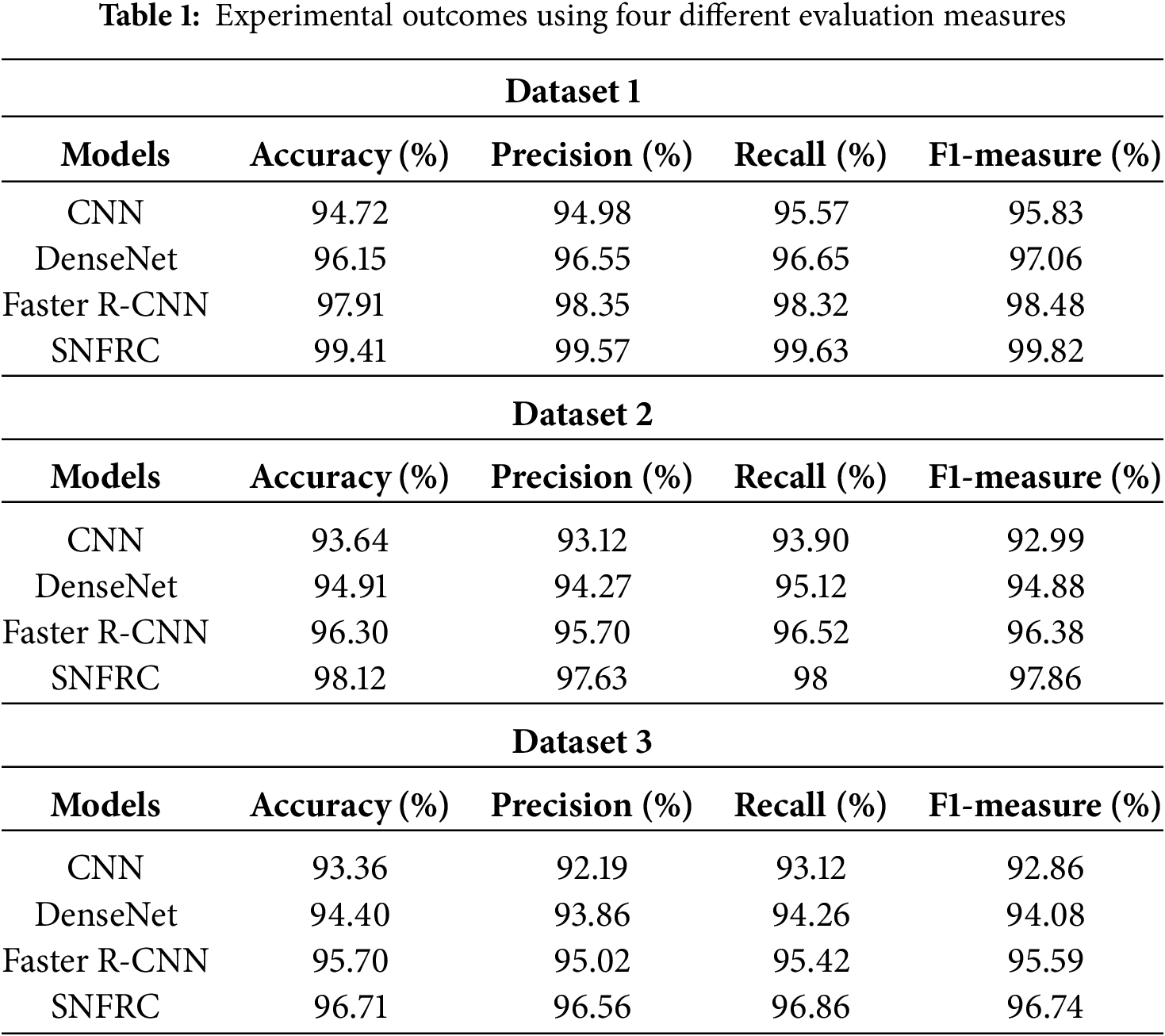
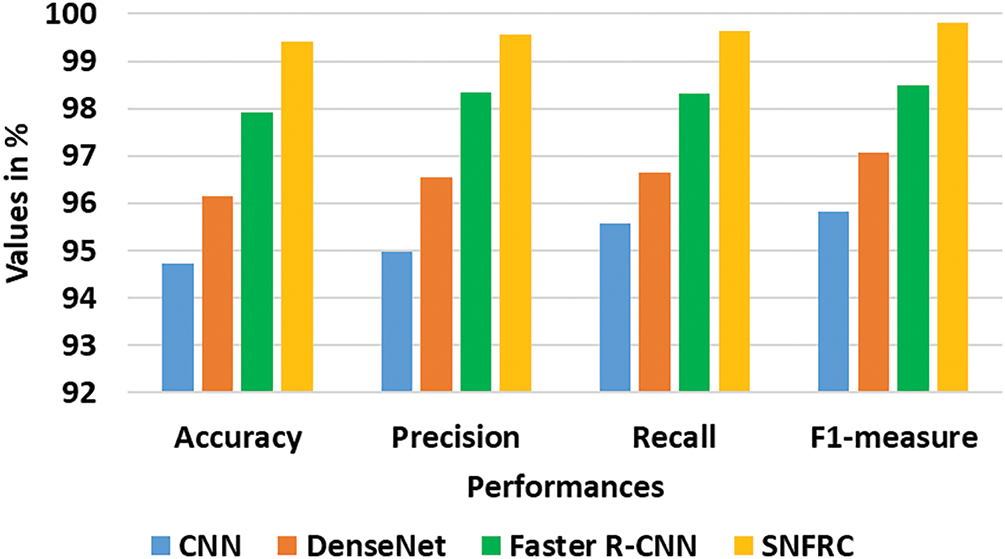
Figure 6: Achieved results of the existing and proposed model on the Dataset 1

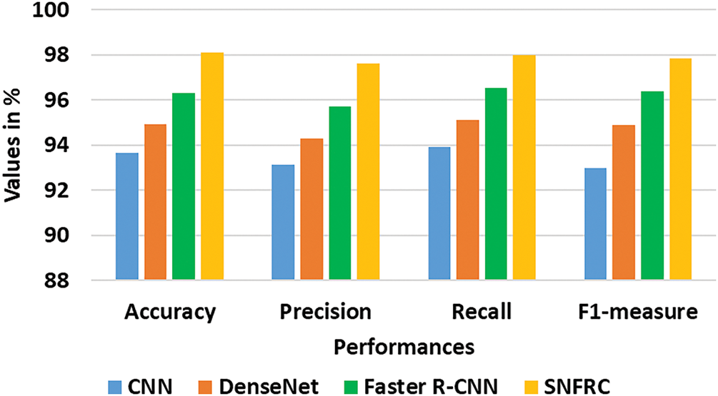
Figure 7: Achieved results of the existing and proposed model on the Dataset 2

Figure 8: Achieved results of the existing and proposed model on the Dataset 3

On the other hand, the overfitting issue in deep learning approaches trained on limited datasets, particularly in medical imaging where annotated data is often scarce, is a well-recognized challenge. In this research, the SNFRC addresses this issue through several strategies: switchable normalization enhances training stability and mitigates covariate shift across feature scales, while edge priors are introduced to promote spatial consistency. These strategies contribute to reliable generalization across the BraTS 2018, 2019, and 2020 datasets, as demonstrated by the model’s performance. Furthermore, the SNFRC is trained on the BraTS 2018 dataset and tested on the BraTS 2019 and BraTS 2020 datasets to evaluate the overfitting risk. This analysis yields accuracies of 97.57% and 94.93% when testing with the BraTS 2019 and BraTS 2020 datasets, respectively.

Fig. 9 shows the performance analysis of accuracy and loss curves for Datasets 1, 2 and 3, respectively used in this research. The accuracy curves validate steady increase throughout the training process and stabilizing at high values which is near to convergence, thus representing that the model efficiently learns the underlying patterns of the respective datasets. Especially, marginal gaps among the training and validation curves prove that the proposed SNFRC model does not experience the overfitting issue. Similarly, the corresponding loss curves display a stable decrease, further confirming the robustness and stability of the training. The stated segmentation accuracies such as 99.41%, 98.12%, and 96.71% are validated by these accuracy and loss curves, providing robust experimental evidence of the model’s effectiveness over various data distributions.

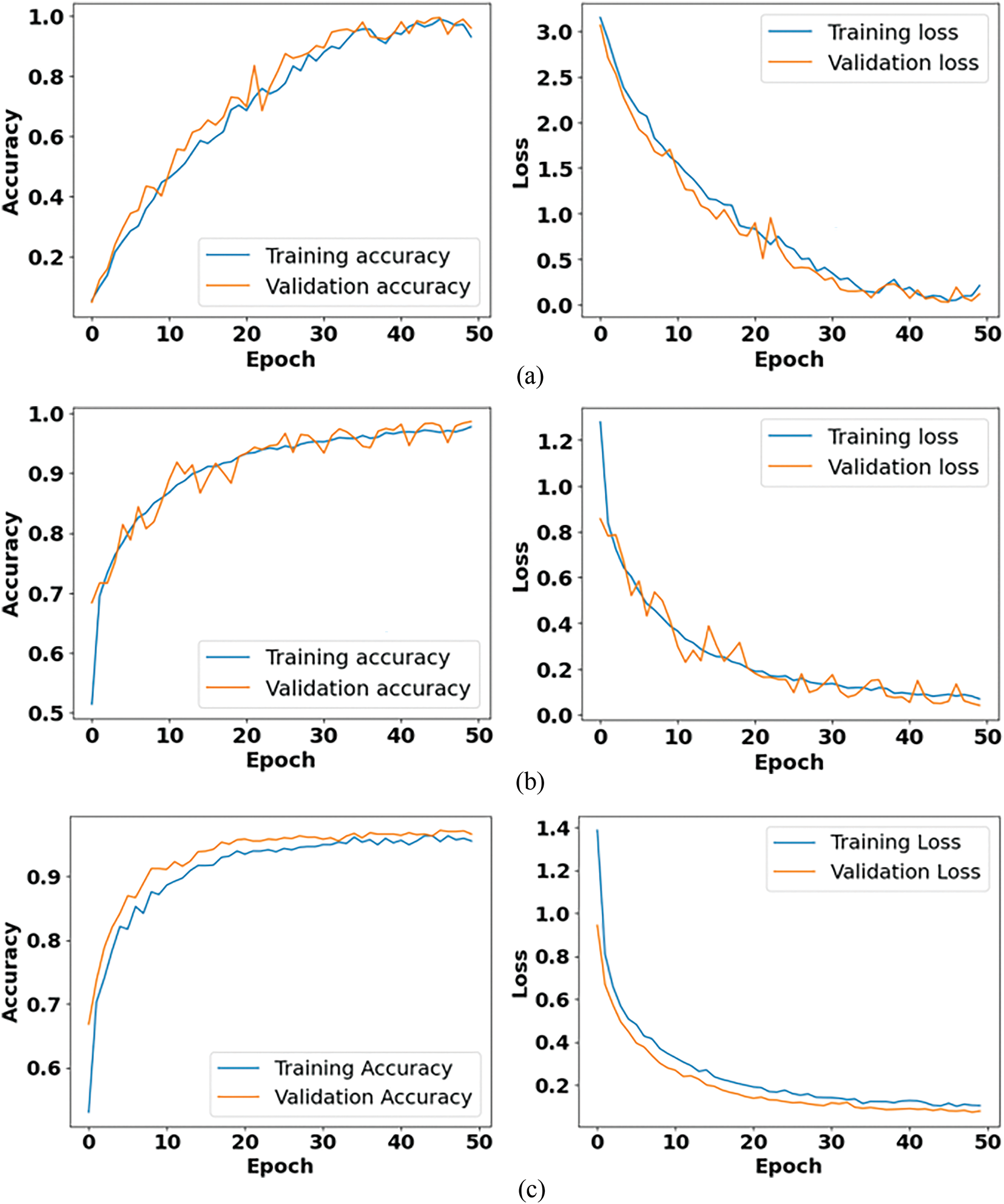
Figure 9: Performance analysis of accuracy and loss curves for (a) Dataset 1, (b) Dataset 2, (c) Dataset 3

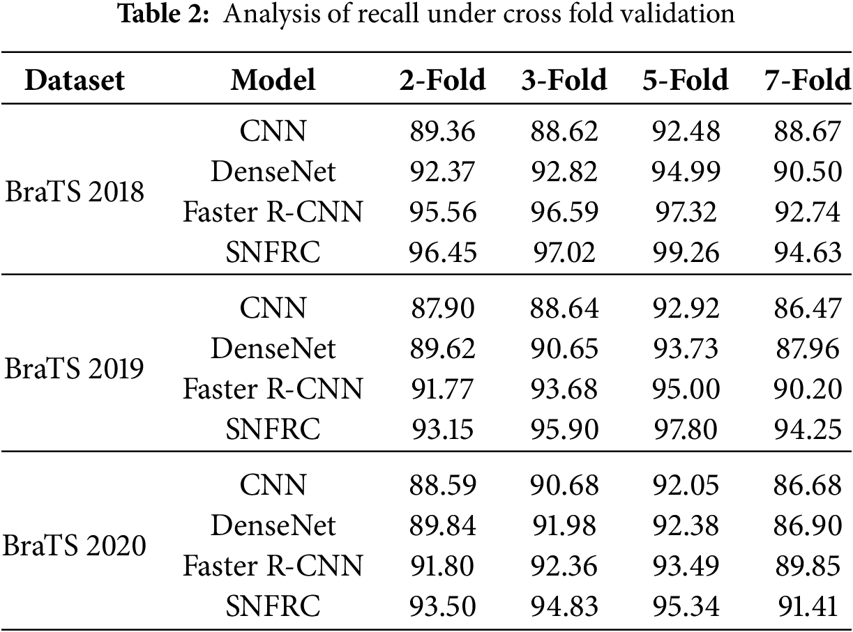
Furthermore, Cross-fold validation is performed, as shown in Table 2, for different fold configurations, including 2-Fold, 3-Fold, 5-Fold, and 7-Fold. Recall is specifically emphasized, as it measures the model’s ability to accurately identify tumor regions, which is crucial for effective tumor segmentation. The SNFRC consistently achieves higher recall across all datasets and fold configurations, demonstrating its superior capacity for brain tumor segmentation (BTS). Even with smaller training splits (e.g., 7-fold), the SNFRC maintains high recall, illustrating its robustness in reliably identifying tumor regions. Larger training sets allow the SNFRC to capture more appropriate tumor features, further enhancing its performance.

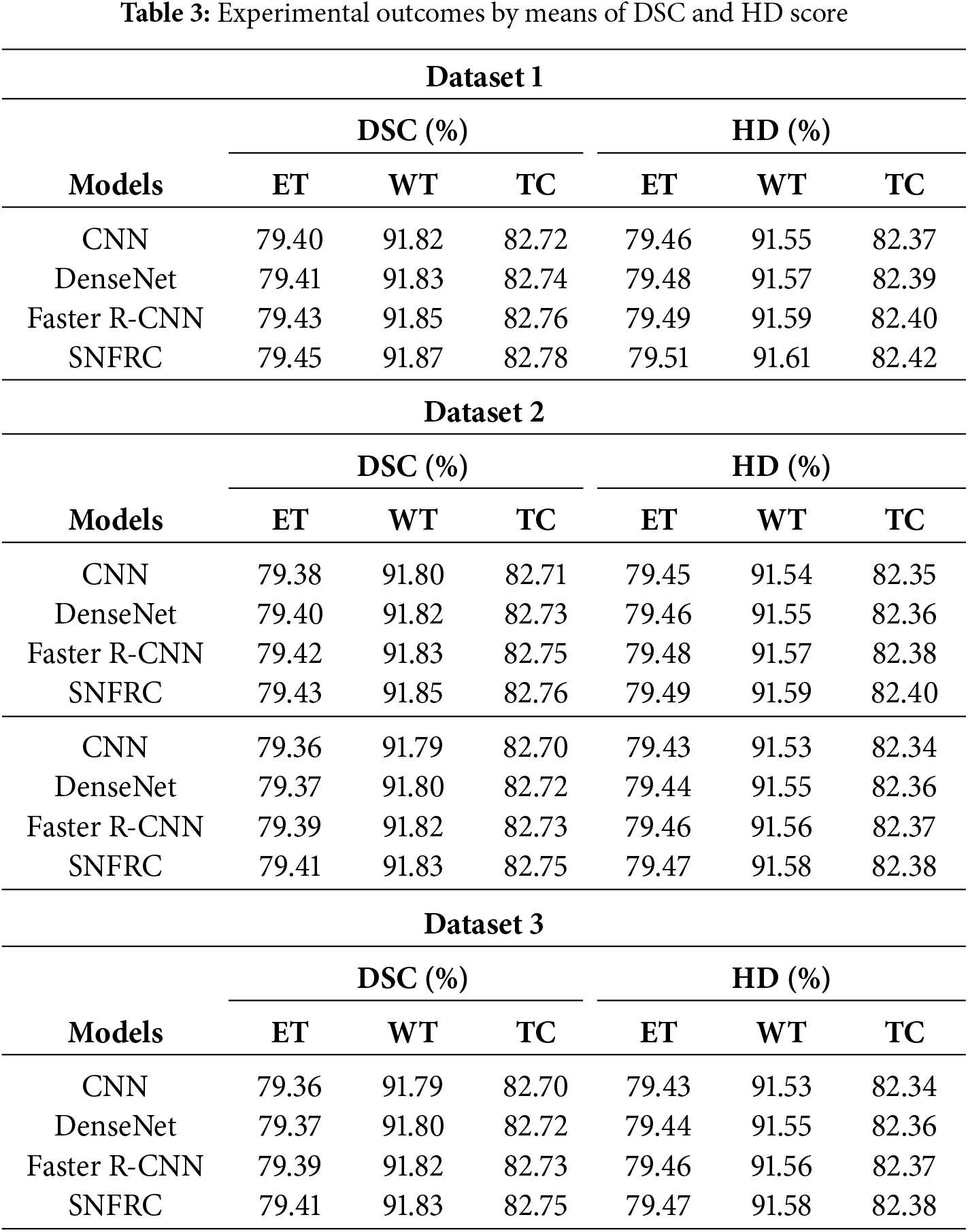
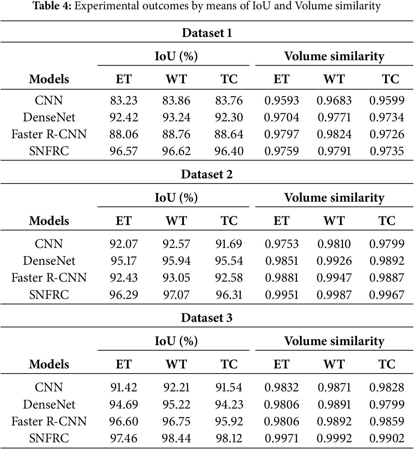
In Tables 3 and 4, the proposed segmentation model’s effectiveness is validated on three online datasets namely, DSC, HD, IoT and volume similarity. From Tables 3 and 4, it is evident that the proposed SNFRC model attains higher segmentation results compared to the CNN, DenseNet and Faster R-CNN on three tumor types (ET, WT, and TC) in terms of DSC, HD, IoT and volume similarity. For example, the proposed SNFRC model obtains a mean DSC of 84.70%, 84.68%, and 84.66%, correspondingly on the Datasets 1, 2, and 3, proving superior to the existing models. The post-processing performed by SNFRC involves applying Non-Maximum Suppression (NMS) after the segmentation layers to eliminate duplicate segmentations while generating the final segmented output.

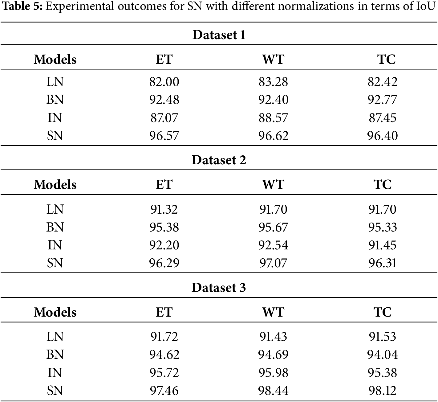
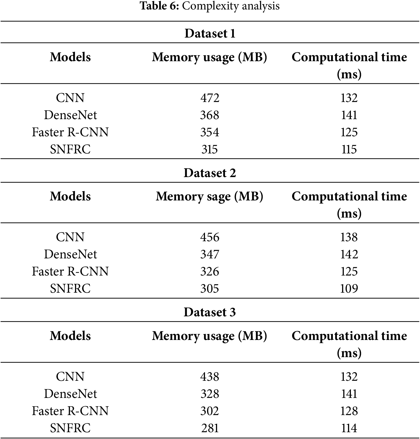
Next, the effectiveness of Switchable Normalization (SN) is analyzed in comparison with other normalization functions such as Layer Normalization (LN), Batch Normalization (BN), and Instance Normalization (IN). Table 5 presents a comparison of SN with these different normalizations using Intersection over Union (IoU), demonstrating that SN outperforms LN, BN, and IN. The complexity analysis in terms of memory usage and computational time required to segment a single image is provided in Table 6. This analysis is specifically conducted due to the increased network depth, which enhances feature differentiation and accuracy. SN offers superior segmentation performance because it adapts to normalization, effectively managing variations in brain tumor images. As a result, SN improves tumor segmentation for images with diverse and complex characteristics. Moreover, the complexity of the SNFRC is lower than that of other approaches such as CNN, DenseNet, and Faster R-CNN. Despite incorporating the additional Switchable Normalization component, the complexity analysis shows that the SNFRC utilizes less computational time and memory than the other approaches. This improved performance is attributed to the optimized normalization and region proposal approach, which minimizes redundant calculations.

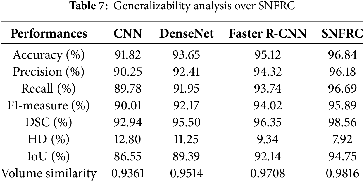
4.2 Analysis on Generalizability

In this section, the generalizability of the proposed SNFRC is evaluated using the Br35H dataset [43]. This dataset consists of 3000 images, including 1500 tumor and 1500 non-tumor images. The results presented in Table 7 indicate that SNFRC generalizes effectively on the Br35H dataset. Specifically, SNFRC achieves high accuracy (96.84%) and recall (95.68%), reflecting improved segmentation quality and boundary precision. The consistent performance of SNFRC highlights the effectiveness of switchable normalization in adapting to varying data distributions.

4.3 Comparative Analysis

An evaluation between the proposed model and comparative models is given in Tables 8 and 9. Zeineldin et al. [16] presented a DeepSeg model for BTS in MRI brain images. The DeepSeg model attains a significant segmentation performance on Dataset 2 in terms of the DSC and HD score. The DeepSeg model obtains 84% of DSC and 9.8% of HD score on the Dataset 2. Zhang et al. [28] introduced an attention gate ResU-Net model for automatic MRI based BTS. This model obtained 87.20%, 77.20%, and 80.80% of DSC for three individual brain tumor types on the Dataset 1. Correspondingly, this model achieved 87%, 70.90%, and 77.70% of DSC value for individual brain tumor types on the Dataset 2.

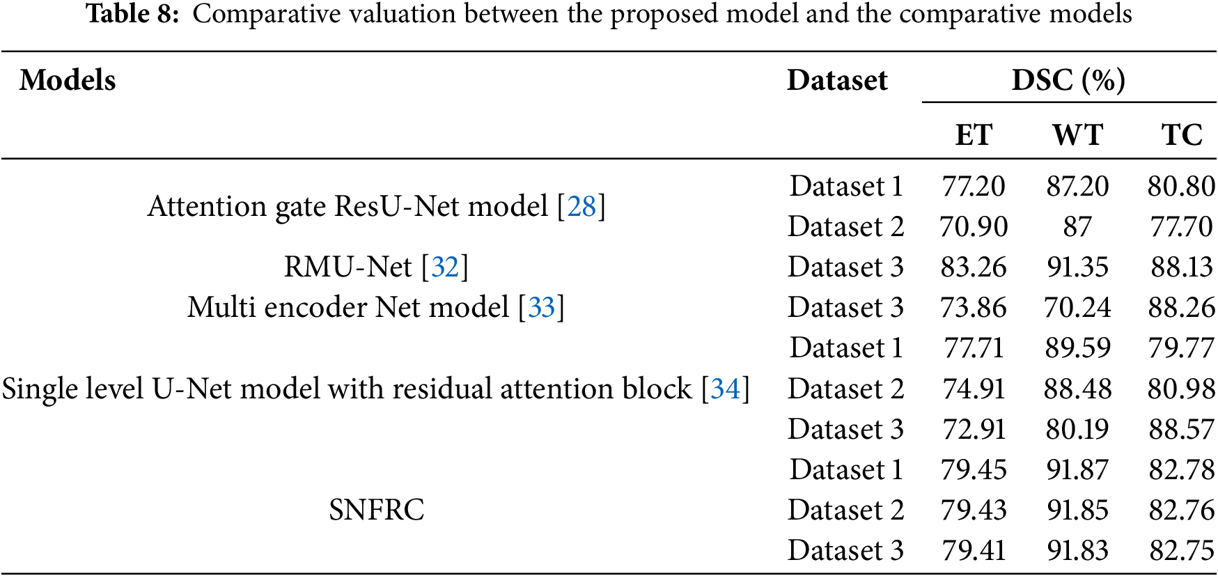
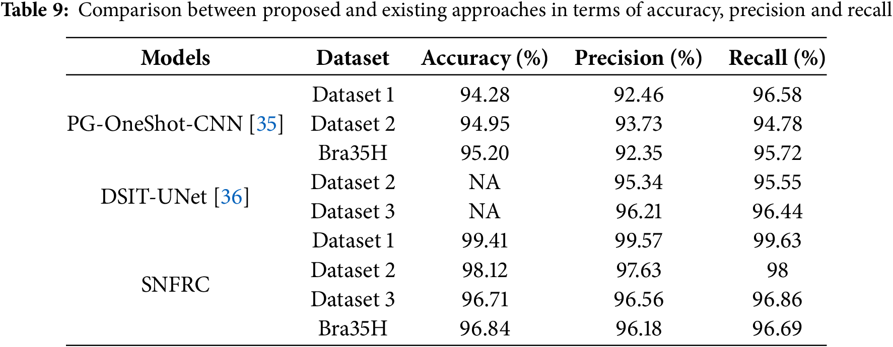
Additionally, Saeed et al. [32] developed RMU-Net for brain tumor segmentation (BTS), which achieved DSC values of 91.35%, 83.26%, and 88.13% on Dataset 3. Similarly, Zhang et al. [33] proposed a multi-encoder network for effective BTS, and extensive experimental analysis showed that this model achieved DSC values of 70.24%, 73.86%, and 88.26% on Dataset 3. Furthermore, Akbar et al. [34] introduced a single-level U-Net model incorporating a residual attention block for improved BTS in MRI brain images. This model achieved DSC values of 89.59%, 77.71%, and 79.77% on Dataset 1 for WT, ET, and TC tumor types, respectively. On Dataset 2, the same model achieved DSC values of 88.48%, 74.91%, and 80.98%, and 88.57%, 72.91%, and 80.19% on Dataset 3. Finally, studies by Ali et al. [35] and Al Hasan et al. [36] are used to compare the proposed SNFRC in terms of accuracy, precision, and recall. This comparative analysis demonstrates that SNFRC consistently outperforms the existing approaches across all evaluation metrics.

The SNFRC employs switchable normalization to dynamically adapt to varying feature distributions across layers, enhancing its ability to generalize across distinct tumor morphologies. This model is further integrated with morphological gradient enhancement and multiscale region proposal mechanisms, which contribute to improved segmentation outcomes for WT, ET, and TC regions. These tumor subtypes exhibit varied structural and textural characteristics. For instance, ET often presents sharp boundary enhancements, while WT is typically associated with diffuse edema, presenting distinct segmentation challenges. However, the improvement is not consistently significant across all cases. Specifically, the DSC for the ET class in Dataset 3 is lower than that achieved by RMU-Net. The recurrent multiscale architecture of RMU-Net is particularly effective in capturing localized patterns within irregular tumor regions such as ET. Nonetheless, SNFRC demonstrates superior overall performance compared to the other existing approaches.

4.4 Discussion

In comparison to the previous models (Attention Gate ResU-Net [28], RMU-Net [32], Multi-Encoder Net [33], and Single-Level U-Net with Residual Attention Block [34]), the proposed model achieves higher BTS performance across Datasets 1, 2, and 3. As discussed in earlier sections, the SNFRC consistently delivers superior BTS results on all three online datasets. However, the reduction in accuracy from Dataset 1 (99.41%) to Dataset 3 (96.71%) highlights the impact of domain shifts caused by temporal and institutional variability, including differences in MRI protocols, patient demographics, and scanner hardware. These factors reflect real-world clinical heterogeneity and present ongoing challenges for model generalization. Switchable normalization combines the strengths of instance normalization, layer normalization, and batch normalization, with the ability to switch among these normalization modes, enabling SNFRC to adapt to the specific characteristics of the image data. In this context, the adaptability of switchable normalization leads to improved feature representation within the traditional Faster R-CNN architecture. Therefore, the proposed model is robust and well-suited for accurate brain tumor segmentation, effectively capturing subtle patterns and variations in MRI medical images.

5  Conclusion

This paper proposed SNFRC to enhance the segmentation accuracy and generalization of brain tumor segmentation (BTS) by integrating switchable normalization (SN) into the Faster R-CNN framework. The inclusion of SN enables dynamic adaptation to varying brain tumor image statistics. The extraction of multiscale fine-grained segments contributes to improved generalization, training stability, and adaptability to different tumor textures, particularly in heterogeneous image scenarios. Additionally, the incorporation of the morphological gradient function and Dice loss function enhances tumor pixel segmentation and reduces feature information loss. For experimental analysis, three BraTS datasets are utilized. The proposed segmentation model demonstrates robustness, achieving accuracies of 99.41%, 98.12%, and 96.71% on Datasets 1, 2, and 3, respectively. These numerical results are significant when compared to traditional models such as CNN, DenseNet, and Faster R-CNN, based on evaluation metrics including HD, recall, F1-measure, DSC, accuracy, and precision. The generalization capability of SNFRC is further validated through its effective segmentation performance on the Br35H dataset. This highlights the model’s potential, although certain challenges remain. Future work may focus on integrating an appropriate classification model to classify medical image subtypes. To address the issue of overfitting in low-data scenarios, future research can explore self-supervised pretraining and uncertainty-aware learning to enhance robustness. Furthermore, the model’s performance under real-world imaging artifacts can be investigated using multi-center data and noise-augmented conditions.

Acknowledgement: The authors express gratitude to the anonymous reviewers for their valuable insights and feedback on earlier versions of this paper.

Funding Statement: This research was supported by the Basic Science Research Program through the National Research Foundation of Korea (NRF) funded by the Ministry of Science and ICT (NRF-2022R1A2C2012243).

Author Contributions: The paper investigation, resources, data curation, writing—original draft preparation, writing—review and editing, and visualization were conducted by Rachana Poongodan and Dayanand Lal Narayan. The paper conceptualization and software were conducted by Hirald Dwaraka Praveena and Deepika Gadakatte Lokeshwarappa. The validation and formal analysis, methodology, supervision, project administration, and funding acquisition of the version to be published were conducted by Dae-Ki Kang. All authors reviewed the results and approved the final version of the manuscript.

Availability of Data and Materials: The datasets generated during and/or analyzed during the current study are available in the [BraTs] repositories. Dataset 1: https://www.kaggle.com/datasets/sanglequang/brats2018 (accessed on 01 June 2025).Dataset 2: https://github.com/woodywff/brats_2019 (accessed on 01 June 2025). Dataset 3: https://www.kaggle.com/datasets/awsaf49/brats2020-training-data (accessed on 01 June 2025).

Ethics Approval: Not applicable.

Conflicts of Interest: The authors declare no conflicts of interest to report regarding the present study.

References

1. Zhou Z, He Z, Jia Y. AFPNet: a 3D fully convolutional neural network with atrous-convolution feature pyramid for brain tumor segmentation via MRI images. Neurocomputing. 2020;402(11):235–44. doi:10.1016/j.neucom.2020.03.097. [Google Scholar] [CrossRef]

2. Narmatha C, Eljack SM, Tuka AARM, Manimurugan S, Mustafa M. A hybrid fuzzy brain-storm optimization algorithm for the classification of brain tumor MRI images. J Ambient Intell Humaniz Comput. 2020;1–9. doi:10.1007/s12652-020-02470-5. [Google Scholar] [CrossRef]

3. Abdelaziz Ismael SA, Mohammed A, Hefny H. An enhanced deep learning approach for brain cancer MRI images classification using residual networks. Artif Intell Med. 2020;102(6):101779. doi:10.1016/j.artmed.2019.101779. [Google Scholar] [PubMed] [CrossRef]

4. Myronenko A. 3D MRI brain tumor segmentation using autoencoder regularization. In: Crimi A, Bakas S, Kuijf H, Keyvan F, Reyes M, van Walsum T, editors. Brainlesion: glioma, multiple sclerosis, stroke and traumatic brain injuries. Berlin/Heidelberg, Germany: Springer; 2018. p. 311–20. doi:10.1007/978-3-030-11726-9_28. [Google Scholar] [CrossRef]

5. Li H, Li A, Wang M. A novel end-to-end brain tumor segmentation method using improved fully convolutional networks. Comput Biol Med. 2019;108(11):150–60. doi:10.1016/j.compbiomed.2019.03.014. [Google Scholar] [PubMed] [CrossRef]

6. Feng X, Tustison NJ, Patel SH, Meyer CH. Brain tumor segmentation using an ensemble of 3D U-nets and overall survival prediction using radiomic features. Front Comput Neurosci. 2020;14:25. doi:10.3389/fncom.2020.00025. [Google Scholar] [PubMed] [CrossRef]

7. Khan AR, Khan S, Harouni M, Abbasi R, Iqbal S, Mehmood Z. Brain tumor segmentation using K-means clustering and deep learning with synthetic data augmentation for classification. Microsc Res Tech. 2021;84(7):1389–99. doi:10.1002/jemt.23694. [Google Scholar] [PubMed] [CrossRef]

8. Razzak MI, Imran M, Xu G. Efficient brain tumor segmentation with multiscale two-pathway-group conventional neural networks. IEEE J Biomed Health Inform. 2019;23(5):1911–9. doi:10.1109/JBHI.2018.2874033. [Google Scholar] [PubMed] [CrossRef]

9. Thillaikkarasi R, Saravanan S. An enhancement of deep learning algorithm for brain tumor segmentation using kernel based CNN with M-SVM. J Med Syst. 2019;43(4):84. doi:10.1007/s10916-019-1223-7. [Google Scholar] [PubMed] [CrossRef]

10. Daimary D, Bora MB, Amitab K, Kandar D. Brain tumor segmentation from MRI images using hybrid convolutional neural networks. Procedia Comput Sci. 2020;167(6):2419–28. doi:10.1016/j.procs.2020.03.295. [Google Scholar] [CrossRef]

11. Tong J, Zhao Y, Zhang P, Chen L, Jiang L. MRI brain tumor segmentation based on texture features and kernel sparse coding. Biomed Signal Process Control. 2019;47(2):387–92. doi:10.1016/j.bspc.2018.06.001. [Google Scholar] [CrossRef]

12. Ben Naceur M, Akil M, Saouli R, Kachouri R. Fully automatic brain tumor segmentation with deep learning-based selective attention using overlapping patches and multi-class weighted cross-entropy. Med Image Anal. 2020;63(1):101692. doi:10.1016/j.media.2020.101692. [Google Scholar] [PubMed] [CrossRef]

13. Lin WW, Cheng J, Yueh MH, Huang TM, Li T, Wang S, et al. 3D brain tumor segmentation using a two-stage optimal mass transport algorithm. Sci Rep. 2021;11(1):14686. doi:10.1038/s41598-021-94071-1. [Google Scholar] [PubMed] [CrossRef]

14. Rehman MU, Cho S, Kim JH, Chong KT. BU-Net: brain tumor segmentation using modified U-Net architecture. Electronics. 2020;9(12):2203. doi:10.3390/electronics9122203. [Google Scholar] [CrossRef]

15. Wang W, Chen C, Ding M, Yu H, Zha S, Li J. TransBTS: multimodal brain tumor segmentation using transformer. In: Proceedings of 24th International Conference on Medical Image Computing and Computer-Assisted Intervention (MICCAI 2021); 2021 Sep 27–Oct 1; Strasbourg, France. p. 109–19. [Google Scholar]

16. Zeineldin RA, Karar ME, Coburger J, Wirtz CR, Burgert O. DeepSeg: deep neural network framework for automatic brain tumor segmentation using magnetic resonance FLAIR images. Int J Comput Assist Radiol Surg. 2020;15(6):909–20. doi:10.1007/s11548-020-02186-z. [Google Scholar] [PubMed] [CrossRef]

17. Chen S, Ding C, Liu M. Dual-force convolutional neural networks for accurate brain tumor segmentation. Pattern Recognit. 2019;88(suppl_5):90–100. doi:10.1016/j.patcog.2018.11.009. [Google Scholar] [CrossRef]

18. Havaei M, Davy A, Warde-Farley D, Biard A, Courville A, Bengio Y, et al. Brain tumor segmentation with deep neural networks. Med Image Anal. 2017;35(4):18–31. doi:10.1016/j.media.2016.05.004. [Google Scholar] [PubMed] [CrossRef]

19. Pereira S, Pinto A, Alves V, Silva CA. Brain tumor segmentation using convolutional neural networks in MRI images. IEEE Trans Med Imag. 2016;35(5):1240–51. doi:10.1109/TMI.2016.2538465. [Google Scholar] [PubMed] [CrossRef]

20. Abdel-Maksoud E, Elmogy M, Al-Awadi R. Brain tumor segmentation based on a hybrid clustering technique. Egypt Inform J. 2015;16(1):71–81. doi:10.1016/j.eij.2015.01.003. [Google Scholar] [CrossRef]

21. Zhao X, Wu Y, Song G, Li Z, Zhang Y, Fan Y. A deep learning model integrating FCNNs and CRFs for brain tumor segmentation. Med Image Anal. 2018;43:98–111. doi:10.1016/j.media.2017.10.002. [Google Scholar] [PubMed] [CrossRef]

22. Zhang D, Huang G, Zhang Q, Han J, Han J, Yu Y. Cross-modality deep feature learning for brain tumor segmentation. Pattern Recognit. 2021;110(11):107562. doi:10.1016/j.patcog.2020.107562. [Google Scholar] [CrossRef]

23. Alqazzaz S, Sun X, Yang X, Nokes L. Automated brain tumor segmentation on multi-modal MR image using SegNet. Comput Vis Medium. 2019;5(2):209–19. doi:10.1007/s41095-019-0139-y. [Google Scholar] [CrossRef]

24. Zhou X, Li X, Hu K, Zhang Y, Chen Z, Gao X. ERV-Net: an efficient 3D residual neural network for brain tumor segmentation. Expert Syst Appl. 2021;170(8):114566. doi:10.1016/j.eswa.2021.114566. [Google Scholar] [CrossRef]

25. Nema S, Dudhane A, Murala S, Naidu S. RescueNet: an unpaired GAN for brain tumor segmentation. Biomed Signal Process Control. 2020;55:101641. doi:10.1016/j.bspc.2019.101641. [Google Scholar] [CrossRef]

26. Iqbal S, Ghani MU, Saba T, Rehman A. Brain tumor segmentation in multi-spectral MRI using convolutional neural networks (CNN). Microsc Res Tech. 2018;81(4):419–27. doi:10.1002/jemt.22994. [Google Scholar] [PubMed] [CrossRef]

27. Hu K, Gan Q, Zhang Y, Deng S, Xiao F, Huang W, et al. Brain tumor segmentation using multi-cascaded convolutional neural networks and conditional random field. IEEE Access. 2019;7:92615–29. doi:10.1109/ACCESS.2019.2927433. [Google Scholar] [CrossRef]

28. Zhang J, Jiang Z, Dong J, Hou Y, Liu B. Attention gate ResU-net for automatic MRI brain tumor segmentation. IEEE Access. 2020;8:58533–45. doi:10.1109/ACCESS.2020.2983075. [Google Scholar] [CrossRef]

29. Aboelenein NM, Piao S, Koubaa A, Noor A, Afifi A. HTTU-Net: hybrid two track U-Net for automatic brain tumor segmentation. IEEE Access. 2020;8:101406–15. doi:10.1109/access.2020.2998601. [Google Scholar] [CrossRef]

30. Zhang C, Shen X, Cheng H, Qian Q. Brain tumor segmentation based on hybrid clustering and morphological operations. Int J Biomed Imaging. 2019;2019(3):7305832–11. doi:10.1155/2019/7305832. [Google Scholar] [PubMed] [CrossRef]

31. Ding Y, Gong L, Zhang M, Li C, Qin Z. A multi-path adaptive fusion network for multimodal brain tumor segmentation. Neurocomputing. 2020;412(1):19–30. doi:10.1016/j.neucom.2020.06.078. [Google Scholar] [CrossRef]

32. Saeed MU, Ali G, Bin W, Almotiri SH, AlGhamdi MA, Ali Nagra A, et al. RMU-Net: a novel residual mobile U-Net model for brain tumor segmentation from MR images. Electronics. 2021;10(16):1962. doi:10.3390/electronics10161962. [Google Scholar] [CrossRef]

33. Zhang W, Yang G, Huang H, Yang W, Xu X, Liu Y, et al. ME-Net: multi-encoder net framework for brain tumor segmentation. Int J Imag Syst Technol. 2021;31(4):1834–48. doi:10.1002/ima.22571. [Google Scholar] [CrossRef]

34. Akbar AS, Fatichah C, Suciati N. Single level UNet3D with multipath residual attention block for brain tumor segmentation. J King Saud Univ Comput Inf Sci. 2022;34(6):3247–58. doi:10.1016/j.jksuci.2022.03.022. [Google Scholar] [CrossRef]

35. Ali A, Wang Y, Shi X. Segmentation and identification of brain tumour in MRI images using PG-OneShot learning CNN model. Multimed Tools Appl. 2024;83(34):81361–82. doi:10.1007/s11042-024-18596-z. [Google Scholar] [CrossRef]

36. Al Hasan S, Mahim SM, Hossen ME, Hasan MO, Islam MK, Livreri P, et al. DSIT UNet a dual stream iterative transformer based UNet architecture for segmenting brain tumors from FLAIR MRI images. Sci Rep. 2025;15(1):13815. doi:10.1038/s41598-025-98464-4. [Google Scholar] [PubMed] [CrossRef]

37. Rahman MA, Masum MI, Hasib KM, Mridha MF, Alfarhood S, Safran M, et al. GliomaCNN: an effective lightweight CNN model in assessment of classifying brain tumor from magnetic resonance images using explainable AI. Comput Model Eng Sci. 2024;140(3):2425–48. doi:10.32604/cmes.2024.050760. [Google Scholar] [CrossRef]

38. Lin M, Momin S, Lei Y, Wang H, Curran WJ, Liu T, et al. Fully automated segmentation of brain tumor from multiparametric MRI using 3D context deep supervised U-Net. Med Phys. 2021;48(8):4365–74. doi:10.1002/mp.15032. [Google Scholar] [PubMed] [CrossRef]

39. Sharif MI, Li JP, Amin J, Sharif A. An improved framework for brain tumor analysis using MRI based on YOLOv2 and convolutional neural network. Complex Intell Syst. 2021;7(4):2023–36. doi:10.1007/s40747-021-00310-3. [Google Scholar] [CrossRef]

40. Rehman A, Khan MA, Saba T, Mehmood Z, Tariq U, Ayesha N. Microscopic brain tumor detection and classification using 3D CNN and feature selection architecture. Microsc Res Tech. 2021;84(1):133–49. doi:10.1002/jemt.23597. [Google Scholar] [PubMed] [CrossRef]

41. Tang W, Zou D, Yang S, Shi J, Dan J, Song G. A two-stage approach for automatic liver segmentation with Faster R-CNN and DeepLab. Neural Comput Appl. 2020;32(11):6769–78. doi:10.1007/s00521-019-04700-0. [Google Scholar] [CrossRef]

42. Luo P, Zhang R, Ren J, Peng Z, Li J. Switchable normalization for learning-to-normalize deep representation. IEEE Trans Pattern Anal Mach Intell. 2021;43(2):712–28. doi:10.1109/TPAMI.2019.2932062. [Google Scholar] [PubMed] [CrossRef]

43. Br35H :: brain tumor detection. 2020 [cited 2025 Jan 1]. Available from: https://www.kaggle.com/datasets/ahmedhamada0/brain-tumor-detection. [Google Scholar]