The Identification of Influential Users Based on Semi-Supervised Contrastive Learning

1  Introduction

With the rise of social networking platforms such as Twitter, Facebook, and Weibo, a specific group of users, known as influential users, has emerged. These users’ behaviors can significantly affect others within the network. Accurately identifying influential users can effectively reduce the costs associated with commercial promotion [1] and public opinion management [2]. In different networks, influential users manifest in various forms, such as celebrities or domain experts. In this paper, no distinction is made among these influential users. Instead, influential users are defined herein as users in social networks who are recognized by other users and possess strong information dissemination capabilities.

Some studies [3–5] have employed relationship network-based approaches to identify influential users. These methods utilize social relationship graphs derived from user interactions to detect influential users, treating them as key nodes within complex networks. The identification is achieved by exploiting the structural differences between influential users and ordinary users. Although such methods exhibit high computational efficiency and require little labeled data, their reliance solely on structural information from the relationship network limits both their accuracy and coverage.

Other studies [6–8] have adopted user feature-based approaches to identify influential users. These methods extract user features from data such as user attributes and posting behaviors, identifying influential users either by manually defining feature patterns or by training models on large amounts of labeled data to capture the distinctions between known influential users and ordinary users. However, the performance of these approaches heavily depends on the selection of features. Since the raw user features are diverse and many of them are weakly correlated with user influence, extensive feature engineering is often required to achieve satisfactory results.

The aforementioned methods identify influential users based solely on relationship networks or user features, resulting in a relatively superficial characterization of users and leading to low identification accuracy. In recent years, methods based on Graph Neural Networks (GNNs) have been proposed [9–12]. Study [9] achieved better results by introducing an autoencoder to capture diverse and complementary information from multiple perspectives, thereby generating more comprehensive node representations.

However, methods based on GNNs [9–12] have several drawbacks: When applying GNNs to user classification tasks, adjacent users are often assumed to belong to the same category, a premise that underlies most classification scenarios. Under this premise, Graph Convolutional Networks (GCNs) [13] and other GNNs are typically designed to aggregate users’ features in such a way that adjacent users’ features are close to each other. However, in the task of identifying influential users, these users constitute a minority in the entire dataset, and they are more likely to have relationships with other users compared to ordinary users. As a result, most neighbors of influential users are ordinary users. In such cases, the neighborhood similarity characteristic of GNNs may cause influential users and some ordinary users to have similar representations, thereby increasing the difficulty of classification and requiring more training data to achieve accurate results.

To address this issue, we propose using contrastive learning to guide GNNs in extracting user features. Existing research [14–16] has demonstrated that in most cases, influential users differ significantly from ordinary users in terms of centrality indices that reflect user influence. These centrality indices can be directly calculated without labeled data. By leveraging these centrality indices, reasonable positive and negative samples can be provided for contrastive learning. If contrastive learning can obtain more discriminative user features, it can not only improve the accuracy of identification but also reduce the difficulty of training.

Specifically, we propose a semi-supervised contrastive learning method for identifying influential users. The proposed method employs a GCN as an encoder to integrate users’ network structures and user features into node representations. To ensure that the learned representations effectively capture the characteristics of influential users, three node centrality metrics, which reflect user influence, are utilized to construct positive and negative sample pairs. A contrastive learning strategy is applied to minimize the feature distance between users of the same class while maximizing the distance between users of different classes, thereby guiding the encoder to extract more accurate representations of influential users. Subsequently, a small amount of labeled data is used to train an attention mechanism-based user classifier to accomplish the influential user identification task.

The remainder of this paper is organized as follows: Section 2 reviews the related work on influential user identification. Section 3 presents the proposed method and outlines its main steps. Section 4 evaluates the effectiveness of the proposed approach through experiments and analyzes the results. Section 5 discusses the applicability of the proposed method under different scenarios. Section 6 concludes the paper and discusses future research directions.

2  Related Work

Driven by practical application demands, influential user identification has gradually become an increasingly prominent research direction. Existing approaches can be broadly classified into three categories: relationship network-based influential user identification methods, user feature-based methods, and Graph Neural Network (GNN)-based methods.

2.1 Influential User Identification Based on Relationship Networks

Recent research on social networks identifies influential users by evaluating node importance using graph-based metrics. These methods are typically based on centrality measures, such as degree centrality and closeness centrality [3]. For instance, the study in [4] proposed Escape Velocity Centrality (EVC) by drawing an analogy to escape velocity in physics, which integrates multiple centrality measures to differentiate influential users from ordinary users. This metric is characterized by low computational complexity combined with high accuracy, enabling the effective identification of influential nodes within networks. The study in [5] argued that although user influence is correlated with centrality, manually combining centrality measures may only be effective for certain types of networks. To address this, the authors employed a convolutional network to learn users’ local, community, and global features and trained their model on synthetic Barabási–Albert (BA) networks. However, these network-based methods tend to oversimplify user representations, which results in relatively low identification accuracy.

2.2 Influential User Identification Based on User Features

Recent research identifies influential users by modeling differences in user attributes and posting behaviors between them and ordinary users. The study [6] utilized all available profile attributes of users on the Reddit platform and applied association rule mining techniques to identify influential users. It further indicated that, in addition to conventional influence-related factors such as the number of followers, demographic variables, including gender and age, also contribute to the identification of influential users. The study [7] found that influential users who had served as chairs in large online open-source organizations exhibited significant linguistic differences compared to ordinary users. The study employed a psychology-oriented lexicon and logistic regression to identify these influential users. A more recent study [8] extracted textual features from users’ posts using TextCNN and LSTM architectures, concatenated them with user attributes such as lifecycle and geographic location, and applied ensemble learning methods to identify influential users. Such methods rely heavily on complex feature engineering and complete user datasets. However, privacy protection policies in social networks make it difficult to obtain user data, and the complexity of feature engineering significantly hampers their practical applicability.

2.3 Influential User Identification Based on Graph Neural Networks

Recent GNN-based approaches capture the structural and feature-based differences between influential users and ordinary users, thereby generating more comprehensive user representations and achieving improved identification performance. The study [10] proposed a social influence prediction framework, DeepInf, which samples the social network through random walks and utilizes GCN and GAT [14] to learn latent social representations of users, enabling user influence prediction. The study [11] introduced an influence prediction framework, InfGCN, which argued that the importance of relationships varies among users. It determines edge weights by computing node betweenness centrality and concatenating four types of centrality metrics with user features. These combined features were input into GCN to generate node representation vectors, resulting in improved performance. The study [12] suggested that both the importance of users and their relationships variy, and proposed a method to assess individual user reputation and interpersonal trust between users. A network was constructed based on user reputation and interpersonal trust, and GNN was applied to identify influential users. The features of influential users learned by GNNs through neighborhood aggregation mechanisms are often insufficiently discriminative and require a substantial amount of labeled data for training, thereby limiting their practicality.

3  Method

A study [17] has highlighted the extensive applications and significant potential of semi-supervised learning in the graph domain. Inspired by this study, this paper proposes an influential user identification method based on semi-supervised contrastive learning. The framework of the method is shown in Fig. 1. Specifically, it comprises four components: positive and negative sample pair construction, an encoder, contrastive learning, and influential user identification. The proposed method first selects three centrality indices, each closely related to user influence, to represent a node’s individual, community, and global influence. Based on these rankings, positive and negative sample pairs are constructed. Then, a two-layer GCN, followed by a fully connected layer, is employed as an encoder to learn node representations from the graph. Through contrastive learning, the encoder is guided to generate discriminative vectors that accurately represent influential users. Finally, a classifier based on an attention network is fine-tuned using a small amount of labeled data, integrating the three types of vectors to identify influential users. The main steps of the method are as follows:

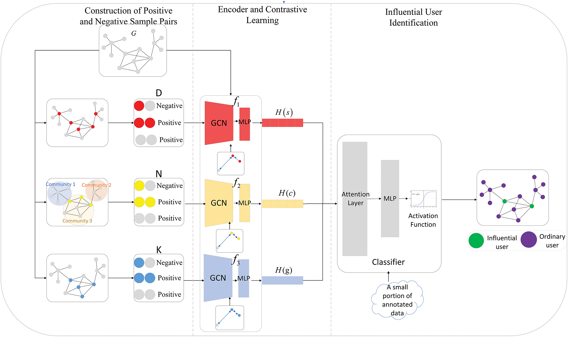
Figure 1: Method flowchart

Step 1: Construction of Positive and Negative Sample Pairs

In the given graph G, calculate the centrality indices D(vi), Ncom(vi), and k−core(vi) for each user vi. Select nodes ranked in the top α%  as the positive class and the remaining nodes as the negative class. Form positive sample pairs with nodes of the same class and negative sample pairs with nodes of different classes, resulting in three sets of positive and negative samples: D, N, and K.

Step 2: User Encoding

In the given graph G, construct three encoders f1, f2, and f3 with identical structures, each consisting of a two-layer GCN followed by a fully connected layer to learn user representation vectors.

Step 3: Contrastive Learning

Using the three sets of positive and negative samples D, N, and K, train the encoders f1, f2, and f3 to obtain three vectors H(s), H(c), and H(g) that reflect user influence.

Step 4: influential User Identification

For the obtained vectors H(s), H(c), and H(g) that reflect user influence, construct a classifier consisting of an attention network and a fully connected layer. Fuse the user vectors obtained from different encoders and identify influential users.

In the following section, we discuss the implementation process in detail

3.1 Construction of Positive and Negative Sample Pairs

Constructing appropriate positive and negative samples is crucial in contrastive learning. During training, inappropriate sample pairs may mislead the model, preventing it from accurately extracting features related to user influence. Existing research [14–16] has demonstrated that certain centrality indices often serve as effective bases for distinguishing influential users from ordinary users. Moreover, the influence of influential users manifests across multiple dimensions, including self-influence, community influence, and global influence. To comprehensively identify influential users, we select three centrality indices that reflect a node’s influence from different perspectives for classification purposes. Based on these classifications, positive and negative sample pairs are constructed to guide the encoder during training to generate more representative embeddings of influential users. Specifically, we choose degree centrality to guide the encoder in learning a user’s self-influence, the number of communities connected by neighboring nodes for community influence, and the k-core value for global influence. The specific steps are as follows:

Step 1: Construct positive and negative sample set D divided according to degree centrality. For node vi, degree centrality D(vi) is selected as an indicator that can reflect the influence of nodes themselves, as shown in Formula (1):

D(vi)=k(vi)n−1(1)

where k(vi) is the degree of node vi, and n is the total number of nodes in the graph. Users are sorted in descending order according to D(vi), and the hyperparameter α is selected so that the nodes ranked in the top α%  are regarded as the positive class, and the rest are regarded as the negative class. Nodes of the same class are selected as positive sample pairs, and nodes of different classes are selected as negative sample pairs.

Step 2: Construct a positive and negative sample set N divided according to the number of communities connected by neighboring nodes. For node vi, the number of communities connected by adjacent nodes Ncom(vi) is selected as an indicator that can reflect the community influence of nodes, as shown in Formula (2):

Ncom(vi)=|com(N(vi))|(2)

where N(vi) is the set of neighbor nodes of node vi, and com(vi) is the community to which node vi belongs. Here, the Louvain algorithm [18] is used to efficiently detect the community structure of the network. Similar to Step 2, classify the nodes, select nodes of the same class as positive sample pairs, and select nodes of different classes as negative sample pairs.

Step 3: Construct a positive and negative sample set K divided according to the value of k−core. For node vi, k−core(vi) is selected as an indicator that can reflect the global influence of nodes. This value is obtained by recursively deleting nodes with less degree according to the degree of nodes and dividing nodes into different layers. This value can reflect the location of nodes in the network. Same as step 2, nodes are classified, and nodes of the same kind are selected as positive sample pairs, and nodes of different kinds are selected as negative sample pairs.

After the above steps, the positive and negative sample sets D, N, K of three different centrality constructions are obtained. In contrast to learning, the divided positive and negative sample pairs are used for learning.

3.2 Encoder

We build three encoders f1, f2 and f3, each with the same architecture: two GCNs layers followed by a fully connected layer. The GCN generates representation vectors that capture both structural and attribute information by aggregating features from neighboring nodes. The fully connected layer reduces the dimensionality of the GCN output. The user relationship graph G=(V,E,F) is input into each encoder. The GCN encoding process is shown in Formula (3):

Hl=σ(D~−12A~D~−12Hl−1Wl)(3)

where Hl is the user feature learned at the l-th layer. When l=0, it represents the user’s initial feature F. D~−1/2A~D~−1/2 is the normalized adjacency matrix, where D~ represents the degree matrix, A~ represents the adjacency matrix after adding self-loops, Wl is the trainable parameter matrix, and σ represents the non-linear activation function. The encoding process of the fully connected layer is shown in Formula (4):

Hl=σ(Hl−1Wl−1+bl)(4)

where bl is the bias matrix at the l-th layer.

These three encoders are designed to extract three distinct representation vectors, corresponding to a node’s self-influence H(s), community influence H(c), and global influence H(g).

3.3 Contrastive Learning

After building the encoder, it must be trained to extract meaningful representations. We use contrastive learning to train the model. Contrastive learning not only captures the similarities among similar nodes, but also distinguishes them from dissimilar ones, thereby capturing richer relationships among samples and enhancing the model’s generalization capability. For encoder f1, it is trained with positive and negative sample set D to extract the representation vector that reflects the influence of the node itself. Similarly, encoders f2 and f3 are trained using positive and negative sample sets N and K to extract representation vectors representing the community influence and global influence of nodes, respectively. We adopt the widely used InfoNCE loss function [19] in the field of contrastive learning to perform self-supervised training in contrastive learning. The loss function is shown in Formula (5):

Loss1=−∑i=1nlog⁡exp⁡(sim(vi,vi(+))/β)exp⁡(sim(vi,vi(+))/β)+exp⁡(sim(vi,vi(−))/β)(5)

where β is the temperature coefficient used to scale similarity values and prevent gradient vanishing or explosion during training, vi(+) represents the set of nodes of the same class as vi, vi(−) represents the set of nodes of different classes from vi, and sim(⋅) represents the cosine similarity of user node features.

3.4 Identification of Influential Users

After the aforementioned training process, three representation vectors—H(s), H(c), and H(g)—are obtained, each reflecting a user’s influence at the three different levels. To fully exploit the complementary information among these representations, we construct an attention mechanism to dynamically fuse the three influence vectors, followed by a fully connected layer with a single output and a sigmoid activation function as the classifier.

The aforementioned three types of representation vectors are stacked into a matrix H, and the query (Q), key (K), and value (V) matrices for feature fusion are computed, as shown in Eq. (6):

Q=HWQK=HWKV=HWV(6)

where WQ, WK and WV represent three learnable parameter matrices, the parameters of which are determined during the training process. The attention weight matrix a is then computed using Q and K, as shown in Eq. (7):

a=Softmax(QKTd)(7)

where d serves as a scaling factor and d denotes the length of the vector. The output matrix X is obtained by performing a weighted summation on V using a, as shown in Eq. (8):

X=aV(8)

where X represents the matrix composed of three vectors that have already integrated information from other vectors. By taking the column-wise mean of X for dimensionality reduction, we obtain the vector X′. The classification of X′ is then conducted as shown in Eq. (9):

pi=sigmod(MLP(X′))(9)

Here, pi denotes the classification result output by the classification, which lies within the interval [0, 1]. A value closer to 1 indicates a higher probability that vi is an influential user.

The model is trained to optimize the attention weights and parameter matrices using a small amount of labeled data. We first freeze the parameters of the encoder and utilize a small amount of known labeled data to train the attention network and the classifier. The loss function is shown in Eq. (10):

loss2=−1n∑i=1n[yilog⁡(pi)+(1−yi)log⁡(1−pi)](10)

where yi refers to the user’s true label, where influential users are labeled as 1 and ordinary users are labeled as 0.

After completing the training, for each user, we obtain the classification result pi. At this point, it is necessary to determine a threshold γ, where users with pi>γ are classified as influential users, and those with pi≤γ are classified as ordinary users. We employ the Powell method, a numerical optimization algorithm for low-dimensional unconstrained problems, to determine the optimal threshold γ. We use the F1 values as the optimization function. The method starts by setting γ=0.5 as the initial threshold and calculates the corresponding F1 values. By adjusting the threshold along predefined coordinate directions, we compute the F1 values for these new thresholds and record the search directions that lead to an improvement in the F1 values. We then adaptively adjust the search step size along these beneficial directions to accelerate convergence until the change in the F1 values becomes too small to continue.

For the threshold γ, setting it too high may result in missing true influential users, while setting it too low may incorrectly classify ordinary users as influential users. The Powell method offers advantages in terms of efficiency, robustness, and adaptability to different scenarios when selecting the threshold. Since the F1 value is a discrete metric and its function is non-differentiable, gradient descent methods cannot be applied. Grid search, on the other hand, requires dense sampling and may miss the optimal solution. In contrast, the Powell method typically converges within 10–20 iterations through adaptive direction adjustment, significantly reducing computational costs. The threshold γ obtained by the Powell method essentially finds the optimal trade-off between recall and precision under the premise of maximizing classification performance, ensuring the optimality of the classification results.

4  Experiments

In order to verify the feasibility and effectiveness of the proposed algorithm, this section conducts three groups of experiments on three real social network datasets focusing on the following three aspects and analyzes the principles of the experimental results.

1.    Compare the experimental results of our method with the existing influential user identification methods on different proportions of training data.

2.    Ablate the three influence features mentioned in this method to verify the role of different features in the entire method.

3.    Perform sensitivity analysis on the two hyperparameters mentioned in the method, and demonstrate the performance of the method under different values of these hyperparameters.

4.1 Dataset Introduction

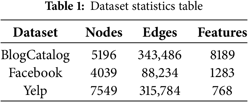
The proposed method was evaluated on three publicly available social network datasets: BlogCatalog [20], Facebook [21], and Yelp.

The BlogCatalog and Facebook datasets consist of user relationship networks obtained from their respective platforms. In both datasets, nodes represent users, and edges denote following relationships. Node features include users’ personalized content, such as blog posts, image tags, and custom labels.

The Yelp dataset is generated from Yelp.com. It contains user relationship and content information extracted from the Yelp platform, including user posts and connections. It is modeled as a user relationship network, where nodes represent users and edges denote friendships. Bert [22] was employed to extract features from user posts, resulting in 768-dimensional vectors used as node features. Prior research noted missing user relationships in the dataset, making it infeasible to use the entire graph for experimentation. Therefore, in line with the experimental setup in, we select the largest connected subgraph with the most nodes as the experimental dataset.

The statistical information of the two datasets is shown in Table 1.

4.2 Dataset Annotation

Among the three datasets, Yelp explicitly designates widely recognized users as “elite,” which aligns with our definition of influential users. Therefore, we select users who have been designated as “elite” by the platform as influential users. However, the BlogCatalog and Facebook datasets do not have annotations for influential users. We employ the SIR (Susceptible–Infected–Recovered) model [23], which is widely used in prior studies [14–16] for simulating influence propagation and annotating influential users.

The SIR Model is a classical epidemiological dynamics model used to simulate the spread of diseases or information within a population. Its core mechanism divides individuals in the network into three states: susceptible (S), infected (I), and recovered (R). In the model, susceptible individuals (users who have not received the information) transition to the infected state (users influenced by the information) at an infection rate I. Infected individuals then transition to the recovered state (the information becomes outdated for the user, and the user no longer pays attention to it) at a recovery rate r. The diffusion scope and speed of disease or information spread are dynamically depicted through stochastic simulations.

Using the SIR Model to label influential users possesses inherent impartiality, primarily manifested in its objective simulation mechanism based on propagation dynamics. Firstly, the SIR Model evaluates all nodes following uniform infection and recovery rates, without presupposing any subjective weights related to node attributes or positions, thereby avoiding artificially introduced structural biases. Secondly, by calculating the average influence of nodes through a large number of stochastic simulations, it can eliminate deviations caused by the randomness of propagation paths, enabling the results to reflect the true propagation potential of nodes. Compared with methods based on static topological features (such as degree centrality), the SIR Model directly simulates the dynamic propagation process, more closely aligning with the causal logic of real-world information diffusion. Therefore, its evaluation results do not rely on a priori assumptions about the network structure. This mechanism, based on uniform rules and probabilities, ensures the fairness and impartiality of the annotation results.

In the specific annotation process, the hyperparameter recovery rate r in the SIR Model is set to 1, and the infection rate I=1.2∗Ith, where Ith is the infection threshold, and Ith=1⟨k2⟩/⟨k⟩−1. Here, ⟨k⟩ and ⟨k2⟩ represent the average degree and the second-order average degree of nodes, respectively. The model is run 1000 times to calculate the average SIR value for each node. The top 10% of nodes ranked by their average SIR values are selected as influential users.

4.3 Experimental Setup

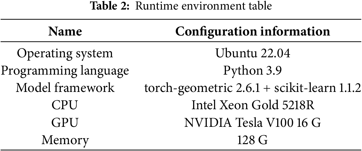
The experimental operating environment is detailed in Table 2. In addition, the hyperparameter α=0.1 for constructing positive and negative sample pairs represents selecting the top 10% of users in terms of centrality ranking as the positive class. The output dimensions of the two-layer GCN in the encoder are 512 and 256, respectively, the output dimension of the fully connected layer is 128, and the temperature coefficient in InfoNCE is β=0.07.

We use the F1 value as the evaluation metric. The F1 values is a commonly used metric in machine learning, particularly for imbalanced classification tasks. It is defined as the harmonic mean of precision and recall, providing a more balanced evaluation of model performance. As shown in Formula (11):

F1=2∗Pression∗RecallPression+Recall(11)

where Pression is the precision rate, representing the proportion of correctly identified influential users among the identified influential users. Recall is the recall rate, representing the proportion of influential users that the method can identify among all influential users.

4.4 Comparative Experiment

To comprehensively demonstrate the effectiveness of this method in identifying influential users and their performance with a small amount of training data, we select 10% to 80% of the data (in increments of 10%) as the training set, and use the remaining data as the test set. Observe the performance of this method and the comparison methods under different proportions of training data. The selected comparison methods are as follows:

EVC [3]: A centrality-based method that does not require training. It assesses node influence based on degree centrality, k-shell values, and shortest path distances. Similarly, we select the top 10% of nodes as influential users. Since this method does not require training, we take its performance on the entire dataset as a baseline.

DeepInf [7]: A GNN-based approach that uses 75% of the data for training in its original implementation. It predicts the social influence of users through random walks and graph attention networks (GAT).

InfGCN [8]: This method is based on convolutional neural networks. In the original paper, 80% of the training set was used for training. It determines the relationship weight based on the betweenness centrality of nodes and uses the splicing of four centrality indicators and user features. It uses GCN to identify influential users.

OlapGN [24]: This method is based on GNNs. In the original paper, 80% of the training set was used for training. It posits that users located in overlapping communities are more likely to be influential users. The method concatenates the detection results of node overlapping communities, centrality metrics, and user features, utilizing GCN to identify influential users.

Table 3 and Fig. 2 summarize the performance of each method under varying proportions of training data. Notably, as the EVC method directly computes node influence without involving model initialization or stochastic processes, its results are consistent across runs, yielding a standard deviation of zero. In contrast, our method, as well as DeepInf, InfGCN, and OlapGN—all of which are GNN-based—were independently run five times under identical hardware conditions. The reported results represent the mean values with corresponding standard deviations.

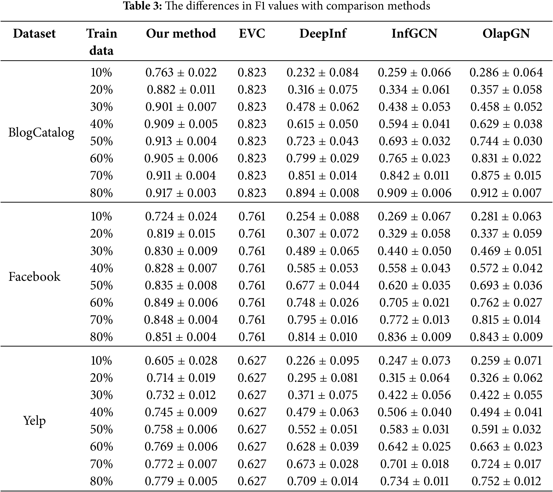
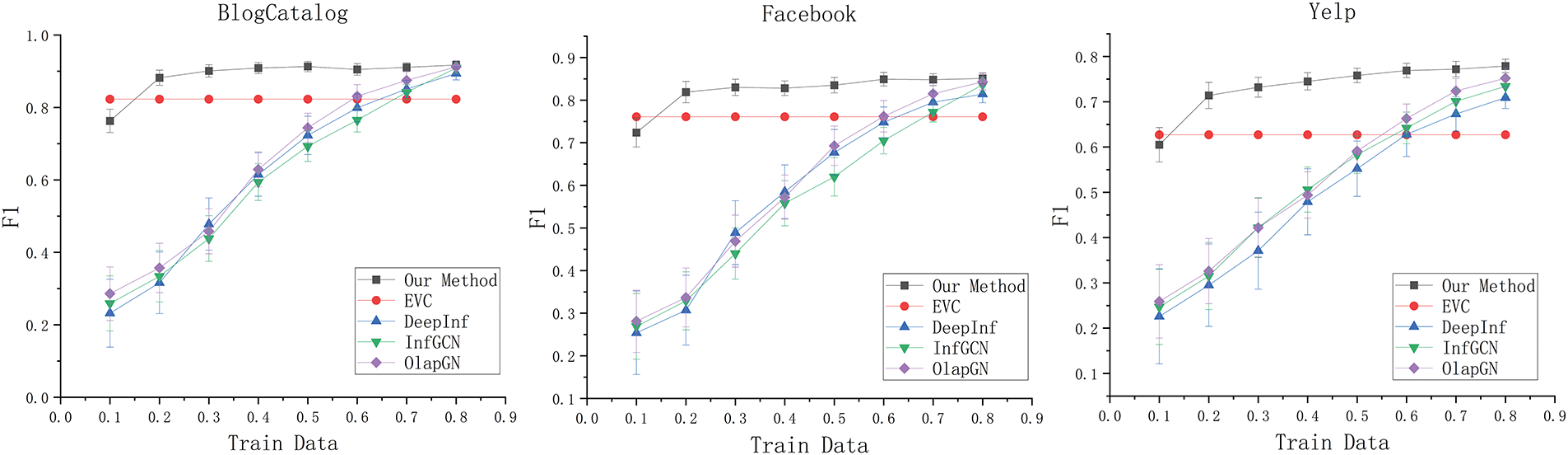
Figure 2: The differences in F1 values with comparison methods

As can be observed from Table 3 and Fig. 2. When only 10% of the training data is used, the F1 values of this method on three different data sets reach 0.763, 0.724, and 0.605, which are comparable to the effects of DeepInf, InfGCN, and OlapGN when using 60% of the training data. When 20% of the training data is used, the F1 values of this method on three different data sets reach 0.882, 0.819, and 0.714. Compared to EVC, the F1 values are improved by 5.9%, 5.8%, and 8.7%, which is comparable to the performance of DeepInf, InfGCN, and OlapGN using 80% of the training data. Furthermore, across all training ratios, our method consistently exhibits lower standard deviation than the other GNN-based approaches. Specifically, when utilizing only 10% of the training data, the standard deviations of the F1 values for our method on the three datasets are merely 0.022, 0.024, and 0.028, respectively. This represents a reduction of 4.2%, 3.9%, and 4.3% compared to the standard deviations of the best-performing alternative methods. Such findings underscore the robust stability of our method even when confronted with limited data.

Comparative experimental results show that:

(1)   The results of graph neural network-based methods such as DeepInf, InfGCN, and OlapGN are better than EVC methods based on network structure. After full training of the method based on graph neural network, its F1 value is eventually greater than that of the EVC method using only structural features, which indicates that the method combining network features and user characteristics using graph neural network can identify influential users more accurately and comprehensively.

(2)   When only a small amount of labeled data is used in this method, it can achieve the effect that other methods use a large amount of labeled data for training. Compared with the graph neural network-based method, which needs to extract features that can distinguish different users from the original user data and map these features into the class space to complete the classification, this method has obtained features that can distinguish different users through comparative learning without annotating data. At this time, only a small amount of data is needed to fine-tune the classifier and map these features into the class space. Therefore, the method in this paper can achieve the effect of DeepInf, InfGCN, and OlapGN using 80% training data at 20% training data.

(3)   The F1 value of all methods increases with the increase of training data, and the growth of F1 value slows down to a certain extent. This is because the influential user identification method needs to capture the common features of influential users from the training data. When the training data is small, the features captured by the method cannot represent the overall trend of influential users, and the F1 value is small. With the increase of training data, the F1 value keeps increasing, and when the training data reaches a certain level, the method can better capture the common characteristics of influential users, and then the increase of training data will lead to a slow increase in F1 value.

4.5 Ablation Experiments

To evaluate the contribution of the three representation vectors extracted by the proposed encoders, we conduct two sets of ablation experiments. The first set involves removing each of the three representation vectors individually and observing the decrease in F1 values resulting from each removal. The second set ablates two of the three vectors, retaining only one, to assess the method’s performance when relying on a single type of representation.

In the first set of ablation experiments, Our Method represents the complete method, while H(s), H(c), and H(g) represent the features reflecting the user’s self-influence, community influence, and global influence extracted by the encoder f1, f2 and f3, respectively. The “-” indicates removing this feature from the complete method. The experiment was conducted five times in total, with the mean value taken as the final result, and the standard deviation was calculated. The experimental results are shown in Fig. 3.

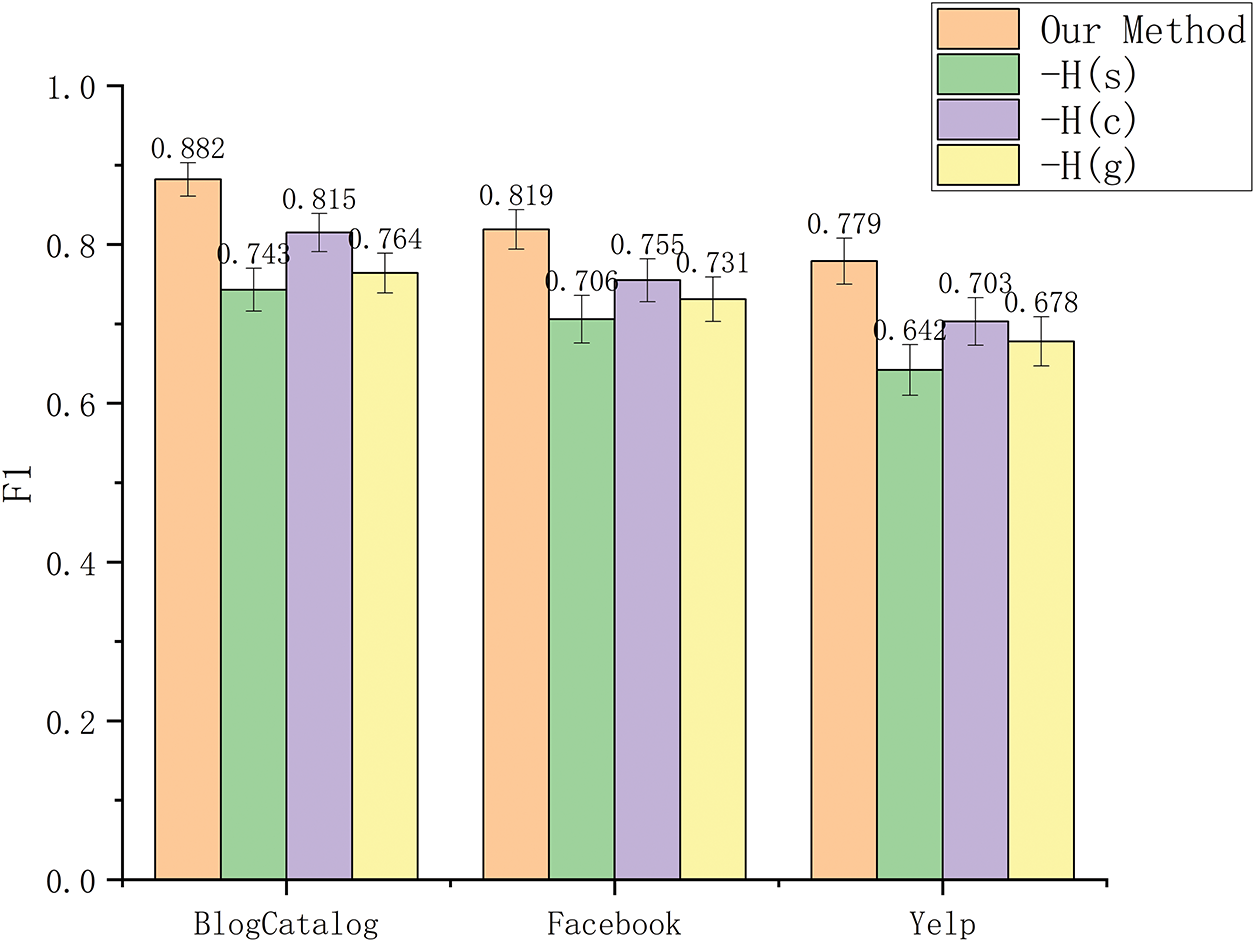
Figure 3: The F1 value after the ablation of different representation vectors

Fig. 3 shows the ablation results of the three representation vectors. In the three datasets, after ablating H(s), the F1 value of the method drops the most, which are 13.9%, 11.3%, and 13.7%, respectively. When H(g) is removed, the F1 values decreases by 11.8%, 8.8%, and 10.1%, indicating its secondary contribution. This proves that most influential users are located inside the network rather than at the network edge. Removing H(c) results in the smallest decline in F1 values—6.7%, 6.4%, and 7.6%—suggesting that community influence contributes the least among the three. After the ablation of each method, F1 values decreased, indicating that each representation vector helped identify influential users.

Ablation results show that:

(1)   After the user’s self-influence feature H(s) extracted by the centrality of use was dissolved, the F1 value of the method decreased the most. The characteristics of influential users are as follows: Users can quickly spread information to different users. H(s) relies on node degree centrality extraction, and a large degree of centrality means that users can quickly disseminate information to different users.

(2)   After the global influence feature H(g) extracted by the k-score was dissolved, the F1 value of the method decreased many times. Users at the center of the network can also quickly spread information to different users in most cases. However, some users in the center of the network may only have connections to fewer nodes, which limits the speed at which they can spread information.

(3)   After the community influence feature H(c) extracted using the value of the number of communities belonging to adjacent nodes is dissolved, the F1 value of the method decreases the least. H(c) relies on the number of communities connected by nodes for extraction, which is a “bridge” node in information dissemination. Its main function is to spread the spread range of information, but it may not be able to spread information quickly.

To further validate the effectiveness of the three extracted representation vectors, we simultaneously ablate two of the three vectors, retaining only one, while also removing the attention network in influential user identification. Instead, only a fully connected layer with an output dimension of 1 and a sigmoid function is used as the classifier. Here, “Our Method” represents the complete method, while “Our Method(H(s))”, “Our Method(H(c))”, and “Our Method(H(g))” respectively represent methods that retain only the features reflecting the user’s self-influence H(s), community influence H(c), and global influence H(g). The experiment was conducted five times in total, with the mean value taken as the final result, and the standard deviation was calculated. The experimental results are shown in Fig. 4.

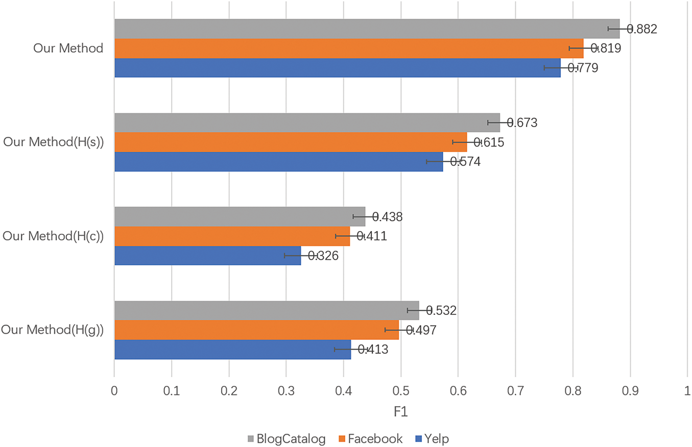
Figure 4: The F1 value after the single representation vector is retained

Fig. 4 presents the F1 value of the method when only one representation vector is retained. Across both datasets, the highest F1 value are achieved when only H(s) is retained, with values of 0.673, 0.615, and 0.574, respectively. Next, the second-highest F1 value is obtained when only H(g) is retained, at 0.532, 0.497, and 0.413, respectively. The lowest F1 value are observed when only H(c) is retained, also at 0.438, 0.411, and 0.326. Considering that influential users constitute only 10% of the three datasets, the F1 value for random guessing in this scenario is 16.7%. The fact that the F1 values of methods using only one representation vector are all higher than this indicates that all three learned representation vectors help identify influential users.

The experimental results show that:

(1)   The highest F1 value is achieved when only the user’s self-influence feature H(s), extracted using degree centrality, is retained. This suggests that the differences between influential users and ordinary users are more pronounced in terms of the user’s self-influence, i.e., the number of users related to the user, including the user’s followers, friends who make comments, etc. Such users possess strong information dissemination capabilities.

(2)   The second-highest F1 value is obtained when only the user’s global influence feature H(g), extracted using the k-score value, is retained. This may be because the topological position of nodes located at the center of the network determines that the information they disseminate can reach most areas of the network in many cases. However, compared to nodes with a high degree of centrality, their dissemination speed may be slower.

(3)   The lowest F1 value is observed when only the user’s community influence feature H(c), extracted using the number of communities that adjacent nodes belong to, is retained. This may be because in some cases, influential users are also well-informed users who gain higher influence by forwarding information across different communities and facilitating information dissemination. However, this subset of influential users constitutes a smaller proportion.

4.6 Hyperparameter Sensitivity Experiments

To evaluate the sensitivity of the proposed method to different hyperparameter settings, we analyze two key hyperparameters: (1) the hyperparameter α, which controls the proportion of positive samples selected, and (2) the temperature coefficient β in the contrastive learning loss function. Each experiment was independently repeated five times under identical hardware conditions, and the results are presented as the mean values along with their standard deviations.

(1) Positive Sample Ratio α

The hyperparameter α controls the proportion of positive samples selected when using centrality metrics to distinguish between positive and negative samples. Accurate selection of positive and negative samples significantly impacts the model’s performance. In this section, we set α to the following values: 0.05, 0.1, 0.2, 0.3, 0.4, 0.5, 0.6, 0.7, 0.8, and 0.9. The experimental results are depicted in Fig. 5a.

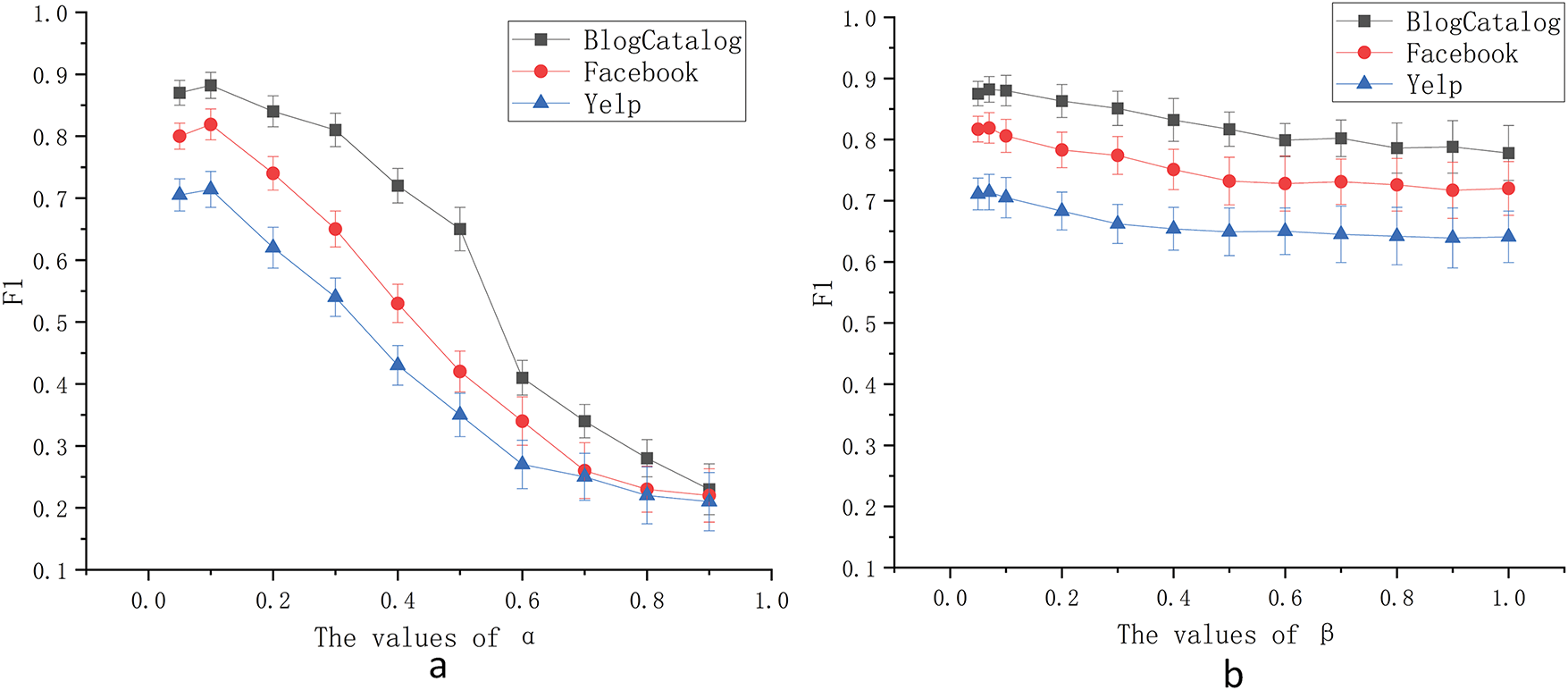
Figure 5: The influence of different parameters on the F1 value. (a) The values of α. (b) The values of β

Experimental results show that as α increases, the F1 values initially improves. However, once α exceeds 0.1, the F1 value begins to decline gradually. Consequently, the positive sample ratio of the method is set to 0.1. In the BlogCatalog and Facebook datasets, influential users account for approximately 10% of all users, while in the Yelp dataset, this proportion is 11.6%, which is also close to 0.1. When α exceeds the true proportion of influential users in the dataset, ordinary users may be mistakenly selected as positive samples based on centrality metrics, which can mislead the model during training and degrade identification accuracy. Conversely, if α is set higher than the actual proportion of influential users, some influential users might be incorrectly classified as negative samples, preventing the model from learning the characteristics of certain influential users. Therefore, α should be set close to the empirical proportion of influential users in the dataset for optimal performance.

(2) Temperature Coefficient β

The hyperparameter β controls the degree of focus on hard negative samples in the contrastive loss function [19]. Lower values of β amplify the gradients for hard negative samples, causing the method to pay more attention to these less frequent hard negative samples. In this section, we set β to the following values: 0.05, 0.07, 0.1, 0.2, 0.3, 0.4, 0.5, 0.6, 0.7, 0.8, 0.9, and 1.0. The experimental results are illustrated in Fig. 5b.

Experimental results indicate that as β increases, the F1 values initially improves. However, once β exceeds 0.07, the F1 value gradually declines. The method achieves its best performance when β is set to 0.07. Therefore, the temperature coefficient of the method is configured to be 0.07. In the three datasets, BlogCatalog and Facebook, influential users are identified using the SIR model, which is widely recognized as an effective approach for labeling influential users and is also applicable to the Yelp dataset. This leads to similar scenarios of hard negative samples across the three datasets, hence the same value of β is used. Nevertheless, since this value lacks a concrete physical meaning, it needs to be readjusted in practical applications.

5  Discussion

In this section, we focus on three main areas of discussion:

(1)   We examine the rationale behind selecting the three metrics in our proposed approach, along with potential biases they might introduce and strategies to address them.

(2)   We conduct a further comparison between our method and baseline approaches in terms of runtime and memory usage and discuss their applicability in large-scale networks.

(3)   We delve into the potential biases that could result from using the SIR model for data labeling.

5.1 Analysis of Influence Metrics

The ablation experiments demonstrate the effectiveness of the three influence metrics employed in our method. However, there is a lack of further justification for the rationality of choosing these three metrics. Next, we will demonstrate the rationality of our method from three aspects, namely: the necessity of selecting three types of influence with different scopes of action, the corresponding indicators for each type of influence, as well as the deviations of each indicator under certain circumstances and possible solutions.

We categorize user influence into three levels based on its scope of action: self-influence, community influence, and global influence. This classification method is widely applied in the field of influential user identification. Self-influence manifests in small-scale interpersonal interactions. Although its scope is limited, it possesses a high degree of precision and emotional penetration, often leading to immediate feedback or behavioral changes. Community influence operates within specific groups or platforms, demonstrating users’ discourse power and leadership in forums, industry communities, or interest groups. Global influence, on the other hand, extends to a broader social level. Users with such influence can trigger cross-community discussions through media dissemination, public event statements, etc., with their impact being enduring and diffusive.

To effectively capture these levels of influence, we adopt degree centrality, the number of communities connected by neighboring nodes, and the k-core value as representative indicators. Among these, degree centrality best reflects self-influence as it directly measures the number of direct connections an individual has in a social network. Within a local scope, influence often hinges on a user’s ability to interact directly with surrounding nodes, and degree centrality, focusing on the scale of direct associations, aligns with the characteristics of local influence. The number of communities connected by adjacent nodes best reflects community influence, as it directly mirrors the user’s bridging role across different groups. In a social network, if a user’s adjacent nodes are distributed across different communities, the community distribution of adjacent nodes directly quantifies the user’s potential to break down information silos and integrate diverse groups. The k−core value best reflects global influence, as it measures the depth of a user’s representation vector within the network’s core layer, rather than simply the breadth of connections. Nodes with high k−core values are often situated in highly interconnected core circles. These nodes not only possess a large number of connections themselves but also have neighbors that are similarly located in highly connected subgraphs, forming stable influence hubs. By iteratively peeling away peripheral nodes, the k−core value screens out users truly positioned at the network’s core hubs, thus more accurately reflecting their enduring influence and information dissemination potential on a global scale. Although this paper selects the most representative indicators to represent different types of user influence, there may still be deficiencies when facing different types of networks.

We use degree centrality to evaluate the self-influence of users. Nevertheless, in networks with edge weights, the importance of edges varies, and the number of edges cannot fully represent a node’s influence. A node with a smaller total number of edges but including important edges may actually be more influential than a node with a larger total number of edges. In such cases, metrics like Eigenvector Centrality, which consider the importance of both nodes and edges, might be a better choice. However, it is worth noting that determining edge weights requires more user information, which may be difficult to obtain in practical scenarios. Therefore, in most cases, selecting degree centrality is a reasonable approach.

We use the number of communities connected by adjacent nodes to evaluate a node’s community influence. However, this metric relies on the accuracy of community detection algorithms. When evaluating influential nodes in dynamically evolving networks such as transportation networks, due to the rapid changes in community structures, this metric may misestimate a node’s ability to span across communities. In such cases, metrics like Structural Hole Constraint, which do not depend on community partitioning, might be a better choice. However, for social networks, where user behaviors span long periods and community structures adjust slowly, using this metric to judge a node’s community influence is reasonable.

We use the k−core value is selected to evaluate a node’s global influence, emphasizing the depth of a node’s representation within the core-periphery structure. However, in networks with less prominent hierarchical characteristics, such as uniform random networks, this metric may not effectively distinguish between different levels of node influence. In such cases, metrics like Neighborhood Coreness [25], which consider more node information, might be a better choice. Nevertheless, social networks differ significantly from uniform random networks, as their node degree distributions follow a power-law distribution. This leads to a substantial gap between the k-core values of highly influential nodes and ordinary nodes, making the computational complexity of using k−core lower in such scenarios.

5.2 Analysis of Computational Complexity

This section compares the computational complexity of our method with four baseline approaches, namely EVC, DeepInf, InfGCN, and OlapGN, which were utilized in the experimental section. Additionally, we discuss the applicability of these methods in large-scale networks.

For the proposed method in this paper, the computational cost mainly arises from three components: the calculation of centrality-related measures during the construction of positive and negative sample pairs, the aggregation operations of the graph neural network in the user encoding phase, and the training of the final classifier. In the phase of constructing positive and negative sample pairs, three centrality metrics are employed, resulting in a computational complexity of O(n)+O(nlog⁡(n))+O(n)≈O(nlog⁡(n)), where n denotes the number of nodes. In the user encoding phase, each layer requires a matrix multiplication operation between the adjacency matrix and the node feature matrix to aggregate the neighbor features of each node, yielding a computational complexity of O(n∗E∗F), where E represents the number of edges and F denotes the feature dimension. During the training of the classifier, the computational complexity is O(m∗s∗d2), where m<n is the number of nodes participating in the classifier training, sis the number of features per node, and d is the length of each node’s representation. In summary, the total computational complexity of the proposed method is O(nlog⁡(n)+n∗E∗F+s∗d2).

For the four comparative methods, the EVC method has a computational complexity of O(n2). The DeepInf method exhibits a computational complexity of O(n∗K∗F), where K<E represents the size of the sampled neighborhood, a hyperparameter in the DeepInf method. For the InfGCN method, which utilizes centrality metrics in constructing user representation vector, the time cost arises from both user feature construction and the graph neural network. Due to the use of betweenness centrality, the computational complexity for user feature construction is O(n3), leading to an overall computational complexity of O(n3+n∗E∗F) for InfGCN. For the OlapGN method, the time consumption originates from three parts: community identification, user feature construction, and the graph neural network. Similar to InfGCN, it employs betweenness centrality, resulting in a computational complexity of O(n3) for user feature construction. Additionally, OlapGN involves community partitioning of nodes, leading to an overall computational complexity of O(n3+nlog⁡(n)+n∗E∗F).

In terms of computational complexity, the proposed method exhibits a higher computational complexity compared to the EVC and DeepInf methods. This is primarily attributed to the necessity of calculating node centrality to construct positive and negative sample pairs and the utilization of an attention network to fuse multiple user features, which collectively increase the method’s computational complexity. However, the proposed method’s computational complexity is lower than that of the InfGCN and OlapGN methods, indicating that it achieves superior performance while maintaining a moderate computational complexity, thereby demonstrating its advantages.

To further illustrate the practical feasibility of the proposed method, Table 4 presents the runtime duration and memory consumption. Specifically, the runtime duration is the aggregate time consumed across all phases of the method, while the memory consumption denotes the maximum memory utilization during the execution process.

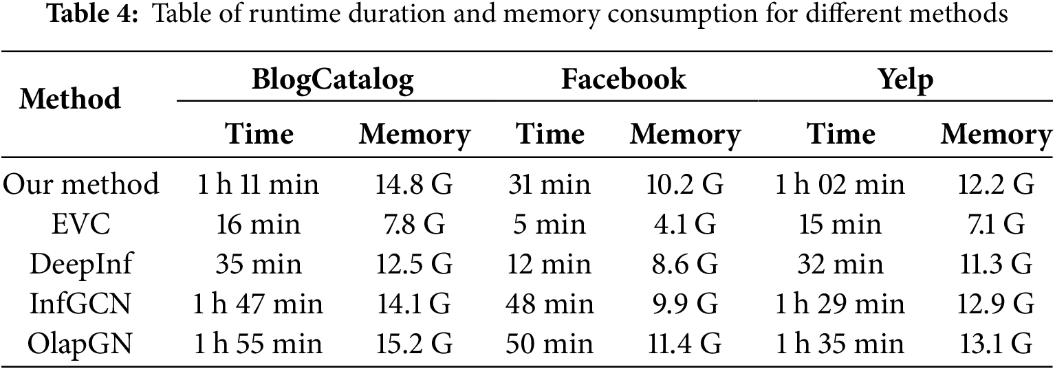
In Table 4, it is evident that the EVC and DeepInf methods exhibit superior performance in terms of runtime duration and memory consumption, whereas our proposed method, along with methods like InfGCN and OlapGN, demonstrates relatively poorer performance in these aspects. This discrepancy can be attributed to the substantial computational demands of GNNs when dealing with large-scale networks. The EVC method, being based on centrality metrics, does not rely on GNNs, thereby circumventing the associated computational overhead. In contrast, the DeepInf method incorporates optimizations in its utilization of GNNs by manually specifying the size of the sampled neighborhood, which effectively reduces the runtime duration and memory consumption of the GNN. Consequently, the EVC and DeepInf methods demonstrate better adaptability to large-scale networks, whereas our proposed method is not ideally suited for applications involving large-scale networks.

5.3 Potential Biases Introduced by the SIR Model

We employ the SIR model to label influential users in the BlogCatalog and Facebook datasets, which may introduce potential biases. Although the effectiveness of the proposed method has been validated using the Yelp dataset, it is still necessary to be cautious about the deviations that may arise from the SIR model, particularly its notable limitations in dynamic network environments.

Firstly, the SIR model assumes that the transmission and recovery probabilities are fixed and homogeneous. However, in reality, user influence often dynamically changes with content, context, and relationship strength, leading to static parameters that may overestimate the propagation capacity of core nodes or underestimate the potential explosiveness of peripheral nodes. Secondly, the SIR model implicitly assumes a static network structure, whereas in actual social networks, user connections evolve in real-time in response to events—the sudden formation of new edges or the invalidation of old edges may cause the model to underestimate emerging key users. More critically, the SIR model relies on a single “infection” propagation mode, neglecting the heterogeneity of user behaviors and the interference of competing information flows. It is important to emphasize that the method proposed in this paper is designed solely for static networks and cannot be applied to dynamic networks.

6  Conclusion

This paper proposes a method for influential user identification based on semi-supervised contrastive learning. The method employs a GCN as an encoder to integrate user features and structural information. Positive and negative samples are constructed based on centrality metrics to guide the encoder in generating multiple influence-aware representation vectors. An attention network is then used to fuse these representation vectors, enabling accurate identification of influential users even with a small amount of labeled data. Experiments on real-world social network datasets show that our method achieves comparable F1 values to GNN-based baselines trained with 80% labeled data, while using only 20%, thus demonstrating its effectiveness.

However, the method has two main limitations: it relies on centrality-based sample construction, making its performance sensitive to the choice of metrics, and it requires access to user relationships and attributes, which may be difficult to obtain in real-world settings. Future work will explore identifying influential users using only user-generated content, particularly in scenarios where relational and attribute information is unavailable.

Acknowledgement: The authors would like to thank the editors for their valuable comments and kind support during the review process.

Funding Statement: This work was supported by the National Key Project of the National Natural Science Foundation of China under Grant No. U23A20305.

Author Contributions: The authors confirm contribution to the paper as follows: Jialong Zhang: Conceptualization, Methodology, Investigation, Writing. Meijuan Yin: Writing, Reviewing & Editing. Yang Pei, Fenlin Liu and Chenyu Wang: Review & Editing. All authors reviewed the results and approved the final version of the manuscript.

Availability of Data and Materials: All the data used in this study are obtained from publicly available benchmark datasets, which are appropriately cited in the manuscript.

Ethics Approval: Not applicable.

Conflicts of Interest: The authors declare no conflicts of interest to report regarding the present study.

References

1. Wu S, Li W, Shen H, Bai Q. Identifying influential users in unknown social networks for adaptive incentive allocation under budget restriction. Inf Sci. 2023;624:128–46. doi:10.1016/j.ins.2022.12.071. [Google Scholar] [CrossRef]

2. Zhao J, He H, Zhao X, Lin J. Modeling and simulation of microblog-based public health emergency-associated public opinion communication. Inf Process Manag. 2022;59(2):102846. doi:10.1016/j.ipm.2021.102846. [Google Scholar] [PubMed] [CrossRef]

3. Rashid Y, Bhat JI. Topological to deep learning era for identifying influencers in online social networks: a systematic review. Multimed Tools Appl. 2024;83(5):14671–714. doi:10.1007/s11042-023-16002-8. [Google Scholar] [CrossRef]

4. Ullah A, Wang B, Sheng J, Khan N. Escape velocity centrality: escape influence-based key nodes identification in complex networks. Appl Intell. 2022;52(14):16586–604. doi:10.1007/s10489-022-03262-4. [Google Scholar] [CrossRef]

5. Ou Y, Guo Q, Xing JL, Liu JG. Identification of spreading influence nodes via multi-level structural attributes based on the graph convolutional network. Expert Syst Appl. 2022;203:117515. doi:10.1016/j.eswa.2022.117515. [Google Scholar] [CrossRef]

6. Alghobiri M. Exploring the attributes of influential users in social networks using association rule mining. Soc Netw Anal Min. 2023;13(1):118. doi:10.1007/s13278-023-01118-4. [Google Scholar] [CrossRef]

7. Khare P, Shekhar R, Karan M, McQuistin S, Perkins C, Castro I, et al. Tracing linguistic markers of influence in a large online organisation. In: Proceedings of the 61st Annual Meeting of the Association for Computational Linguistics (Volume 2: Short Papers); 2023 Jul 9–14; Toronto, ON, Canada. p. 82–90. doi:10.18653/v1/2023.acl-short.8. [Google Scholar] [CrossRef]

8. Li W, Xu Z, Sun Y, Gong Q, Chen Y, Ding AY, et al. DeepPick: a deep learning approach to unveil outstanding users with public attainable features. IEEE Trans Knowl Data Eng. 2021;35(1):291–306. doi:10.1109/TKDE.2021.3091503. [Google Scholar] [CrossRef]

9. Daneshfar F, Saifee BS, Soleymanbaigi S, Aeini M. Elastic deep multi-view autoencoder with diversity embedding. Inf Sci. 2025;689:121482. doi:10.1016/j.ins.2024.121482. [Google Scholar] [CrossRef]

10. Qiu J, Tang J, Ma H, Dong Y, Wang K, Tang J. DeepInf: social influence prediction with deep learning. In: Proceedings of the 24th ACM SIGKDD International Conference on Knowledge Discovery & Data Mining; 2018 Aug 19–23; London, UK. p. 2110–9. doi:10.1145/3219819.3220077. [Google Scholar] [CrossRef]

11. Zhao G, Jia P, Zhou A, Zhang B. InfGCN: identifying influential nodes in complex networks with graph convolutional networks. Neurocomputing. 2020;414(11):18–26. doi:10.1016/j.neucom.2020.07.028. [Google Scholar] [CrossRef]

12. Jain L, Katarya R, Sachdeva S. Opinion leaders for information diffusion using graph neural network in online social networks. ACM Trans Web. 2023;17(2):1–37. doi:10.1145/3580516. [Google Scholar] [CrossRef]

13. Kipf TN, Welling M. Semi-supervised classification with graph convolutional networks. In: Proceedings of the 5th International Conference on Learning Representations (ICLR); 2017 Apr 24–26; Toulon, France. [Google Scholar]

14. Curado M, Tortosa L, Vicent JF. A novel measure to identify influential nodes: return random walk gravity centrality. Inf Sci. 2023;628(5):177–95. doi:10.1016/j.ins.2023.01.097. [Google Scholar] [CrossRef]

15. Zhang Q, Shuai B, Lü M. A novel method to identify influential nodes in complex networks based on gravity centrality. Inf Sci. 2022;618(5996):98–117. doi:10.1016/j.ins.2022.10.070. [Google Scholar] [CrossRef]

16. Namtirtha A, Dutta B, Dutta A. Semi-global triangular centrality measure for identifying the influential spreaders from undirected complex networks. Expert Syst Appl. 2022;206(1):117791. doi:10.1016/j.eswa.2022.117791. [Google Scholar] [CrossRef]

17. Daneshfar F, Soleymanbaigi S, Yamini P, Amini MS. A survey on semi-supervised graph clustering. Eng Appl Artif Intell. 2024;133(2):108215. doi:10.1016/j.engappai.2024.108215. [Google Scholar] [CrossRef]

18. Blondel VD, Guillaume JL, Lambiotte R, Lefebvre E. Fast unfolding of communities in large networks. J Stat Mech. 2008;2008(10):P10008. doi:10.1088/1742-5468/2008/10/p10008. [Google Scholar] [CrossRef]

19. He K, Fan H, Wu Y, Xie S, Girshick R. Momentum contrast for unsupervised visual representation learning. In: 2020 IEEE/CVF Conference on Computer Vision and Pattern Recognition (CVPR); 2020 Jun 13–19; Seattle, WA, USA. p. 9726–35. doi:10.1109/cvpr42600.2020.00975. [Google Scholar] [CrossRef]

20. Rossi R, Ahmed N. The network data repository with interactive graph analytics and visualization. In: Proceedings of the 29th AAAI Conference on Artificial Intelligence; 2015 Jan 25–30; Austin, TX, USA. p. 4292–3. doi:10.1609/aaai.v29i1.9277. [Google Scholar] [CrossRef]

21. McAuley J, Leskovec J. Learning to discover social circles in ego networks. In: Pereira F, Burges CJC, Bottou L, Weinberger KQ, editors. Advances in Neural Information Processing Systems 25 (NIPS 2012); 2012 Dec 3–6; Lake Tahoe, NV, USA. p. 539–47. [Google Scholar]

22. Devlin J, Chang MW, Lee K, Toutanova K. Bert: pre-training of deep bidirectional transformers for language understanding. In: Proceedings of the 2019 Conference of the North American Chapter of the Association for Computational Linguistics: Human Language Technologies, NAACL-HLT 2019; 2019 Jun 2–7; Minneapolis, MN, USA. p. 4171–86. doi:10.18653/v1/N19-1423. [Google Scholar] [CrossRef]

23. Kephart JO, White SR. Measuring and modeling computer virus prevalence. In: Proceedings 1993 IEEE Computer Society Symposium on Research in Security and Privacy; 1993 May 24–26; Oakland, CA, USA. doi:10.1109/RISP.1993.287647. [Google Scholar] [CrossRef]

24. Rashid Y, Bhat JI. OlapGN: a multi-layered graph convolution network-based model for locating influential nodes in graph networks. Knowl Based Syst. 2024;283(1):111163. doi:10.1016/j.knosys.2023.111163. [Google Scholar] [CrossRef]

25. Kumar S, Panda BS. Identifying influential nodes in social networks: neighborhood coreness based voting approach. Phys A Stat Mech Appl. 2020;553(3):124215. doi:10.1016/j.physa.2020.124215. [Google Scholar] [CrossRef]