Anomaly Diagnosis Using Machine Learning Method in Fiber Fault Diagnosis

1  Introduction

Optical Time Domain Reflectometer (OTDR) technology has been a cornerstone in the field of optical fiber monitoring and fault analysis for decades. Traditional methods, such as the two-point method combined with least squares fitting, have been widely used for estimating event location and loss in OTDR traces by calculating the best-fit line between two markers [1]. While simple, these methods suffer from limited accuracy in noisy environments, making them less suitable for modern optical networks with increasingly stringent reliability requirements.

To address these limitations, researchers have proposed various advanced techniques. Liu et al. introduced the Gabor Series Representation combined with the Minimum Description Length criterion (GSR/MDL) method and later improved it with the R1MSDE method [2], achieving higher accuracy in event detection by leveraging matched subspace detection theory [3]. Man et al. developed an event detection method based on the Short-Time Fourier Transform (STFT) with an exponential window and binary signal detection theory, which enhanced OTDR’s ability to detect distant events while improving computational efficiency [4]. Furthermore, wavelet transform (WT)-based methods have shown promise due to their scalable spatial resolution [5,6]. However, the computational complexity of WT often hinders their practicality for real-time applications in optical fiber monitoring systems. Subsequently, Kong et al. proposed a hybrid approach combining correlation matching with short-time Fourier transform (STFT) [7], but these methods remain numerically intensive and struggle with low signal-to-noise ratio (SNR) environments.

In recent years, machine learning (ML) techniques have demonstrated strong capabilities in OTDR event analysis. Abdelli et al. [8–10] demonstrated a wide range of applications of Machine Learning techniques for laser failure mode detection, lifetime prediction and reliability enhancement. Abdelli et al. [11] demonstrated the potential of convolutional neural networks (CNNs) for the detection and characterization of reflection events in noisy environments. And, Abdelli et al. also used long and short-term memory networks to detect, localize and estimate the reflectivity of fiber-optic reflection faults (events) including connectors and mechanical splices [12]. In addition, Zhang et al. [13] showed the robustness of deep convolutional neural networks combined with novel training methods in noisy environments, which provides theoretical support for us to deal with noise in OTDR signals. Bidirectional Long Short-Term Memory (BiLSTM) networks have been used to solve the time-dependent problem in OTDR traces for fault detection and localization [14,15], and the combination of CNN and BiLSTM has been shown to perform well in improving the accuracy and robustness of fault diagnosis tasks [14]. The ML models presented in the two publications of [14,15] were trained using experimental data containing faults modeled using optical components such as connectors or reflectors.

As a result, the generalization ability and robustness of these models may be severely degraded when tested with new unseen data, including actual induced faults with a variety of modes, such as fiber bending events generated for different values of bend radius. Furthermore, while these methods distinguish non-reflective events from other events, they cannot readily distinguish failures due to poor splicing or fiber taps. However, most current methods focus on single-scale analysis or rely on fixed feature extraction techniques, making it difficult to adequately capture the multiscale nature of OTDR signals.

In the field of time series anomaly detection, Lu et al. [16] proposed a multiscale Convolutional Long Short-Term Memory (C-LSTM) model that has demonstrated effective performance in detecting anomalies in time series. Motivated by this success, we aim to extend the application of time series analysis techniques to the domain of optical fiber fault detection. In this regard, we optimized the model proposed by Lu et al. [16]. First, the original binary classification framework was modified into a multi-classification framework. Second, the LSTM in the model was replaced with BiLSTM to enhance feature extraction capabilities. This extension seeks to address the challenge of distinguishing faults caused by poor splicing or fiber connectors, which are difficult to identify from OTDR signals using conventional methods. Through experimentation, we propose three multiscale CNN-BiLSTM models: Independent Multiscale CNN-BiLSTM (IMC-BiLSTM), Combined Multiscale CNN-BiLSTM (CMC-BiLSTM), and Shared Multiscale CNN-BiLSTM (SMC-BiLSTM). We observe that replacing the LSTM model with a BiLSTM model significantly improves the performance of our models, with F1 scores increasing by 0.41%, 0.8%, and 0.49% for the respective models. Additionally, we optimize the activation functions of the models and find that the performance is highest when using the ReLU activation function. Finally, we compare our models with existing machine learning algorithms for optical fiber fault detection on the public dataset OTDR_data [17]. Experimental results indicate that the overall performance of our models surpasses that of existing machine learning methods, demonstrating the effectiveness of our approach in enhancing the detection of optical fiber faults.

The main contributions of this paper are summarized as follows:

Proposed Three Multiscale CNN-BiLSTM Deep Learning Models: Three deep learning models of multiscale CNN-BiLSTM (IMC-BiLSTM, CMC-BiLSTM, and SMC-BiLSTM) are proposed, which adopt the structures of independent multiscale CNNs, combined multiscale CNNs, and shared multiscale CNNs, respectively, effectively extracting the multiscale features of OTDR signals. This approach addresses key challenges in optical fiber fault detection, including insufficient accuracy in noisy environments, high misjudgment rates under complex conditions, slow detection speeds, and high equipment costs.

Robustness: The proposed models show high accuracy in classifying different types of optical fiber faults, especially performing excellently in classifying highly significant fault types.

Parameter Optimization: By comparing the model performances under different activation functions, it is found that using ReLU as the hidden layer activation function can achieve the highest F1 score.

The rest of this article is organized as follows: Section 2 introduces the relevant theoretical foundations and other existing deep learning methods. Section 3 describes the three proposed models. Section 4 provides an overview of the experimental setup, including hardware and software configuration, dataset composition, fault categories, training programs, and evaluation metrics. Section 5 introduces the experimental results and compares the three proposed models (IMC-BiLSTM, CMC-BiLSTM, SMC-BiLSTM) with the baseline model. The classification performance is analyzed through confusion matrix, t-SNE visualization, and ROC curve. Finally, Section 6 provides a summary of this study.

2  Related Work

Recent years have witnessed a rapid evolution in OTDR-based fault diagnosis, transitioning from traditional signal processing methods to advanced machine learning and deep learning approaches.

Traditional methods, such as the two-point linear fitting technique and wavelet transform (WT)-based localization, offer basic estimation capabilities but often struggle under noisy or low-SNR conditions [1]. While hybrid signal processing techniques, such as STFT-based correlation matching [7] and Gabor transforms [4], improved performance in specific scenarios, their computational complexity and limited generalization constrained practical applications.

To overcome these limitations, researchers have increasingly turned to machine learning (ML) and deep learning (DL). Abdelli et al. [8–12] applied CNNs and LSTMs to OTDR data, demonstrating improvements in reflection event detection and time-dependent fault localization. Soothar et al. [18] employed advanced machine learning (ML) and deep learning (DL) techniques to detect and classify six different types of optical fiber faults, including fiber cuts, eavesdropping, splices, faulty connectors, bends, and physical contact (PC) connectors. Among the tested models, the hybrid CNN-LSTM architecture achieved the highest accuracy of 99%, demonstrating superior performance. Prakash and Kasthuri [19] proposed a denoising convolutional autoencoder for fault detection in optical fibers, followed by a bidirectional gated recurrent unit (BiGRU) for fault classification and localization. Xu et al. [20] proposed a hybrid model combining CNN-BiLSTM and Convolutional Block Attention Module (CBAM) for identifying and classifying anchor damage events in submarine cables. Zheng et al. [21] proposed a feature extraction algorithm combining Variational Mode Decomposition (VMD), Mel Frequency Cepstral Coefficients (MFCC), and a Backpropagation Neural Network (BPNN) classifier. However, the method utilized a relatively small training dataset, and its feature extraction process requires further optimization. Wu et al. [22] introduced an efficient 1-D CNN architecture with an optimally selected Support Vector Machine (SVM) classifier, offering a novel data-driven recognition approach. Nevertheless, its recognition capability was primarily limited to single vibration events, posing challenges for mixed event detection.

Despite their effectiveness, most existing models suffer from limitations such as: Fixed-size convolution kernels, which restrict the ability to capture multiscale temporal patterns; Shallow architectures with insufficient contextual modeling; Limited performance on complex or mixed fault scenarios; A focus on binary classification or limited fault categories.

In response, we propose three Multiscale CNN-BiLSTM architectures (IMC-BiLSTM, CMC-BiLSTM, and SMC-BiLSTM) to more effectively extract hierarchical spatial-temporal features from OTDR traces. Our models combine multiscale convolutional encoding with bidirectional sequence modeling to better distinguish various fiber fault types. As demonstrated in Section 5, our models outperform the part of methods in F1-score, generalization, and robustness under real-world conditions, validating the necessity of multiscale and deeper architectures in OTDR-based fault diagnosis.

2.1 C-LSTM Model

As shown in Fig. 1. The C-LSTM model [23] features a hierarchical architecture that sequentially integrates convolutional neural networks (CNNs) [24] and long short-term memory (LSTM) [25] networks. The architecture begins with one or more 1D convolutional layers that extract local spatial features through kernel-based filtering operations, followed by pooling layers for dimensionality reduction. These processed features are then fed into stacked LSTM layers that capture temporal dependencies through recurrent connections and gating mechanisms. A distinctive characteristic of C-LSTM is its dual-phase feature learning: the CNN component acts as a spatial feature extractor that identifies local patterns in sliding windows, while the LSTM component models longer-range sequential relationships between these extracted features. The architecture typically concludes with fully connected layers for task-specific output generation.

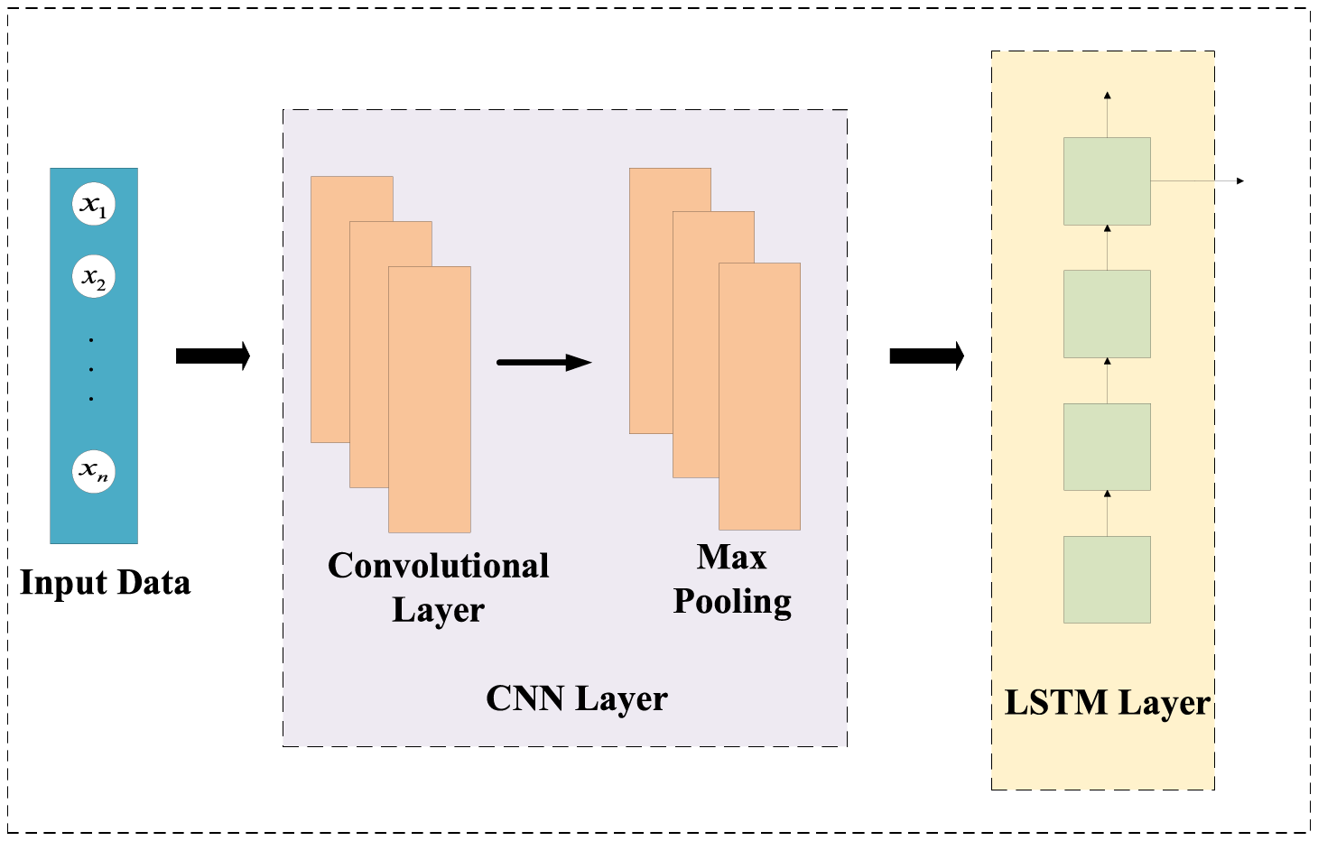
Figure 1: The architecture of C-LSTM

As shown in Fig. 2, each LSTM unit comprises a forget gate (ft), an input gate (it), an output gate (ot), a cell state (ct), and a hidden state (ht). In this equation, wf denotes the weight matrix of the forget gate, xt represents the current input, and bf is the corresponding bias vector. This notation is consistent across the other gates as well. The forget gate determines which parts of the previous cell state should be discarded, allowing the model to forget irrelevant information while retaining critical memory.

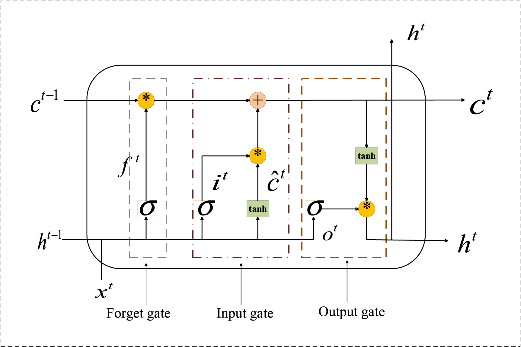
Figure 2: The architecture of LSTM

ft=σ(wf[ht−1,xt]+bf)(1)

The input gate decides which elements of the input should be integrated into the current cell state, ensuring that essential features are retained.

it=σ(wi[ht−1,xt]+bi)(2)

The output gate regulates which information from the current cell state should be included in the hidden state for subsequent processing.

ot=σ(wo[ht−1,xt]+bo)(3)

The combination of these gates and states allows LSTM to dynamically manage and propagate information over time, effectively extracting meaningful temporal features from complex data.

c^t=tan⁡h(wc[ht−1,xt]+bc)(4)

ct=ft∗ct−1+itc^t(5)

ht=ot∗tan⁡h(ct)(6)

2.2 BiLSTM

BiLSTM [26] is an extension of LSTM that helps to improve the performance of the model. It consists of two LSTMs: one forward LSTM model that takes the input in a forward direction, and one backward LSTM model that learns the reversed input. The output yt of the model is generated by combining the forward output ht→ and backward output ht← as described by the following equations.

ht→=LSTM(xtht−1→)(7)

ht←=LSTM(xt,ht−1←)(8)

yt=wht→yht→+wht←yht←+by(9)

2.3 BiGRU

The Gated Recurrent Unit (GRU) [27] is a variant of the traditional Recurrent Neural Network (RNN) architecture, specifically designed to mitigate issues such as vanishing gradients during training [28]. It achieves this by integrating two specialized gating mechanisms—namely, the update gate and the reset gate—which regulate the flow of information through the network. The update gate is responsible for deciding how much of the past information should be carried forward, effectively balancing between retaining historical context and integrating new input. In contrast, the reset gate determines the extent to which previous hidden states are ignored, allowing the model to selectively forget irrelevant information. As illustrated in Fig. 3, this streamlined architecture enables GRUs to efficiently learn temporal dependencies, especially in long sequences, while requiring fewer parameters than traditional LSTM units.

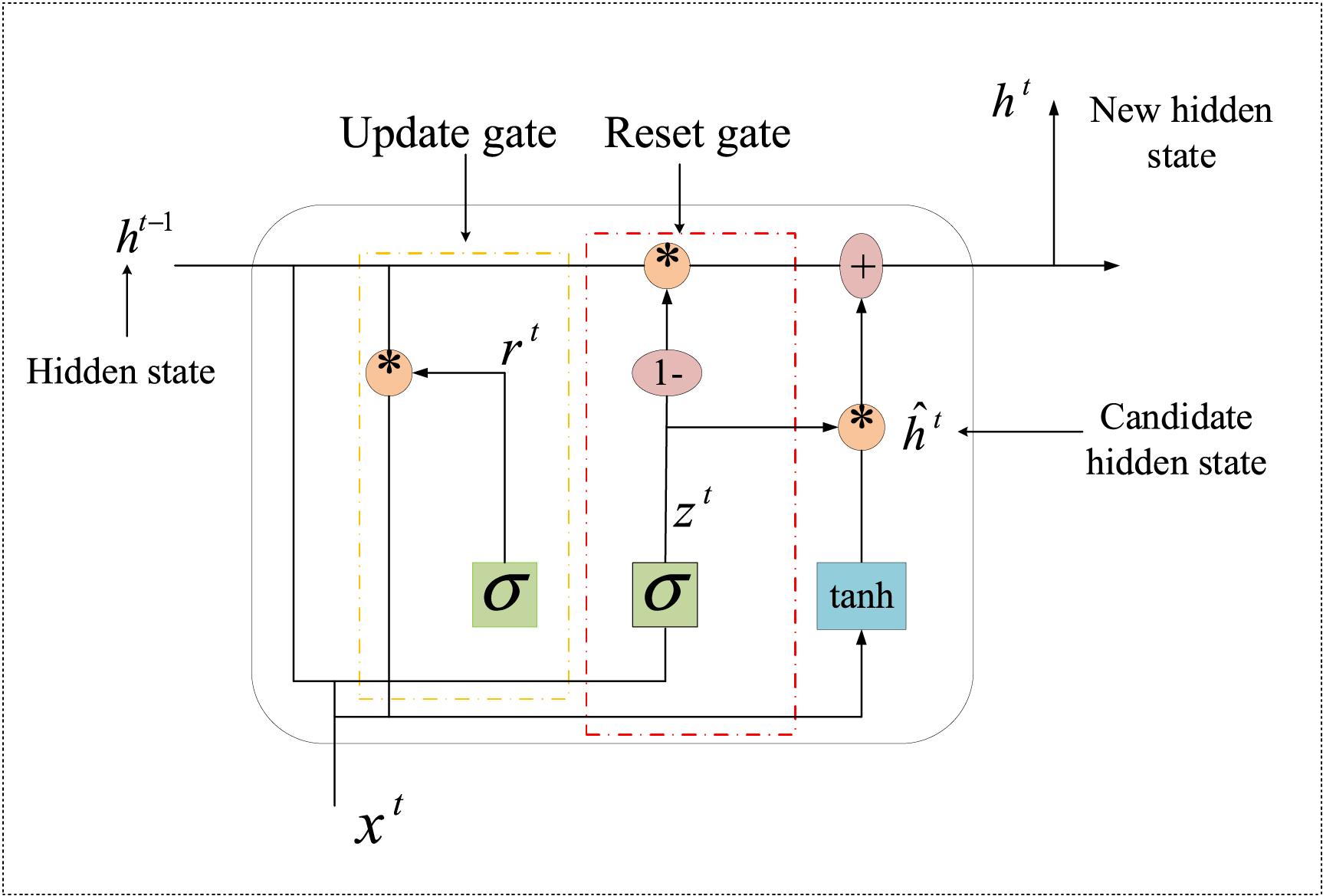
Figure 3: The architecture of GRU

The GRU cell updates its state at each time step t as follows:

Update Gate: Here, zt represents the update gate at the current time step, σ is the sigmoid activation function, and wz and bz denote the weight matrix and bias vector, respectively.

zt=σ(wzxt+wzht−1+bz)(10)

Reset Gate: Here, rt represents the reset gate at the current time step, while wr and br denote the weight matrix and bias vector, respectively.

rt=σ(wrxt+wrht−1+br)(11)

Candidate Hidden State: In this context, ⊙ denotes element-wise multiplication, and tanh represents the hyperbolic tangent activation function.

h^t=tan⁡h(wbxt+wh(rt⊙ht−1)+bh)(12)

The output state ht of the GRU is a weighted combination of the previous state ht and the candidate state h^t.

ht=zt⊙ht−1+(1−zt)⊙b^t(13)

Bidirectional GRU (BiGRU) is an extension of the standard GRU model. It consists of two independent GRU units: one forward GRU and one backward GRU. The forward GRU processes the input sequence in its original order, while the backward GRU processes the sequence in reverse order. By combining information from both directions, BiGRU is able to capture more comprehensive sequence features.

The output of BiGRU is obtained by combining the outputs of the forward and backward GRUs:

Forward GRU Output: The output generated by the forward GRU.

ht→=GRU(xt,ht−1→)(14)

Backward GRU Output: The output generated by the backward GRU.

ht←=GRU(xt,ht−1←)(15)

Final Output: The final output is obtained by performing an element-wise sum of the forward and backward GRU outputs, where ⊕ denotes the element-wise summation operation.

yt=ht→⊕ht←(16)

3  Proposed Model

In this section, we propose three multiscale CNN-BiLSTM models for addressing the multivariate classification problem of optical fiber fault diagnosis.

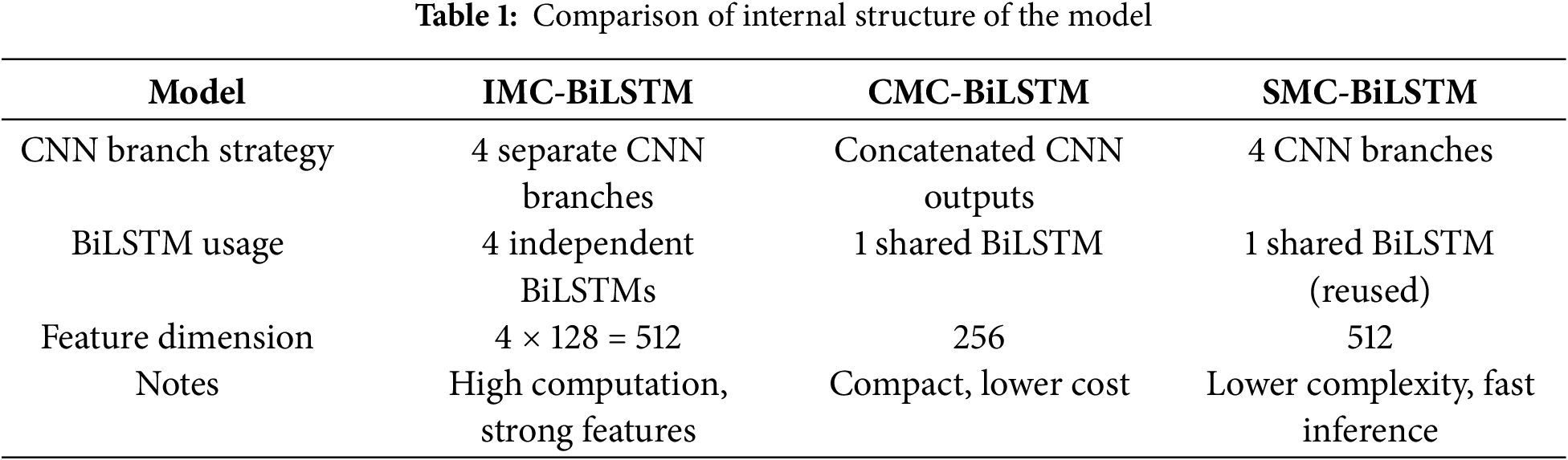
To compare different multiscale strategies, we propose three variants of a BiLSTM-based architecture: IMC-BiLSTM, CMC-BiLSTM, and SMC-BiLSTM. Each model shares a common pipeline involving convolution, sequence modeling, and classification layers, as shown in Algorithm 1. Their structural differences are summarized in Table 1. Then, we will provide a detailed description of the construction of the three proposed multi-scale CNN-BiLSTM models.

The BiLSTM used in our model follows the standard architecture introduced by Hochreiter and Schmidhuber [29], and the corresponding gate equations are provided in Section 2.1. The CNN layers are composed of 1D convolution, ReLU activation, and max-pooling operations, consistent with standard deep feature extraction practices [30]. For classification, we apply a softmax layer followed by a cross-entropy loss function to compute training gradients.

It is important to note that the proposed model is formulated as a single-label multi-class classification task, where each OTDR trace is associated with one dominant fault type (e.g., bad splice, fiber bending, or no fault). Therefore, the model predicts only one class per input sample. In real-world cases where multiple faults may co-exist along the same fiber segment, the system can still detect them by segmenting the OTDR trace and applying the model sequentially on each segment to identify distinct fault types at different locations.

3.1 IMC-BiLSTM Model

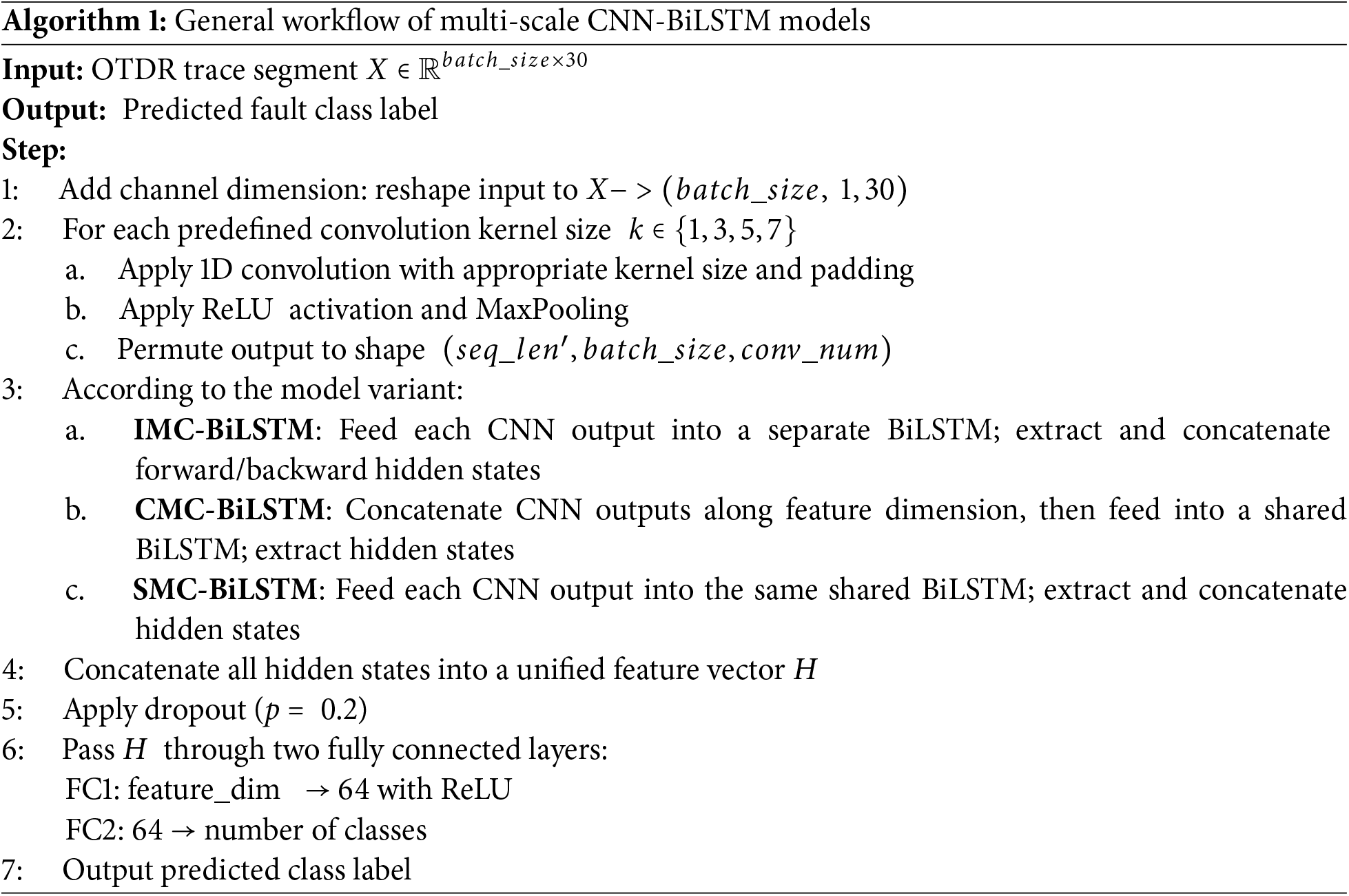
The architecture of the IMC-BiLSTM model is illustrated in Fig. 4, and its processing workflow follows Algorithm 1. In this model, the input is a sequence of 30 OTDR measurement points.

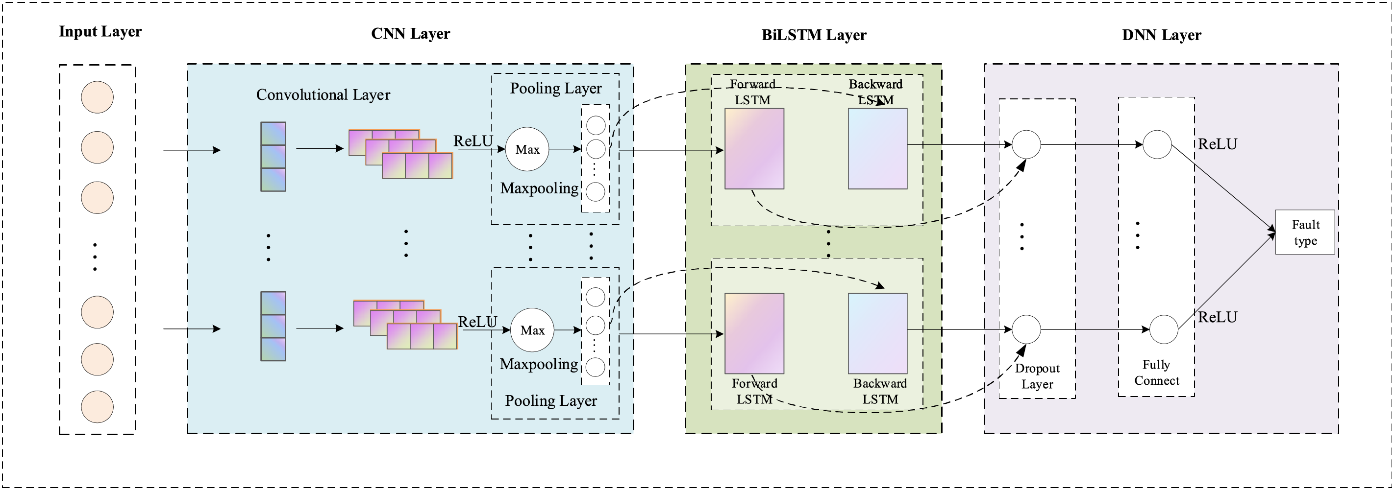
Figure 4: The architecture of IMC-BiLSTM model, where each scale of CNN is connected to an independent BiLSTM

A Multi-scale CNN module with four parallel branches (kernel sizes: 1, 3, 5, 7) is applied to extract spatial features at different scales. Each CNN branch consists of a 1D convolutional layer with 64 filters, ReLU activation, and a max-pooling operation (kernel size = 3). The outputs of these CNN branches are then processed independently by four separate BiLSTM layers, each having a hidden dimension of 64. The BiLSTM networks model the bidirectional temporal dependencies as formulated in Eqs. (7)–(9) in Section 2.2 [29].

The resulting four BiLSTM outputs are concatenated into a 512-dimensional feature vector and passed to a fully connected network with dropout and ReLU activation for classification.

3.2 CMC-BiLSTM Model

As shown in Fig. 5, the Combined Multiscale CNN-BiLSTM (CMC-BiLSTM) model reuses the multiscale CNN module from IMC-BiLSTM but applies a feature combination strategy. Instead of assigning a dedicated BiLSTM to each CNN branch, the outputs of all CNN branches are concatenated along the channel dimension and fed into a single shared BiLSTM layer for sequential modeling.

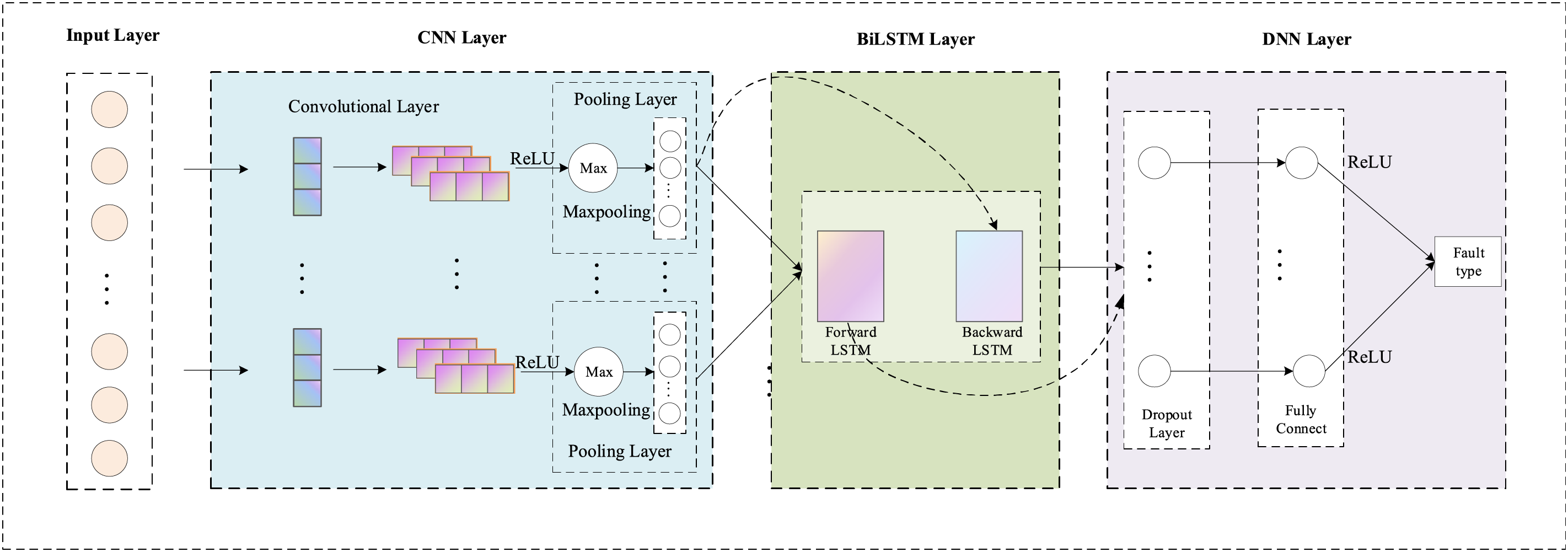
Figure 5: The architecture of the CMC-BiLSTM model, where the combination of the output of multiple scale CNN is used as the input of BiLSTM

This shared BiLSTM structure retains the ability to learn temporal dependencies while significantly reducing the number of recurrent parameters. The final BiLSTM output is passed through a two-layer dense classifier. CMC-BiLSTM achieves a good balance between representation capacity and computational cost by sharing the recurrent processing stage.

3.3 SMC-BiLSTM Model

As shown in Fig. 6. The SMC-BiLSTM model introduces further parameter sharing by applying the same BiLSTM layer sequentially to each CNN branch output. Each multiscale CNN output is processed one-by-one by the shared BiLSTM, and the resulting temporal features are concatenated into a single feature vector. This strategy minimizes the number of parameters and is especially suited for deployment in resource-constrained environments. The concatenated output is passed to a final classification layer as described in Algorithm 1. The trade-off here is reduced modeling capacity compared to IMC and CMC, but improved efficiency.

Figure 6: The architecture of SMC-BiLSTM model, where CNNs of multiple scales share an BiLSTM

4  Experiments

In this section, we conduct experiments using the publicly available OTDR_data [17] dataset and compare the proposed model with other deep learning models for optical fiber fault diagnosis.

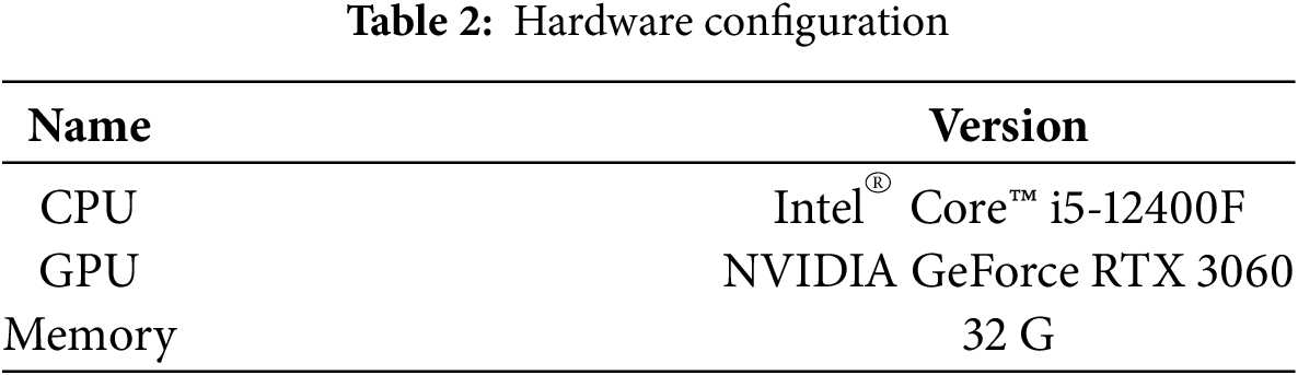
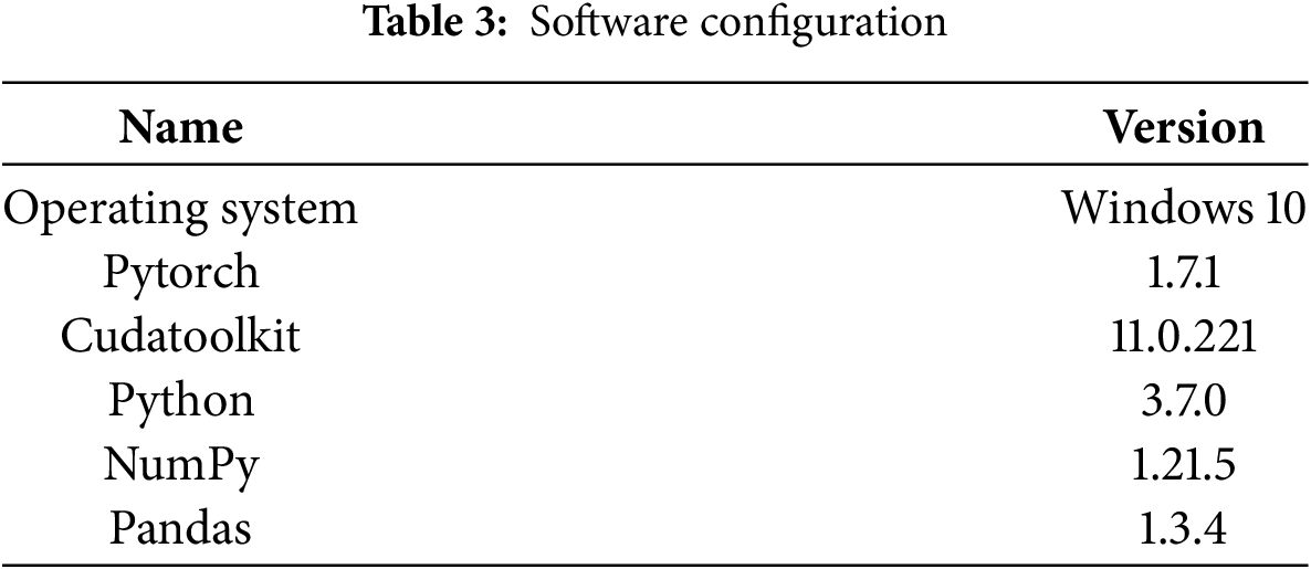
The proposed model was trained and evaluated under the hardware and software configurations shown in Tables 2 and 3.

4.1 Dataset

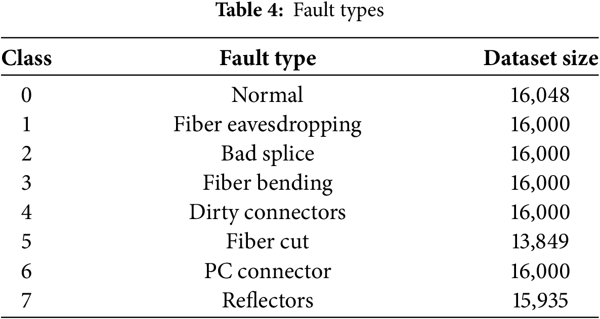
This study utilized the publicly available dataset OTDR_Data [17], which is primarily used for capturing various faults. The dataset includes six types of faults and 30 features, as shown in Table 4, Class 0 shows the normal link, class 1 to class 6 show faulty links, and class 7 shows reflectors. Overall, the dataset comprises 125,832 records. Furthermore, the collected data has already undergone a data preprocessing process.

The OTDR is configured with the following parameters: a pulse width of 10 ns, a wavelength of 1650 nm, and a sampling time of 1 ns [31]. The total length of the tested fiber optic cable is approximately 14 km.

Fig. 7 shows an example of an OTDR trace. To better illustrate the differences between fault types, we visualized the raw OTDR traces of representative samples from each class, as shown in Fig. 8. The input features consist of 30 amplitude points (P1–P30) extracted from the OTDR signal. It can be observed that different fault categories exhibit distinctive waveform patterns, such as sudden drops, gradual declines, or stable segments, which serve as important cues for classification.

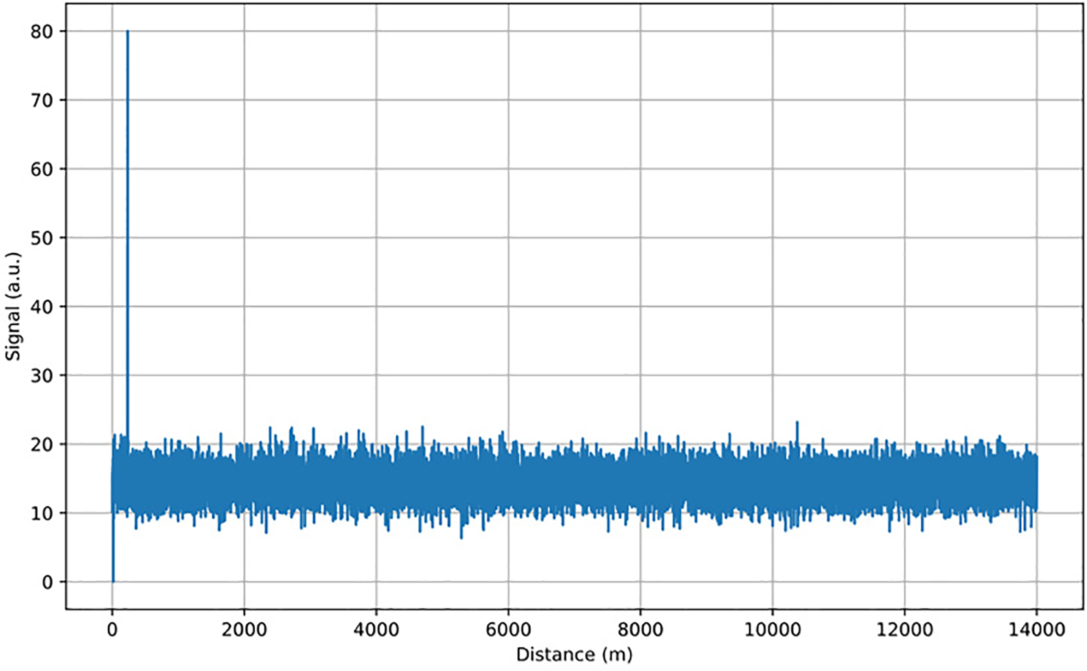
Figure 7: Example of an OTDR trace

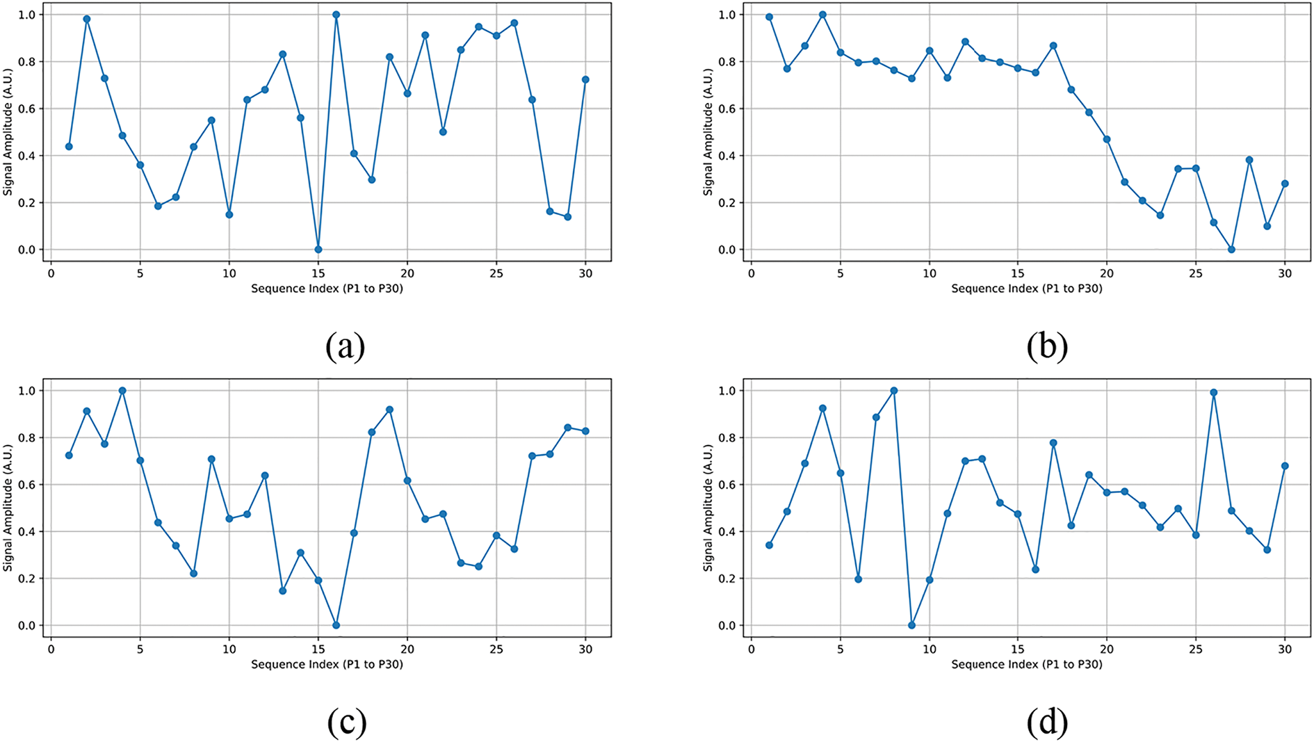
Figure 8: Representative OTDR signal trace for each class. (a) Class 0 (Normal), (b) Class 1 (fiber tapping), (c) Class 2 (bad splice), (d) Class 3 (bending event), (e) Class 4 (dirty connector), (f) Class 5 (fiber cut), (g) Class 6 (PC connector), (h) Class 7 (reflector)

4.2 Data Preprocessing

Before training the models, we performed stratified random sampling based on the dataset samples, dividing them into training, validation, and test sets in a ratio of 6:2:2. As shown in Table 5, the same training parameters were used for each model in the experiments.

4.3 Evaluation Metrics

To objectively evaluate the performance of the proposed model on the OTDR_data dataset [17] and demonstrate its advantages compared to other existing models, we employed various traditional evaluation metrics to comprehensively assess the anomaly diagnosis performance of each model. Here, TP (True Positive) represents correct predictions, TN (True Negative) represents incorrect predictions, FP represents incorrect predictions of the correct class, and FN represents incorrect predictions of the incorrect class.

Based on the above definitions, we used accuracy, precision, recall, and F1 score as classification evaluation metrics to assess the experimental results of the model.

Accuracy is the proportion of correctly classified samples out of the total number of samples. It represents the overall correctness of the model’s classification.

Acc=TP+TNTP+FP+TF+TF(17)

Precision is the proportion of true positive samples among all samples predicted as positive by the model. It reflects the model’s ability to reduce false positives.

Prc=TPTP+FP(18)

Recall is the proportion of actual positive samples that are correctly predicted as positive by the model. It indicates the model’s ability to identify all positive cases and is also known as sensitivity.

Rc=TPTP+FN(19)

The F1 score is the harmonic mean of precision and recall, providing a balanced evaluation metric that considers both false positives (FP) and false negatives (FN).

F1=2×Prc×RcPrc+Rc(20)

Delay: The fiber optics is a delay-sensitive network, which requires less delay while classifying the attack type. In the proposed system, the delay measures the average time each ML classifier takes for testing, illustrating the computational efficiency in terms of processing time. Through this evaluation, this work aims to identify classifiers that strike the optimal balance between accuracy and computational efficiency, ensuring effective fault detection while minimizing processing time.

5  Result and Analysis

5.1 Best Model Selection

As shown in Table 6, the table presents a performance comparison of various models (M1: BiGRU, M2: GRU, M3: BiLSTM, M4: LSTM) under different scale types (IMC, CMC, SMC). The specific metrics include F1-score, Precision, Recall, Accuracy, Delay (latency time), and the number of model parameters.

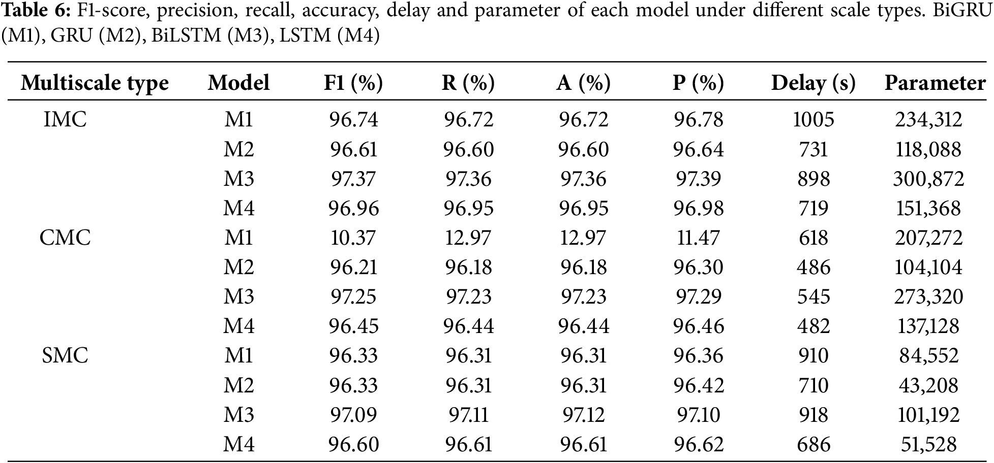
For the IMC type, M3 (BiLSTM) achieves the highest F1-score, Recall, Accuracy, and Precision, indicating its best performance under this scale type. Although M4 (LSTM) performs slightly lower than M3, the gap is minimal, and it exhibits the lowest delay (719 s) and the smallest number of parameters (151,368), making it the most efficient model. M1 (BiGRU) and M2 (GRU) perform slightly worse than M3 and M4, with longer latency times.

Under CMC type, M3 (BiLSTM) has the best performance with F1-score and Precision of 97.25% and 97.30%, which is the best performing model under this scale type. M4 (LSTM) has the lowest latency time (482 s) and the least number of parameters, which indicates that it is the most efficient, but it is slightly inferior to M3 and M2 in terms of precision. M1 (BiGRU) performance is too low compared to the other models to be informative.

For the SMC type, M3 (BiLSTM) achieves the highest F1-score, Recall, Accuracy, and Precision, all exceeding 97%, demonstrating the best performance. M4 (LSTM) shows the lowest latency (686 s) and the smallest number of parameters (51,528), making it the most efficient and suitable for scenarios requiring high real-time performance. M2 (GRU) performs close to M3 but has fewer parameters (only 43,208) and lower latency (710 s). M1 (BiGRU) exhibits the weakest performance, with an F1-score of only 96.33%, and relatively high latency and parameter counts.

Therefore, considering the overall performance metrics, M3 (BiLSTM) performs the best across all multi-scale types, achieving the highest F1 score, Precision, Recall, and Accuracy, making it suitable for scenarios demanding extremely high detection accuracy.

5.2 Optimization of Our Models

To ensure moderate complexity while achieving optimal performance, we evaluated the proposed model’s F1-score under different activation functions. Various activation functions for the hidden layers were analyzed, including Rectified Linear Unit (ReLU), Leaky ReLU, Scaled Exponential Linear Unit (SELU), Exponential Linear Unit (ELU), and Tanh. As shown in Fig. 9, using ReLU as the activation function in the hidden layers results in the highest F1 score.

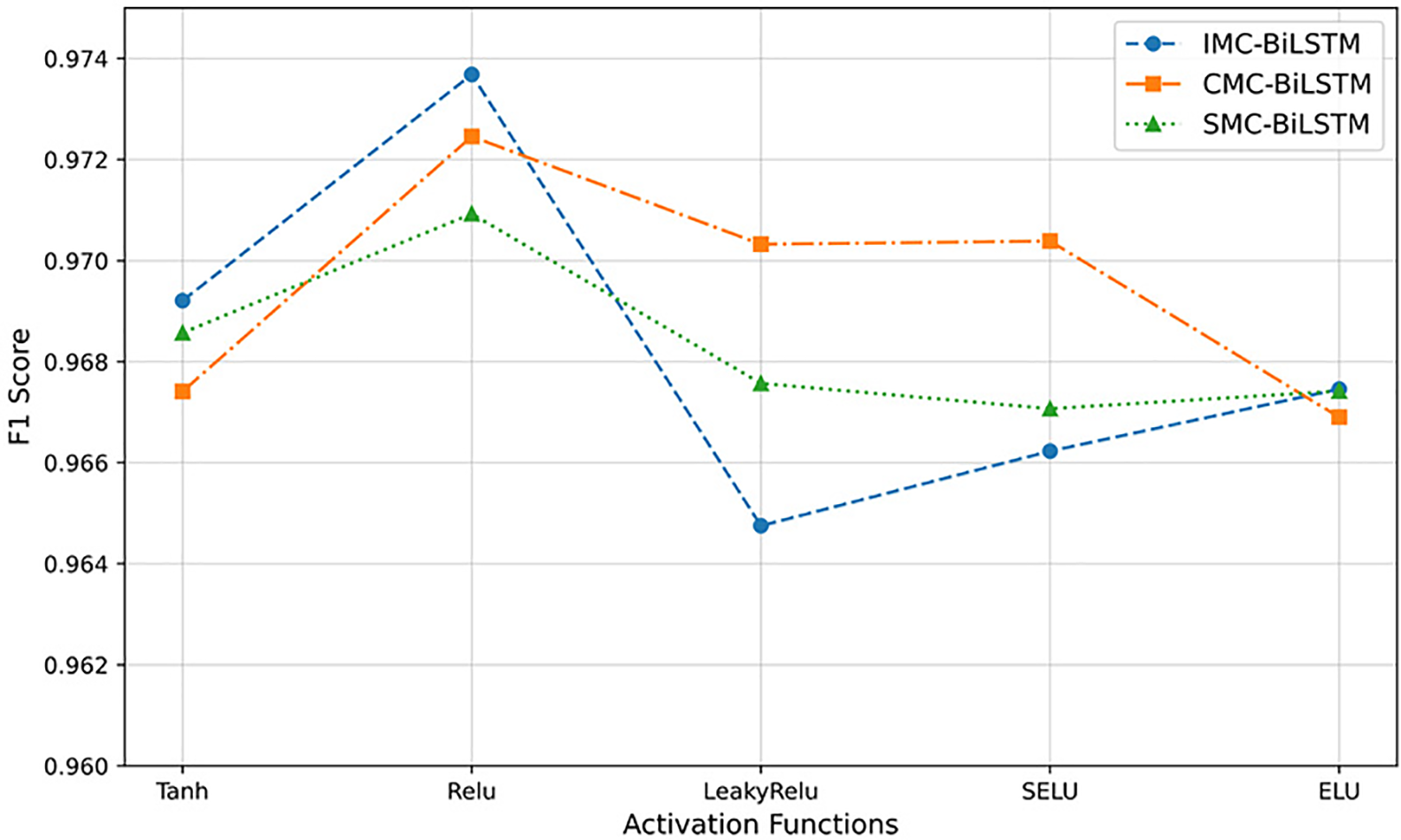
Figure 9: Average F1-scores of different activation functions over five runs

All models were trained using the Adam optimizer with an initial learning rate of 0.001, a batch size of 512, and a total of 500 training epochs. Early stopping was applied based on validation loss to prevent overfitting and improve generalization. To evaluate the impact of different activation functions on model performance, each experiment was independently repeated five times with different random seeds. The values shown in Fig. 9 represent the average F1-score computed across these five runs. Although the standard deviation is not explicitly visualized in the figure, the results remained extremely stable across all runs, with the variation in F1-score not exceeding ±0.001. This demonstrates the strong robustness and repeatability of our proposed model, regardless of initialization or data shuffling.

ReLU outperforms other activation functions due to its non-saturating behavior in the positive domain, which promotes faster convergence and more stable gradient flow during training. Unlike functions such as Tanh or SELU that may introduce vanishing gradients or internal covariate shift, ReLU provides simplicity and computational efficiency while enabling the model to better capture important features from OTDR signals. Its compatibility with deep convolutional and sequential architectures makes it especially effective for multiscale modeling tasks like fiber fault classification.

5.3 Parameter Exploration of Our Models

According to Lu et al.’s paper [16], we also discussed the parameters of the model. We conducted comparative experiments on the number of convolutional kernel types K and the number of kernels per type N to select suitable parameters. In this experiment, the max-pooling size was set to 3, and the stride M was set to 1 to balance training efficiency and the integrity of spatial features. The parameters K and N were selected from the ranges {2, 3, 4} and {16, 32, 48, 64}, respectively. Fig. 10 shows the experimental results for different parameter combinations of the three proposed models. According to the experimental results of the IMC-BiLSTM and SMC-BiLSTM models, the performance improves when both the number of convolutional kernel types and the number of kernels are large. For the CMC-BiLSTM model, the results are better when the number of kernels is 32.

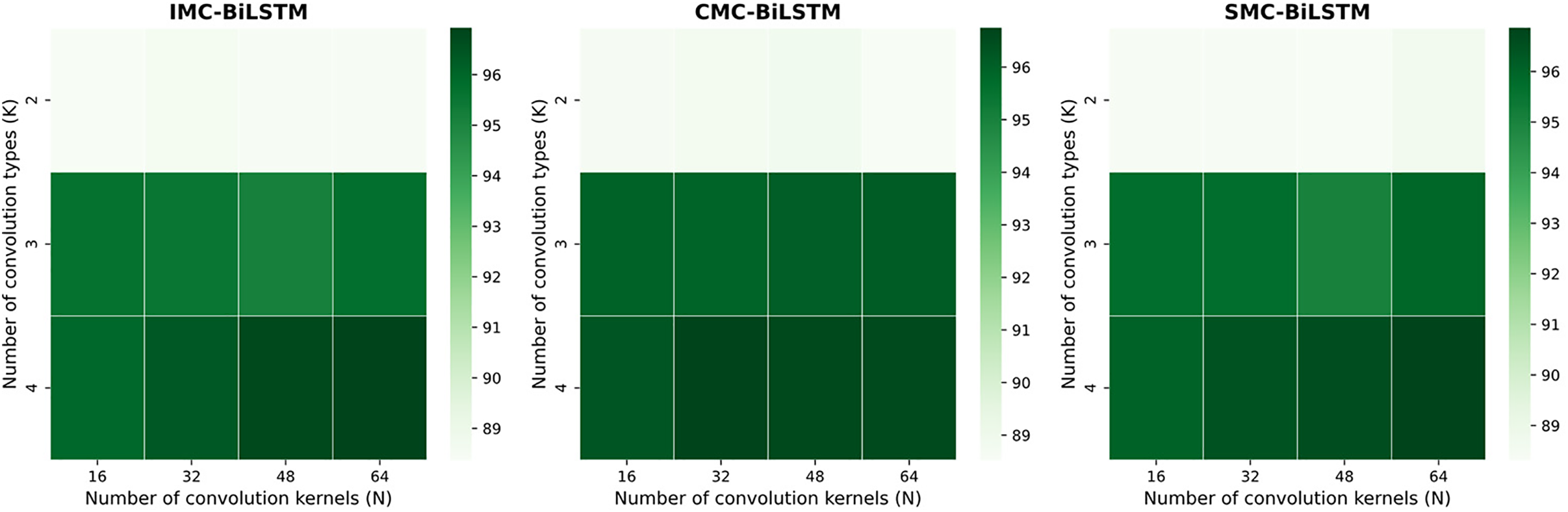
Figure 10: The F1 scores for different parameter combinations of the three proposed models. Each block represents the experimental F1 score for each parameter combination

When selecting the optimal parameter combination for each proposed model, we considered models with higher F1 scores, and when F1 scores were similar, we prioritized models with fewer parameters. Finally, the optimal parameter combinations we obtained are shown in Table 7.

5.4 Comparison of Our Model with Other Existing ML Approaches

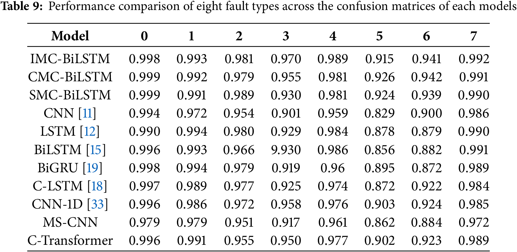
In this section, we compared the three proposed multi-scale models with existing machine learning models for optical fiber fault diagnosis found in the literature, including CNN [11], LSTM [12], BiLSTM [15], BiGRU [19], and C-LSTM [18]. To ensure a fair comparison, all these methods were tested on the same experimental dataset as the three proposed multi-scale models, and their architectures were adjusted to address only the optical fiber fault diagnosis task.

For the model architectures:

The CNN model consists of four convolutional layers, one max pooling layer, one flatten layer, one fully connected feedforward layer, followed by a dropout layer to prevent overfitting.

The LSTM model comprises a single LSTM hidden layer with 32 neurons and a fully connected layer. The BiLSTM model features one hidden layer and a fully connected layer, where the hidden layer is composed of a BiLSTM layer with 32 neurons. The BiGRU model has a similar architecture to BiLSTM, with its hidden layer consisting of a BiGRU layer with 32 units. For the C-LSTM model architecture, the CNN layers use 64 filters and convolutional kernels of size 3, while the LSTM layer employs the tanh function as the activation function for the gating mechanism. Experiments were conducted using the combined CNN-LSTM model.

In addition, we also compared our proposed models with some basic neural network models commonly used in anomaly detection, including C-LSTM-AE [32], CNN-1D [33] and Multi-scale Convolutional Neural Network (MS-CNN) and C-Transformer.

The C-LSTM-AE model, it extracts local features through two convolutional layers, captures temporal dependencies using an LSTM encoder-decoder, and performs final classification through a fully connected layer. For the structure of CNN-1D. The dimension of input data is 64, the dimension convolutional output is 12, the dimension max-pooling output is 4. The dimension of two hidden layers is 1024 and 30, respectively. The top layer is a Softmax classifier. For the structure of MS-CNN, this architecture consists of 3 channels input, 2 filter layers, 2 pooling layers and 2 fully-connected layers. For the C-Transformer model consists of two convolutional layers, each with 64 filters, followed by a Tanh activation function and a max pooling layer. The Transformer encoder utilizes a multi-head attention mechanism, and the final classification is performed using two fully connected layers.

Table 8 and Fig. 11 show that the proposed three models perform excellently in terms of F1 score, recall, accuracy, and precision. Among them, IMC-BiLSTM achieved an F1 score of 97.37%, a recall of 97.36%, an accuracy of 97.36%, and a precision of 97.39, slightly surpassing CMC-BiLSTM and SMC-BiLSTM. This indicates that IMC-BiLSTM demonstrates significant advantages in balancing performance metrics.

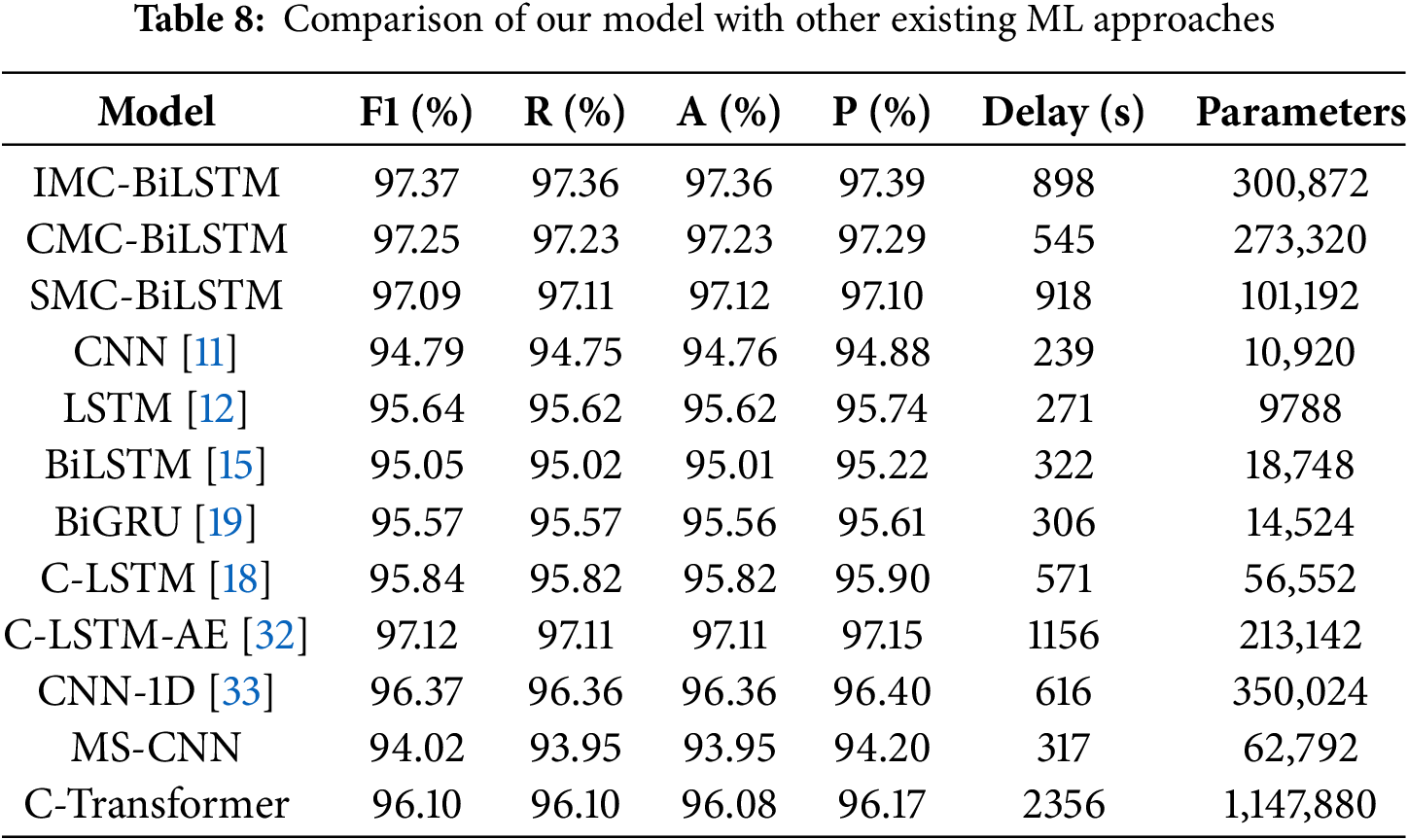
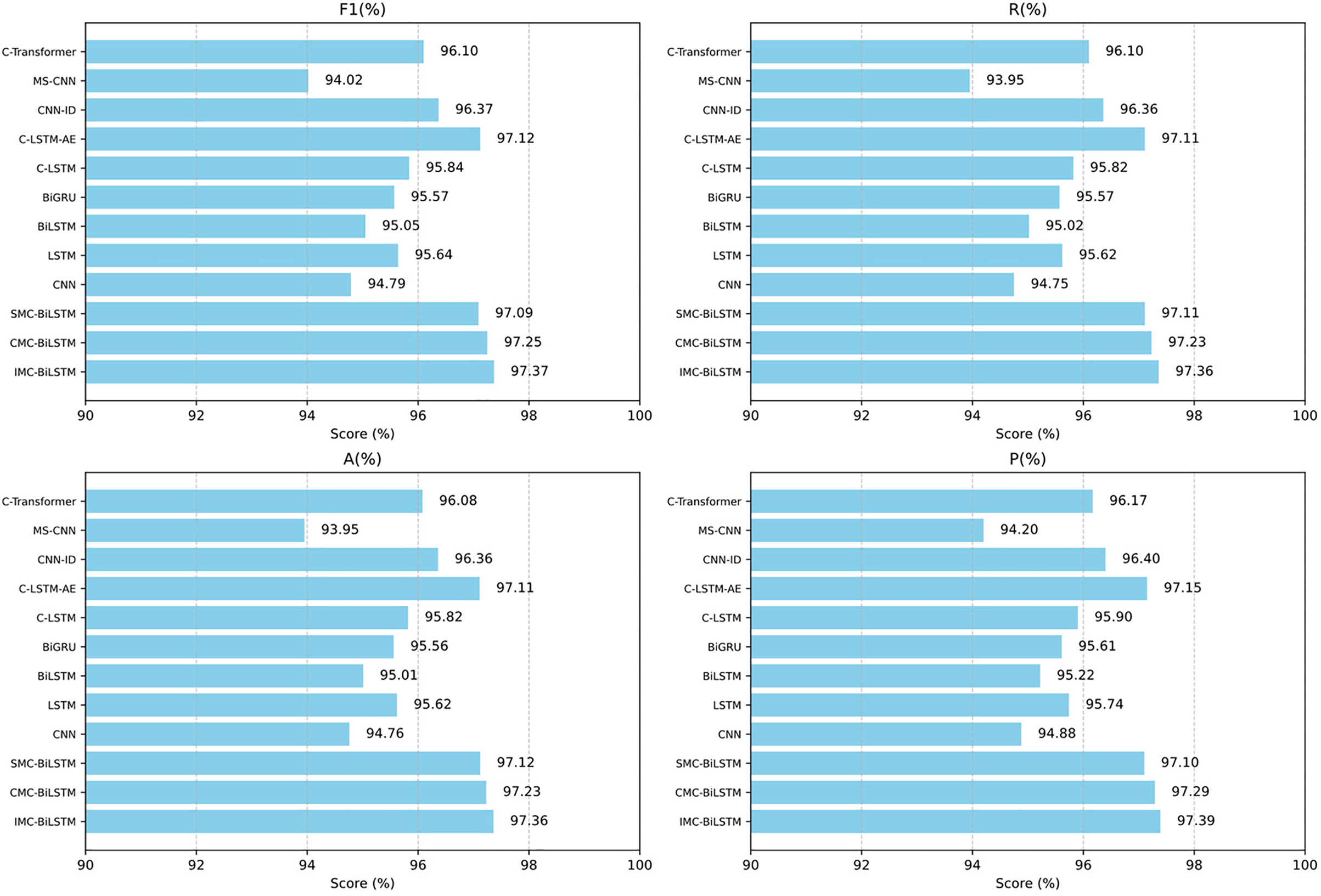
Figure 11: The scores (%) of each evaluation metric for each model. F1, R, P, and A represent the F1-score, recall, precision, and accuracy, respectively, for each model

In contrast, traditional BiLSTM and BiGRU achieved F1 scores of 95.05% and 95.57%, respectively, with accuracy scores of 95.01% and 95.56%, both significantly lower than the proposed three models. Furthermore, the performance of CNN and MS-CNN is also inferior to models like IMC-BiLSTM, with F1 scores of only 94.79% and 94.02%, respectively. Although IMC-BiLSTM exhibits the best performance, its inference delay is 898 s, which is significantly higher than other models. For example, the inference delay of CNN is only 239 s, and BiGRU’s delay is 306 s. CMC-BiLSTM shows superior performance in terms of delay, with a delay of only 545 s, which is much lower than both IMC-BiLSTM and SMC-BiLSTM. This suggests that CMC-BiLSTM achieves a better balance between high performance and lower computational cost.

In terms of the number of parameters, IMC-BiLSTM has a total of 300,872 parameters, while CMC-BiLSTM and SMC-BiLSTM have 273,320 and 101,192 parameters, respectively. Although the number of parameters is relatively high, compared to other complex models (such as C-Transformer, which has 1,147,880 parameters), the proposed three models strike a good balance between performance and model complexity.

Overall, the proposed three models (IMC-BiLSTM, CMC-BiLSTM, and SMC-BiLSTM) outperform existing models in key performance metrics (F1, Recall, Accuracy, Precision), especially IMC-BiLSTM, which achieved an F1 score of 97.37%, significantly higher than traditional models (e.g., BiLSTM and CNN). Although IMC-BiLSTM has a higher inference delay, CMC-BiLSTM achieves a better balance between performance and delay through appropriate optimization, making it a more practical choice. In comparison, the parameter size advantage of SMC-BiLSTM makes it suitable for resource-constrained scenarios.

5.5 Fault Diagnosis Capability

As previously mentioned, after performance optimization, we selected the optimal model by analyzing the F1-score of three models (IMC-BiLSTM, CMC-BiLSTM, and SMC-BiLSTM) under different activation functions. All three models were trained using datasets containing both normal and faulty data to model different fault types. Once trained, the three models can distinguish between normal states and different types of faults in terms of the average precision metric. Additionally, we compared the confusion matrices of a total of each models, as shown in Fig. 12 and Table 9.

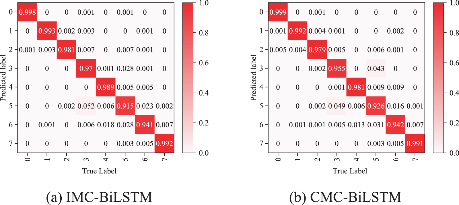
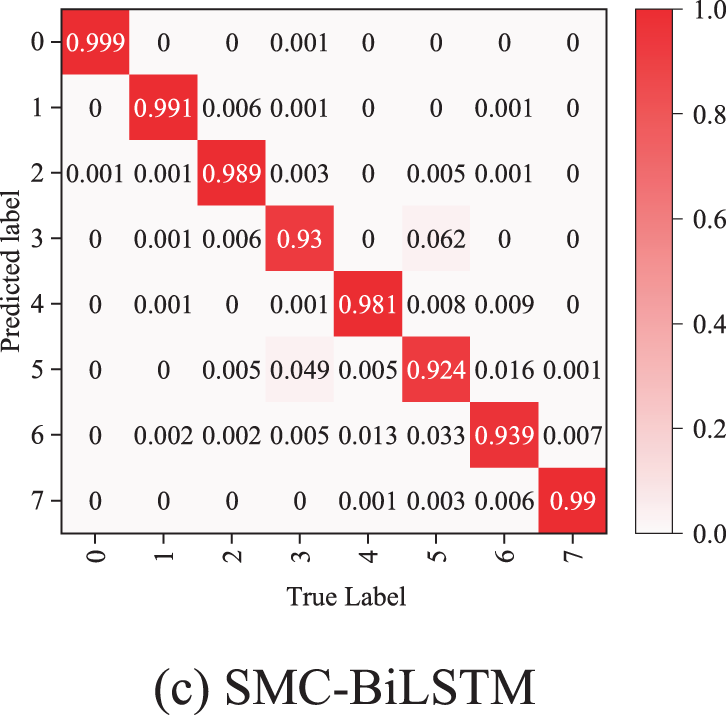
Figure 12: Confusion matrix comparisons of three Models. (a) IMC-BiLSTM (b) CMC-BiLSTM (c) SMC-BiLSTM. Class 0 (Normal), Class 1 (fiber tapping), Class 2 (bad splice), Class 3 (bending event), Class 4 (dirty connector), Class 5 (fiber cut), Class 6 (PC connector), Class 7 (reflector)

As shown in Fig. 12a, the IMC-BiLSTM model achieves an accuracy of over 97% in classifying three types of faults: fiber eavesdropping (Class 1), bad splice (Class 2), bending event (Class 3) and dirty connectors (Class 4), demonstrating robust classification capability. In particular, for diagnosing fiber eavesdropping (Class 1), the accuracy reaches 99.3%, indicating that the model is highly effective in capturing the features of this type of fault. For faults with more distinct features or better separability (such as dirty connectors and fiber eavesdropping), the IMC-BiLSTM model can accurately identify them through its built-in feature extraction and classification capabilities.

As shown in Fig. 12b, the CMC-BiLSTM model demonstrates certain improvements in overall performance compared to the IMC-BiLSTM model, particularly in classifying fiber eavesdropping, poor splicing, and dirty connectors, with classification accuracy still exceeding 97%. For fiber cut, the classification accuracy reaches 92.6%, a 1.1% increase compared to the IMC-BiLSTM model, further proving the model’s strong detection capability for this type of fault. In terms of feature extraction generalization, the CMC-BiLSTM model may be more suitable for classifying different fault modes. Overall, the CMC-BiLSTM model outperforms the IMC-BiLSTM model in classification accuracy, particularly excelling in diagnosing fiber eavesdropping faults.

As shown in Fig. 12c, compared to the first two models, SMC-BiLSTM performs relatively poorly in overall classification accuracy, particularly in the classification task of bending events (Class 3), where the accuracy decreases significantly compared to IMC-BiLSTM and CMC-BiLSTM. For fiber eavesdropping (Class 1), the accuracy remains at 99.1%, which is essentially consistent with IMC-BiLSTM and CMC-BiLSTM. This model demonstrates stronger adaptability and representation capabilities for certain types of fault features, such as bad splices, with an accuracy improvement of 0.8% and 1% compared to IMC-BiLSTM and CMC-BiLSTM, respectively.

In addition, the comparison of the confusion matrices of the proposed three models with the other models, as shown in Table 9, clearly shows that the proposed methods have better diagnostic consistency in general. Especially in fiber cut (Class 5) and PC connector (Class 6), the performance of the proposed three models is improved by about 1.2%–10% on fiber cut (Class 5) and 1.5%–7% on PC connector (Class 6) compared to other models.

In summary, the proposed three models provide strong evidence of their effectiveness and superiority in optical fiber fault diagnosis. The experimental results demonstrate that these methods are highly capable of diagnosing optical fiber faults, with significant practical implications, highlighting their generality and reliability in real-world fault diagnosis scenarios.

The ROC quoted in Fig. 13 show that our model can distinguish between different event causes. The overall AUC (Area Under the Curve) performance of the model is high and its classification ability is balanced across categories, indicating its suitability for this multi-classification task.

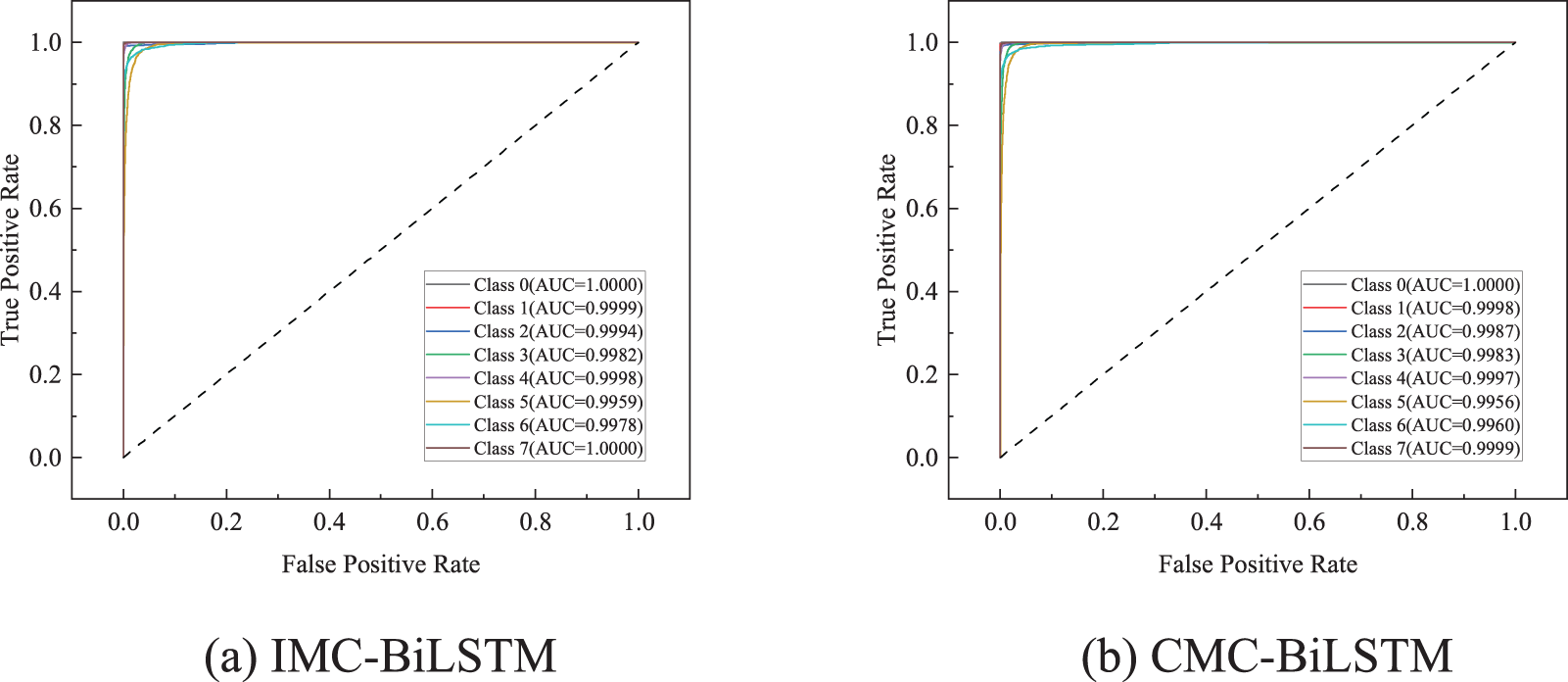
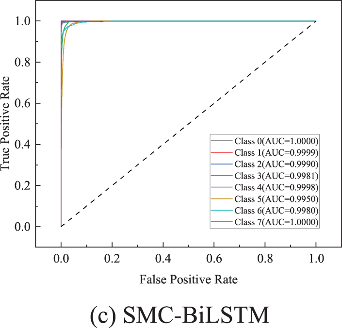
Figure 13: ROC curves for the three models. (a) IMC-BiLSTM (b) CMC-BiLSTM (c) SMC-BiLSTM. Class 0 (Normal), Class 1 (fiber tapping), Class 2 (bad splice), Class 3 (bending event), Class 4 (dirty connector), Class 5 (fiber cut), Class 6 (PC connector), Class 7 (reflector)

To observe the event distinguishability of the proposed three methods, the t-distributed Stochastic Neighbor Embedding (t-SNE) technique [34] was employed to visually study the feature learning capabilities of the three models (IMC-BiLSTM, CMC-BiLSTM, and SMC-BiLSTM) on OTDR fault data. As shown in Fig. 14. From the first three figures, it can be observed that the proposed three methods can effectively distinguish the visual features of the 8 events, demonstrating that all three methods achieved optimal performance in this test. In contrast, the last figure shows that the CNN model exhibits relatively poor distinguishability for the 8 events. Furthermore, the proposed three models demonstrate the ability to learn effective features for accurate fault diagnosis.

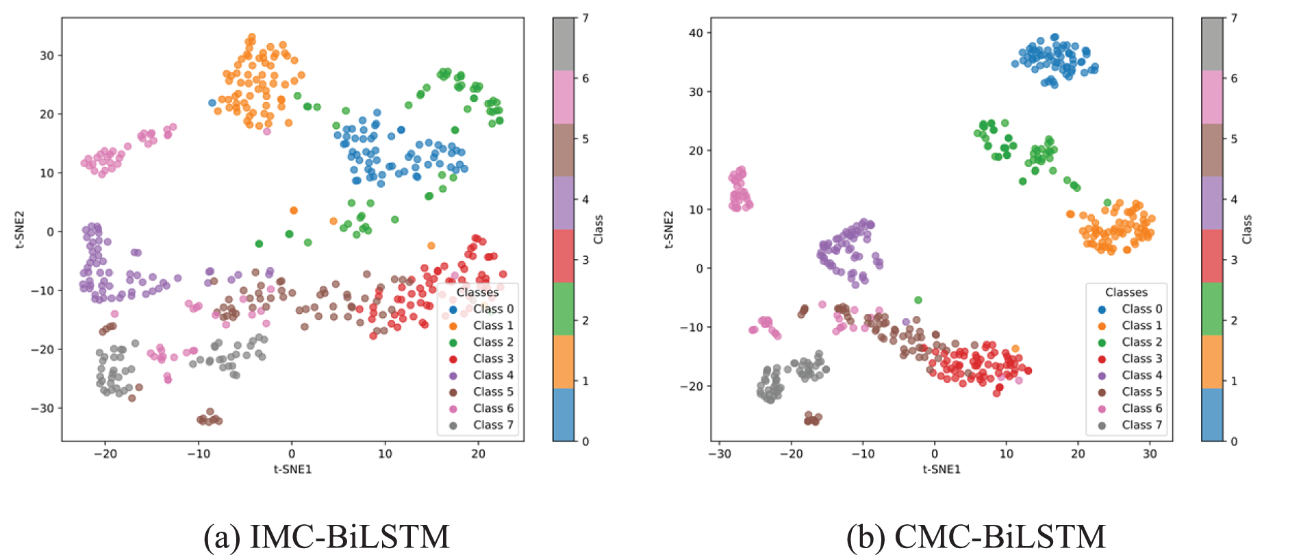
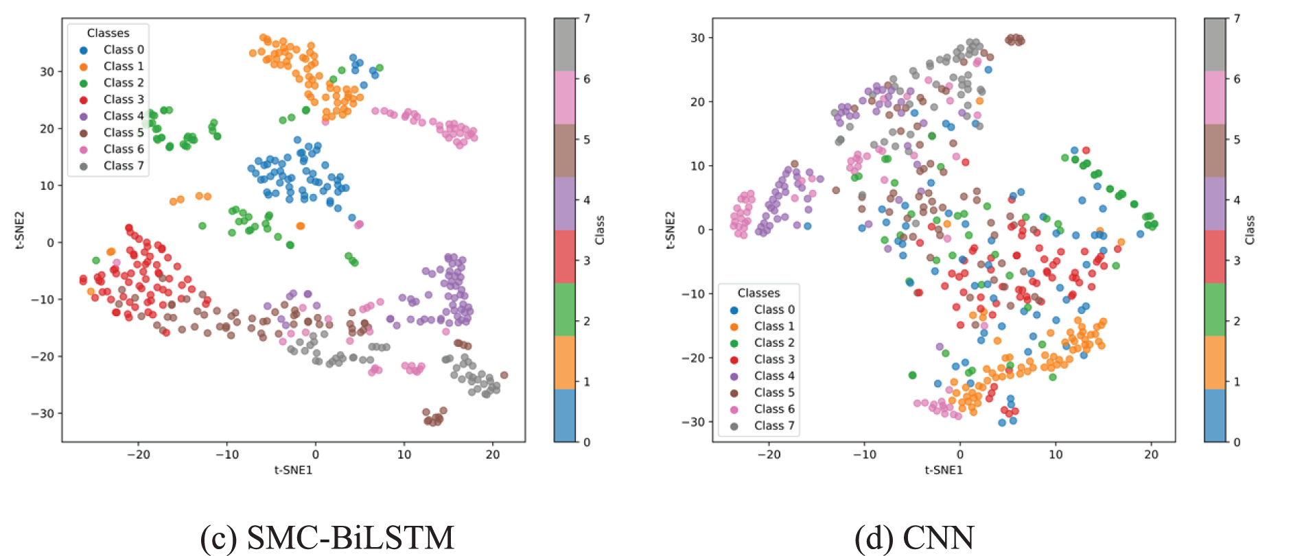
Figure 14: Visualization of feature learning under different models. (a) IMC-BiLSTM (b) CMC-BiLSTM (c) SMC-BiLSTM (d) CNN

6  Conclusions

To address the limitations in sequential spatial feature extraction of OTDR fiber data, we proposed a multiscale CNN-BiLSTM framework. This framework replaces fixed-size convolutional kernels with multiscale kernels of varying sizes, enabling better handling of OTDR data for fiber fault diagnosis. Experimental results demonstrate that our three proposed models (IMC-BiLSTM, CMC-BiLSTM, and SMC-BiLSTM) outperform existing models in key performance metrics such as F1-score and accuracy. In particular, IMC-BiLSTM achieved an F1-score of 97.37%, significantly surpassing traditional models like BiLSTM and CNN. Although IMC-BiLSTM exhibits higher inference latency, CMC-BiLSTM offers a more practical balance between performance and delay, while SMC-BiLSTM shows advantages in parameter efficiency, making it suitable for resource-constrained environments. In future work, we plan to explore lightweight architectures to reduce inference time and model complexity. We also aim to incorporate self-supervised or semi-supervised learning strategies to alleviate reliance on large labeled datasets. Additionally, we will investigate expanding the model’s capability to detect and localize multiple co-existing faults within a single OTDR trace, further enhancing its practicality in real-world fiber monitoring scenarios.

Acknowledgement: The authors acknowledge the support received from the Guangxi Science and Technology Department Key Research and Development Project, the Guangxi Key Research and Development Plan Project and Guangxi Key Laboratory of Embedded Technology and Intelligent System.

Funding Statement: This work was supported in part by the Guangxi Science and Technology Department Key Research and Development Project (Grant No. 23026149); in part by the Guangxi Key Research and Development Plan Project (Grant No. AB24010073).

Author Contributions: Jinku Qiu: Writing—review & editing, Writing—original draft, Visualization, Validation, Software, Methodology, Investigation, Formal analysis, Data curation, Conceptualization; Xiaoping Yang: Writing—review & editing, Resources, Fund acquisition; Xifa Gong and Jin Ye: Supervision, Fund acquisition; Fei Yao: Project administration, Conceptualization, Fund acquisition; Jiaqiao Chen, Xianzan Luo and Da Qin: Review, Fund acquisition. All authors reviewed the results and approved the final version of the manuscript.

Availability of Data and Materials: All data generated or analyzed during this study are included in this published article.

Ethics Approval: Not applicable.

Conflicts of Interest: The authors declare no conflicts of interest to report regarding the present study.

References

1. The Fiber Optic Association, Inc., Optical Time Domain Reflectometer (OTDRThe Fiber Optic Association, Inc., 2013 [Internet]. [cited 2025 Apr 24]. Available from: https://www.thefoa.org/tech/ref/testing/OTDR/OTDR.html. [Google Scholar]

2. Liu F, Zarowski CJ. Events in fiber optics given noisy OTDR data. I. GSR/MDL method. IEEE Trans Instrum Meas. 2001;50(1):47–58. doi:10.1109/19.903877. [Google Scholar] [CrossRef]

3. Liu F, Zarowski CJ. Detection and location of connection splice events in fiber optics given noisy OTDR data. Part II. R1MSDE method. IEEE Trans Instrum Meas. 2004;53(2):546–56. doi:10.1109/TIM.2003.820442. [Google Scholar] [CrossRef]

4. Man X, Dong Y, He H, Hu W. Analysis of connection splice events in OTDR data using short Fourier transform method. Yi Qi Yi Biao Xue Bao/Chin J Sci Instrum. 2010;31(9):2121–5. [Google Scholar]

5. Zhang X, Zhao H, Sun G, Cui T. Localization of non-reflective events in OTDR data combining DWT with template matching. In: 2011 4th International Congress on Image and Signal Processing; 2011 Oct 15–17; Shanghai, China. 2011. Vol. 4, p. 2275–9. doi:10.1109/CISP.2011.6100609. [Google Scholar] [CrossRef]

6. Gu X, Sablatash M. Estimation and detection in OTDR using analyzing wavelets. In: Proceedings of IEEE-SP International Symposium on Time-Frequency and Time-Scale Analysis; 1994 Oct 25–28; Philadelphia, PA, USA. p. 353–6. doi:10.1109/TFSA.1994.467337. [Google Scholar] [CrossRef]

7. Kong H, Dong Y, Zhou Q, Xie W, Ma C, Hu W. Events detection in OTDR data based on a method combining correlation matching with STFT. In: Asia Communications and Photonics Conference; 2014 Nov 11–14; Shanghai, China. doi:10.1364/ACPC.2014.ATh3A.148. [Google Scholar] [CrossRef]

8. Abdelli K, Rafique D, Pachnicke S. Machine learning based laser failure mode detection. In: 2019 21st International Conference on Transparent Optical Networks (ICTON); 2019 Jul 9–13; Angers, France. p. 1–4. doi:10.1109/ICTON.2019.8840267. [Google Scholar] [CrossRef]

9. Abdelli K, Rafique D, Grießer H, Pachnicke S. Lifetime prediction of 1550 nm DFB laser using machine learning techniques. In: Optical Fiber Communication Conference. Washington, DC, USA: Optica Publishing Group; 2020. doi:10.1364/OFC.2020.Th2A.3. [Google Scholar] [CrossRef]

10. Abdelli K, Grießer H, Pachnicke S. Machine learning based data driven diagnostic and prognostic approach for laser reliability enhancement. In: 2020 22nd International Conference on Transparent Optical Networks (ICTON); 2020 Jul 19–23; Bari, Italy. p. 1–4. doi:10.1109/ICTON51198.2020.9203551. [Google Scholar] [CrossRef]

11. Abdelli K, Griesser H, Pachnicke S. Convolutional neural networks for reflective event detection and characterization in fiber optical links given noisy OTDR signals. In: Photonic Networks; 22th ITG Symposium; 2021 May 19–20; Online. p. 1–5. doi:10.48550/arXiv.2203.14820. [Google Scholar] [CrossRef]

12. Abdelli K, Grießer H, Ehrle P, Tropschug C, Pachnicke S. Reflective fiber fault detection and characterization using long short-term memory. J Opt Commun Netw. 2021;13(10):E32–41. doi:10.1364/JOCN.423625. [Google Scholar] [CrossRef]

13. Zhang W, Li C, Peng G, Chen Y, Zhang Z. A deep convolutional neural network with new training methods for bearing fault diagnosis under noisy environment and different working load. Mech Syst Signal Process. 2018;100(6):439–53. doi:10.1016/j.ymssp.2017.06.022. [Google Scholar] [CrossRef]

14. Abdelli K, Grießer H, Tropschug C, Pachnicke S. A BiLSTM-CNN based multitask learning approach for fiber fault diagnosis. In: Optical Fiber Communication Conference. Washington, DC, USA: Optica Publishing Group; 2021. doi:10.1364/OFC.2021.M3C.7. [Google Scholar] [CrossRef]

15. Abdelli K, Grießer H, Tropschug C, Pachnicke S. Optical fiber fault detection and localization in a noisy OTDR trace based on denoising convolutional autoencoder and bidirectional long short-term memory. J Lightwave Technol. 2022;40(8):2254–64. doi:10.1109/JLT.2021.3138268. [Google Scholar] [CrossRef]

16. Lu YX, Jin XB, Liu DJ, Zhang XC, Geng GG. Anomaly detection using multiscale C-LSTM for univariate time-series. Secur Commun Netw. 2023;2023(1):6597623. doi:10.1155/2023/6597623. [Google Scholar] [CrossRef]

17. Abdelli K, Azendorf F, Tropschug C, Griesser H, Pachnicke S, Choo J. Dataset for optical fiber faults. IEEE Dataport. 2022. doi:10.21227/pdpn-1b78. [Google Scholar] [CrossRef]

18. Soothar KK, Chen Y, Magsi AH, Hu C, Shah H. Optimizing optical fiber faults detection: a comparative analysis of advanced machine learning approaches. Comput Mater Contin. 2024;79(2):2697–721. doi:10.32604/cmc.2024.049607. [Google Scholar] [CrossRef]

19. Prakash P, Kasthuri P. Machine learning based denoising anomaly detection and localisation using BiGRU in optical fiber monitoring. In: 2024 First International Conference on Electronics, Communication and Signal Processing (ICECSP); 2024 Aug 8–10; New Delhi, India. p. 1–5. doi:10.1109/ICECSP61809.2024.10698456. [Google Scholar] [CrossRef]

20. Xu C, Liang R, Wu X, Cao C, Chen J, Yang C, et al. A hybrid model integrating CNN-BiLSTM and CBAM for anchor damage events recognition of submarine cables. IEEE Trans Instrum Meas. 2023;72:1–11. doi:10.1109/TIM.2023.3290323. [Google Scholar] [CrossRef]

21. Zheng X, Tang R, Wang J, Lin C, Chen J, Wang N, et al. Research on multi-source simultaneous recognition technology based on Sagnac fiber optic sound sensing system. Photonics. 2023;10(9):1003. doi:10.3390/photonics10091003. [Google Scholar] [CrossRef]

22. Wu H, Chen J, Liu X, Xiao Y, Wang M, Zheng Y, et al. One-dimensional cnn-based intelligent recognition of vibrations in pipeline monitoring with DAS. J Lightwave Technol. 2019;37(17):4359–66. doi:10.1109/JLT.2019.2923839. [Google Scholar] [CrossRef]

23. Zhou C, Sun C, Liu Z, Lau F. A C-LSTM neural network for text classification. arXiv:1511.08630. 2015. doi:10.48550/arXiv.1511.08630. [Google Scholar] [CrossRef]

24. Chua LO. CNN: a vision of complexity. Int J Bifurcat Chaos. 1997;7(10):2219–425. doi:10.1142/S0218127497001618. [Google Scholar] [CrossRef]

25. Greff K, Srivastava RK, Koutník J, Steunebrink BR, Schmidhuber J. LSTM: a search space odyssey. IEEE Trans Neural Netw Learn Syst. 2016;28(10):2222–32. doi:10.1109/TNNLS.2016.2582924. [Google Scholar] [PubMed] [CrossRef]

26. Siami-Namini S, Tavakoli N, Namin AS. The performance of LSTM and BiLSTM in forecasting time series. In: 2019 IEEE International Conference on Big Data (Big Data); 2019 Dec 9–12; Los Angeles, CA, USA. p. 3285–92. doi:10.1109/BigData47090.2019.9005997. [Google Scholar] [CrossRef]

27. Dey R, Salem FM. Gate-variants of gated recurrent unit (GRU) neural networks. In: IEEE 60th International Midwest Symposium on Circuits and Systems (MWSCAS); 2017 Aug 6–9; Medford, MA, USA. p. 1597–600. doi:10.1109/MWSCAS.2017.8053243. [Google Scholar] [CrossRef]

28. Cho K, Van Merriënboer B, Gulcehre C, Bahdanau D, Bougares F, Schwenk H, et al. Learning phrase representations using RNN encoder-decoder for statistical machine translation. arXiv:1406.1078. 2014. doi 10.48550/arXiv.1406.1078. [Google Scholar] [CrossRef]

29. Hochreiter S, Schmidhuber J. Long short-term memory. Neural Comput. 1997;9(8):1735–80. doi:10.1162/neco.1997.9.8.1735. [Google Scholar] [PubMed] [CrossRef]

30. LeCun Y, Bottou L, Bengio Y, Haffner P. Gradient-based learning applied to document recognition. Proc IEEE. 2002;86(11):2278–324. doi:10.1109/5.726791. [Google Scholar] [CrossRef]

31. Abdelli K, Cho JY, Azendorf F, Griesser H, Tropschug C, Pachnicke S. Machine-learning-based anomaly detection in optical fiber monitoring. J Opt Commun Netw. 2022;14(5):365–75. doi:10.1364/JOCN.451289. [Google Scholar] [CrossRef]

32. Yin C, Zhang S, Wang J, Xiong NN. Anomaly detection based on convolutional recurrent autoencoder for IoT time series. IEEE Trans Syst Man Cybern Syst. 2020;52(1):112–22. doi:10.1109/TSMC.2020.2968516. [Google Scholar] [CrossRef]

33. Zeng M, Nguyen LT, Yu B, Mengshoel OJ, Zhu J, Wu P, et al. Convolutional neural networks for human activity recognition using mobile sensors. In: 6th International Conference on Mobile Computing, Applications and Services; 2014 Nov 6–7; Austin, TX, USA. p. 197–205. doi:10.4108/icst.mobicase.2014.257786. [Google Scholar] [CrossRef]

34. Van der Maaten L, Hinton G. Visualizing data using t-SNE. J Mach Learn Res. 2008;9(11):2579–605. [Google Scholar]