Leveraging Machine Learning to Predict Hospital Porter Task Completion Time

1  Introduction

Porters play a critical role in ensuring smooth hospital operations. Their primary responsibility is to ensure the efficient transportation of vital medical items, like lab specimens, reports, and blood products, and to safely transport patients throughout the facility. This role is essential for maintaining high-quality patient care and coordinating various departments. Any delays or disruptions in porter services can significantly slow down the overall workflow and impact timely care delivery [1,2]. For example, delays in transporting lab results or blood can cause problems for doctors who need this information to make quick decisions about patient care. Similarly, delays in transferring patients can cause longer waits and increase risks. It’s important to make sure patients get to their destinations on time [3]. A major challenge hospitals face is a lack of transparency around estimated arrival and completion times for porter tasks. Without this information, staffs cannot accurately predict when items will arrive or tasks will be completed. This makes it extremely difficult to properly allocate resources and manage time effectively. Therefore, by providing staff with reliable predictions of porter tasks, hospitals can optimize their workflows, reduce unnecessary delays, and enhance overall hospital efficiency.

Numerous studies in the field of healthcare information have focused on improving medical efficiency and enhancing overall operational effectiveness. Predicting patient waiting times has been a widely studied area. Chen et al. [4] addressed the patient waiting times problem in overcrowded hospitals. They developed a modified version of Random Forest (RF) for predicting wait times based on user characteristics and presented results through a mobile app. To handle real-time computation of large-scale datasets, their computations were performed on a cloud-based platform. However, there is a lack of performance comparison with commonly used tree-based algorithms, such as Gradient Boosting Machines or Decision Trees, limiting their assessment and applicability. Robbani and Ullah [5] conducted research to predict the length of hospital stay for COVID-19 patients, aiming to optimize resource allocation and improve patient care. To handle the challenge of imbalanced data, they employed synthetic minority oversampling technique in their machine learning approach. In their experiments, K-Nearest Neighbors (KNN), Random Forest (RF), Decision Tree (DT), and Gradient Boosting (GB) were adopted for performance comparison. However, predicting length of stay is a regression task, requiring the estimation of a continuous duration, not categories. Treating it as a classification problem might overlook important factors in predicting stays, leading to less accurate results.

In this work, we utilize machine learning-based approaches to predict the completion time of porter tasks. For this, we first identified key features that can impact porter tasks. We then evaluated three different machine learning algorithms. Finally, we used ensemble modeling to aggregate the predictions of each algorithm. To our best knowledge, this is the first work that explores the problem of predicting porter delivery time. The major contributions of this work are described as follows:

1. We conducted a detailed analysis to examine the impact of feature selection methods on model performance. To accomplish this, we first performed a comprehensive preprocessing stage. We then evaluated the effectiveness of filter methods, wrapper methods, and embedded methods in optimizing machine learning models. Please refer to Section 3 for details.

2. We compared three different tree-based algorithms, including decision trees (DT), random forests (RF), and gradient boosting (GB), for prediction. To maximize the performance of the model, we conducted hyperparameter tuning. Additionally, a grid search was performed to determine the optimal weights among all the models for training an ensemble model (EM). A detailed discussion of these algorithms can be found in Section 4.

3. The proposed EM method outperforms DT, RF, and GB models in predicting porter task completion times. It achieves a mean absolute error of 3 min in predicting task response time and 4.42 min in task completion time. In particular, the prediction error of the EM is 52.1% lower compared to using only the historical average for predicting task response time, and 46.55% lower for task completion time. The ensemble modeling technique significantly improves accuracy in estimating porter task duration. Please refer to Section 5 for details.

In summary, our method simplifies hospital transportation, benefiting patients, ward staff, and porter managers. For patients, it reduces waiting times, improving their overall healthcare experience. Ward staff can optimize workflow by minimizing unnecessary wait times for porters. Porter managers gain valuable insights to better manage transportation tasks efficiently. The paper is organized as follows: Section 2 reviews related literature, Section 3 presents data analysis, Section 4 introduces the models, Section 5 compares experimental results, and Section 6 concludes the work.

2  Related Work

2.1 Cross-Domain Applications for Task Time Prediction

Machine learning techniques have been applied across various industries to predict task completion times, demonstrating their versatility and cross-domain potential. In logistics, they have been used to forecast order volumes and staffing needs, enabling optimized resource allocation and improved operational efficiency [6]. Similarly, in manufacturing, neural networks have helped predict machining cycle times, supporting better production planning and reduced lead times [7]. In customer service logistics, artificial intelligence-driven (AI-driven) platforms now utilize advanced models to estimate package delivery times by capturing spatio-temporal dependencies in couriers’ movements and tasks [8]. These cross-domain successes highlight the adaptability of machine learning in addressing complex, time-sensitive operations. Building on this foundation, recent research has begun to apply similar predictive methods in hospital settings, focusing on medical resource management, patient waiting time prediction, and hospital stay duration, as detailed in the following sections.

2.2 Time Series-Based Prediction Methods

Time series forecasting is widely used for predicting future trends based on the assumption that future patterns will resemble historical ones. Zhu et al. proposed a time-series-based approach for predicting the number of discharged patients in hospitals [9], aiming to improve hospital bed resource management and provide decision support for administrators. They employed three models: a combination of seasonal regression and ARIMA, a multiplicative seasonal autoregressive integrated moving average model, and a weighted Markov chain model. The models’ performance was evaluated using the normalized mean squared error and the mean absolute percentage error. In the post-pandemic era, managing medical resources remains crucial. To assist hospitals in evaluating patients’ condition severity and allocating precious resources like hospital beds, Wang et al. also used time series methods to predict the severity of Covid-19 patients’ diseases and medication times [10]. They improved the Lasso logistic regression model by combining patients’ time-series vital signs data, like blood oxygen concentration and heart rate, with relevant statistical data. Luo and Feng aimed to control medical capacity in the emergency department and focused on patients who received CT scans [11]. They used the ARIMA time series model to predict the demand for medical resources, which could improve hospital administrators’ decision-making process regarding resource allocation. The authors summarized three key steps in their prediction process: analyzing the correlation based on time series, selecting the appropriate model based on curve fitting, and generating predicted values using the selected model. Their results demonstrated a significant correlation between the number of emergency department patients and specific seasons and time intervals.

Time series models might not be suitable for predicting delivery personnel task completion times because the relationship between data characteristics and completion time is nonlinear. In addition, time series models typically assume that the data has a stationary distribution, where the mean and variance do not change over time. However, in the case of predicting porter task times, the state of each day may vary, inconsistent with the characteristics of stationary data. On the contrary, machine learning models are better suited for handling high-dimensional data compared to time series models, as predicting delivery times may require a large number of features. Considering the data’s characteristics, machine learning models may be more suitable for our study than time series models.

2.3 Machine Learning-Based Prediction Methods

Several studies have been conducted to explore emergency room wait times. Accurate estimation aids healthcare resource management, mitigating overcrowding costs like prolonged wait times and treatment delays. Benevento et al. [12] employed various algorithms, including Lasso, Random Forest, Support Vector Regression, Neural Networks, and Expectation-Maximization (EM), to make predictions. Their experimental results showed that the EM and RF models achieved the best performance compared to others. However, the method used for feature selection is not mentioned, which may greatly affect the model’s performance. Ang et al. also proposed a machine learning approach to predict wait times in the emergency room [13]. They adopted the Q-Lasso model and found an over 30% reduction in mean squared error (MSE). However, how feature selection was performed is unclear. Their study’s failure to compare with other models makes it unclear if Q-Lasso is the best approach for the task. Additionally, their study lacked a comparison of the performance of their Q-Lasso model against other machine learning models, making it unclear if Q-Lasso is the best approach. Javadifard et al. [14] categorized waiting times into eight groups and employed a deep learning neural network model for prediction, achieving an accuracy of 88%. However, due to the large volume of data, using neural network models for real-time operations may not be feasible as computation time could be long. Elisabetta Benevento et al. [12] evaluated five machine learning methods for predicting emergency department waiting times using real-world data. The inclusion of queue-based variables improved prediction accuracy. Their results show that the Ensemble Method performed best, while Random Forest offered a good trade-off between accuracy and efficiency. Wang et al. [15] evaluated machine learning models to predict prolonged emergency department wait times for patients. They applied five machine learning models (logistic regression, random forest, XGBoost, ANN, and SVM) and assessed their performance. The analysis revealed that emergency department crowding and patient mode of arrival were the top features influencing wait time predictions. The machine learning models demonstrated acceptable performance.

Several studies have explored length of hospital stay (LOS), which is a crucial issue in healthcare management because accurately predicting a patient’s LOS can help hospitals optimize resource allocation, prioritize discharges, and improve operational efficiency. Barnes et al. proposed a real-time method for predicting LOS by using logistic regression, random forests, and gradient boosting trees [16]. However, their study utilized electronic health records (EHRs), which may require preprocessing and feature scaling before model training, and did not discuss the specific feature selection methods used or their impact on model performance. Gutiérrez et al. [17] utilized a dataset of 63,932 patient records over five years, with features including gender, admission time, discharge method, and surgery status. The random forest model showed the lowest deviation rate, and prediction performance was better for certain departments with larger data volumes and more similar patient features. Triana et al. [18] analyzed 116 features and identified the most predictive ones using artificial neural networks (ANNs) and random forests for predicting LOS in coronary artery surgery patients. Only 10 features were needed to improve the model’s performance, enabling the identification of key features affecting LOS. Golmohammadi [19] proposed using logistic regression (LR) and neural network (NN) models with features like visit reason and age to predict patient admission rates and manage emergency department workload. They used the variance inflation factor (VIF) to check for multicollinearity among features. Chen et al. [20] proposed a data-fusion model for predicting inpatient length of stay. It integrates chest X-ray images, clinical text, and numerical data through modality specific sub-models and an attention based 1D CNN, which are fused into a unified model. This approach leverages multi-modal data to enhance LOS prediction.

Several studies adopted more advanced models for prediction. Silva et al. [21] developed machine learning models to predict avoidable 30-day pediatric readmissions using data from 9,080 patients. XGBoost performed best, with key predictors including cancer, age, blood cell counts, and multimorbidity, helping identify high-risk patients for targeted interventions. Jalmari Nevanlinna et al. [22] used LightGBM to predict emergency department crowding and its association with mortality, based on time series data like weather, bed availability, and occupancy statistics. Cheng and Kuo [23] employed LSTM to predict emergency department wait time for the next 2 h, achieving a reduction in the average mean absolute error compared to linear regression.

In summary, machine learning effectively predicts hospital stay length and admission rates, improving resource allocation and workload management through feature selection and data preprocessing. Based on these findings, we applied machine learning to predict porter task completion time. We focused on classical machine learning models in our initial study. This choice was driven by their interpretability and ease of deployment in hospital settings, where transparency and quick implementation are crucial for clinical decision-making. To the best of our knowledge, this is the first work exploring the problem of predicting porter delivery time.

3  Analysis of Porter Task Data

3.1 Data Description

We collected a large dataset of 94,726 records from September 2021 to May 2022, involving 75 porters working at the National Taiwan University Hospital, Yunlin Branch, Taiwan. Table 1 summarizes selected features to describe porter tasks, including task type (Category, Transfer Type), required tools (Tool), patient assistance (Patient Assistance), and porter details (Porter, Age, Gender). It also covers task timing (Weekday, Work Interval) and distance (Distance). In this paper, task response time is calculated by subtracting the dispatch time from the arrival time, which is the time the porter arrives at the sending unit. Additionally, task completion time is determined by subtracting the arrival time from the task end time, which is the time the porter finishes the task. Thus, task response time measures how long it took the porter to arrive after being dispatched, and task completion time measures how long the porter took to complete the task after arriving.

All data were fully anonymized prior to analysis, and no personally identifiable information was retained. The study complies with the hospital’s internal review board guidelines for the ethical handling of healthcare data. No patient-level sensitive information was accessed or used.

3.2 Data Preprocessing

Data preprocessing is essential for optimizing performance in machine learning. It covers handling null values, normalization, outlier removal, and feature encoding. In this work, we first removed problematic entries with missing completion times from our dataset, reducing the records from 94,726 to 83,055, a 12.32% reduction. The mean task response time is 7.17 min with a standard deviation (SD) of 7.73 min. The standard deviation slightly exceeds the mean, indicating high variability. Some responses are quick, while others are likely delayed due to factors such as task urgency or staff availability. The mean task completion time is 12.11 min with a standard deviation (SD) of 9.58 min. Again, the variability is relatively high, possibly influenced by task complexity, interruptions, or travel distance. The data distribution is shown in Fig. 1.

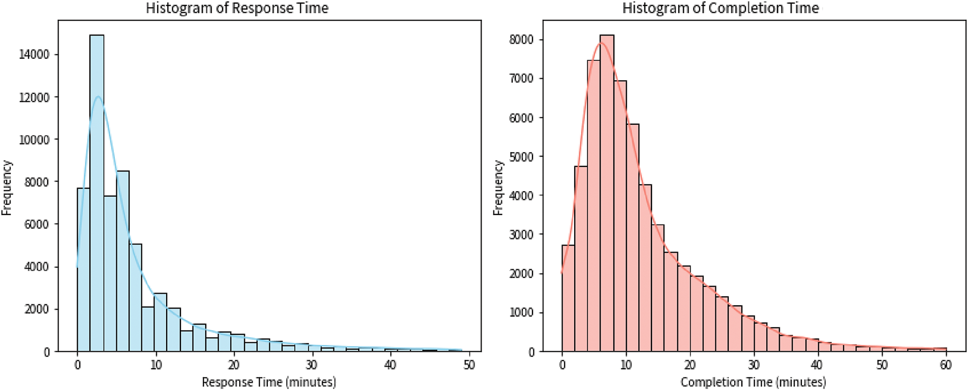
Figure 1: Histogram of task response time and task completion time

We normalized our data using Min-Max normalization, scaling it to [0, 1] to maintain distribution and improve model training. This adjustment ensures proportional alignment of feature values, enhancing performance. In addition, we used the interquartile range (IQR) method to remove task-specific outliers. For the i-th task type, IQRi is determined by Q3i−Q1i, where Q1i and Q3i denote the first and third quartiles, respectively. The lower bound LBi is determined by Q1i−1.5×IQRi, and the upper bound UBi is determined by Q3i+1.5×IQRi. Table 2 provides the corresponding code for each task, while Fig. 2 shows the distribution of each task before and after removing outliers. The top of Fig. 2 shows boxplots of different job types before removing outliers. These plots reveal several outliers, particularly for J03 (oxygen cylinder replacement) and J07 (instrument delivery). The bottom of Fig. 2 displays boxplots after removing these outliers. The distributions become more concentrated, with fewer extreme values. However, even after removing outliers, J03’s completion times ranged from 0.2 to 0.45, exceeding those of other tasks (typically < 0.1). This difference is due to the critical nature of handling oxygen cylinders. Many factors can contribute to extended completion times, including strict safety protocols, logistical challenges involving heavy and large transport, and coordination requirements with medical staff. Additionally, J07 exhibits a wide range of completion times due to varying handling requirements for different medical instruments. Some items may require extra care, and accessibility within the hospital can vary significantly. Special sterilization, preparation procedures, and urgency levels may also impact delivery times. The last step of data preprocessing is label encoding, where features such as category, tool, age, transfer type, and work interval are converted from categorical to numerical data. The results are shown in Table 3.

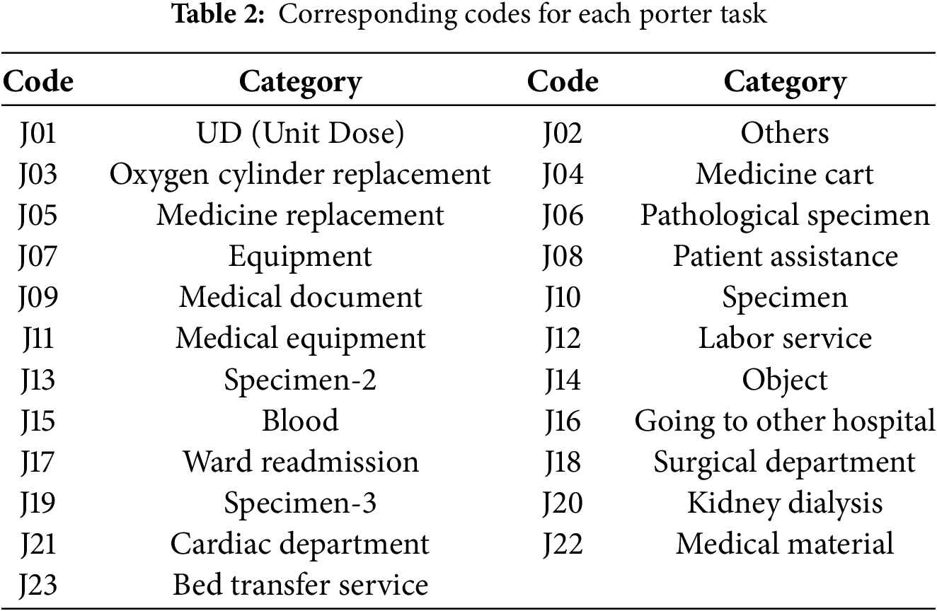
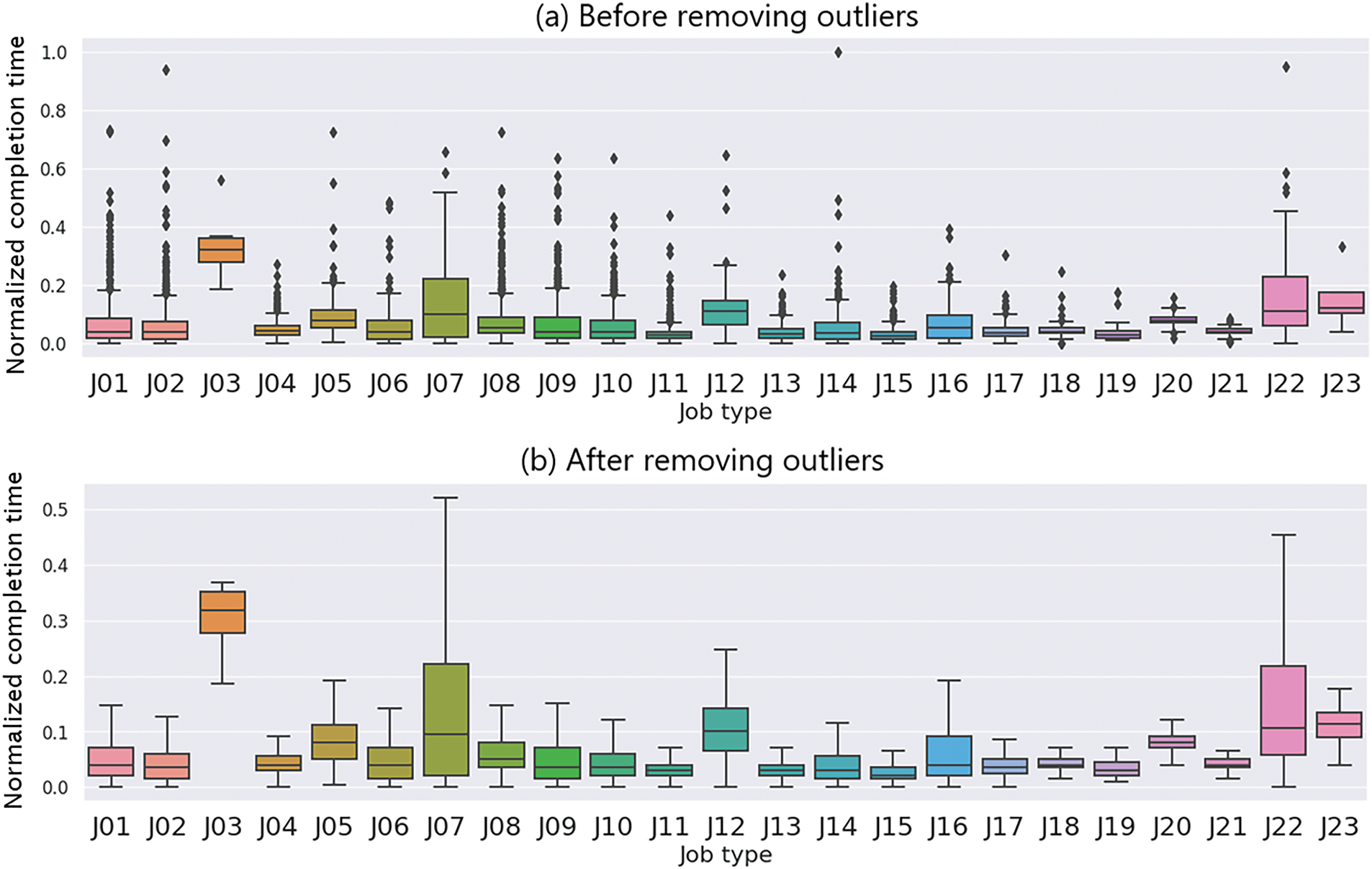
Figure 2: Boxplot of normalized completion time for different job types, shown before (a) and after (b) removing outliers using the IQR method. After outlier removal, most job types show reduced variation. However, J03, J07, and J22 still show relatively wide ranges, likely due to complex handling, coordination requirements, or job-specific variability

3.3 Feature Selection for Porter Tasks

There are three main categories of feature selection methods: Filter, Wrapper, and Embedded methods [24]. Filter methods remove features based on statistical values and a threshold. Wrapper methods add or remove features based on a target function. Embedded methods use machine learning models to further remove features below a threshold based on the fit of the data. In this section, we describe how features are selected by each method, respectively. The selected features are applied for time prediction in Section 4, and the experimental results of the performance comparison are presented in Section 5.

3.3.1 Filter Method

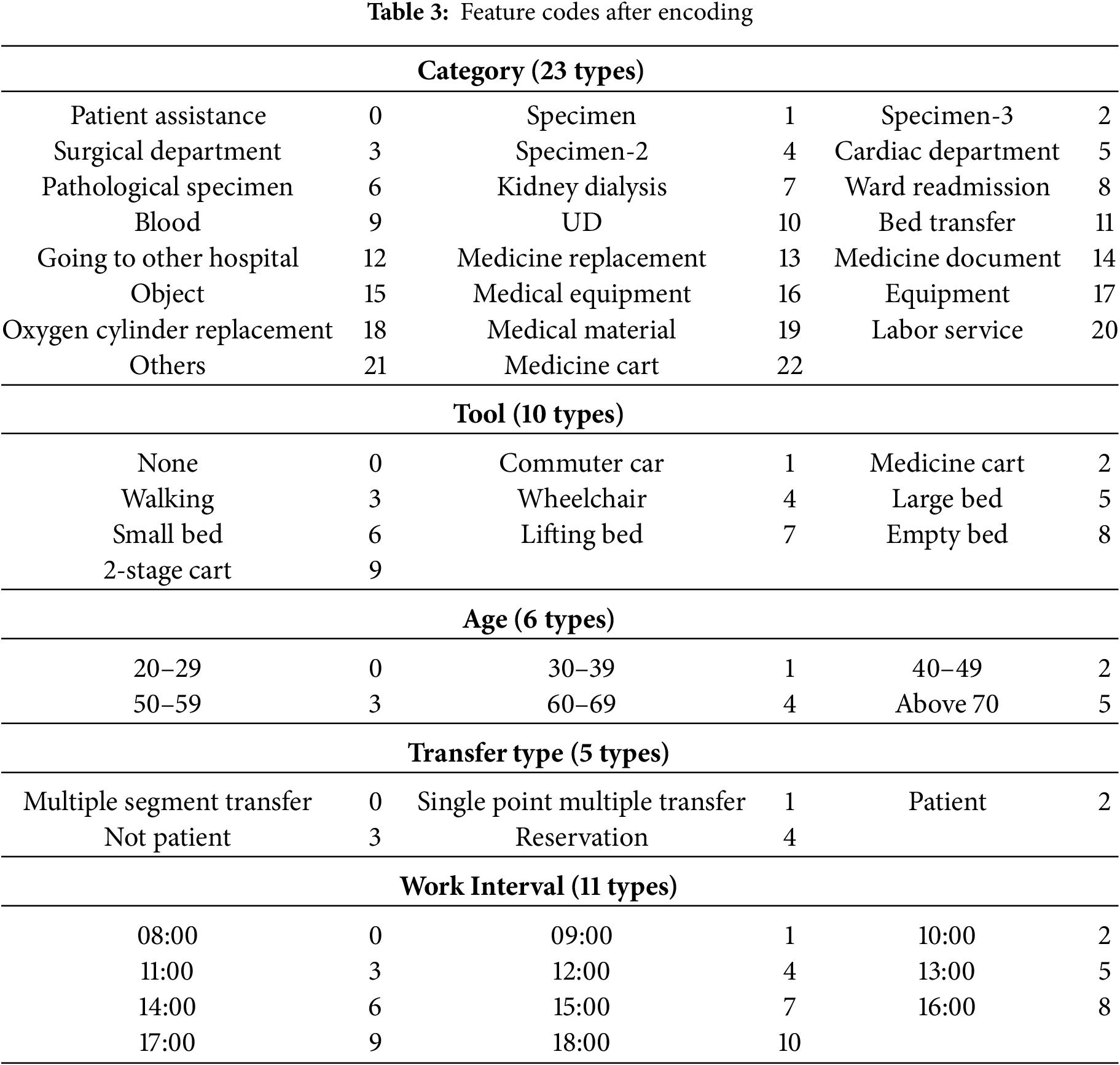
Filter method uses statistical analysis like correlation to pinpoint the most relevant features for prediction. This helps select the most informative features, leading to a more focused and efficient model. Fig. 3 shows a heatmap of feature correlations. It visualizes the Pearson correlation coefficients between eleven features related to task performance, including task response time and completion time. From this analysis, we found that task response time is most positively correlated with Category (coefficient: 0.22). For completion time, the strongest positive correlation is with Tool (coefficient: 0.30), while the strongest negative correlation is with Category. After encoding categorical data numerically, we further observed some interesting patterns. Completion time tends to increase with higher values for Tool and Distance. Specifically, certain tools like 2-Stage Cart and Empty Bed, as well as longer distances, are associated with longer completion times. Based on this correlation analysis, we identified Tool and Distance as important features for our model. These features were retained because their strong positive correlation with task response time and completion time suggests a direct and interpretable contribution to the model’s predictive accuracy.

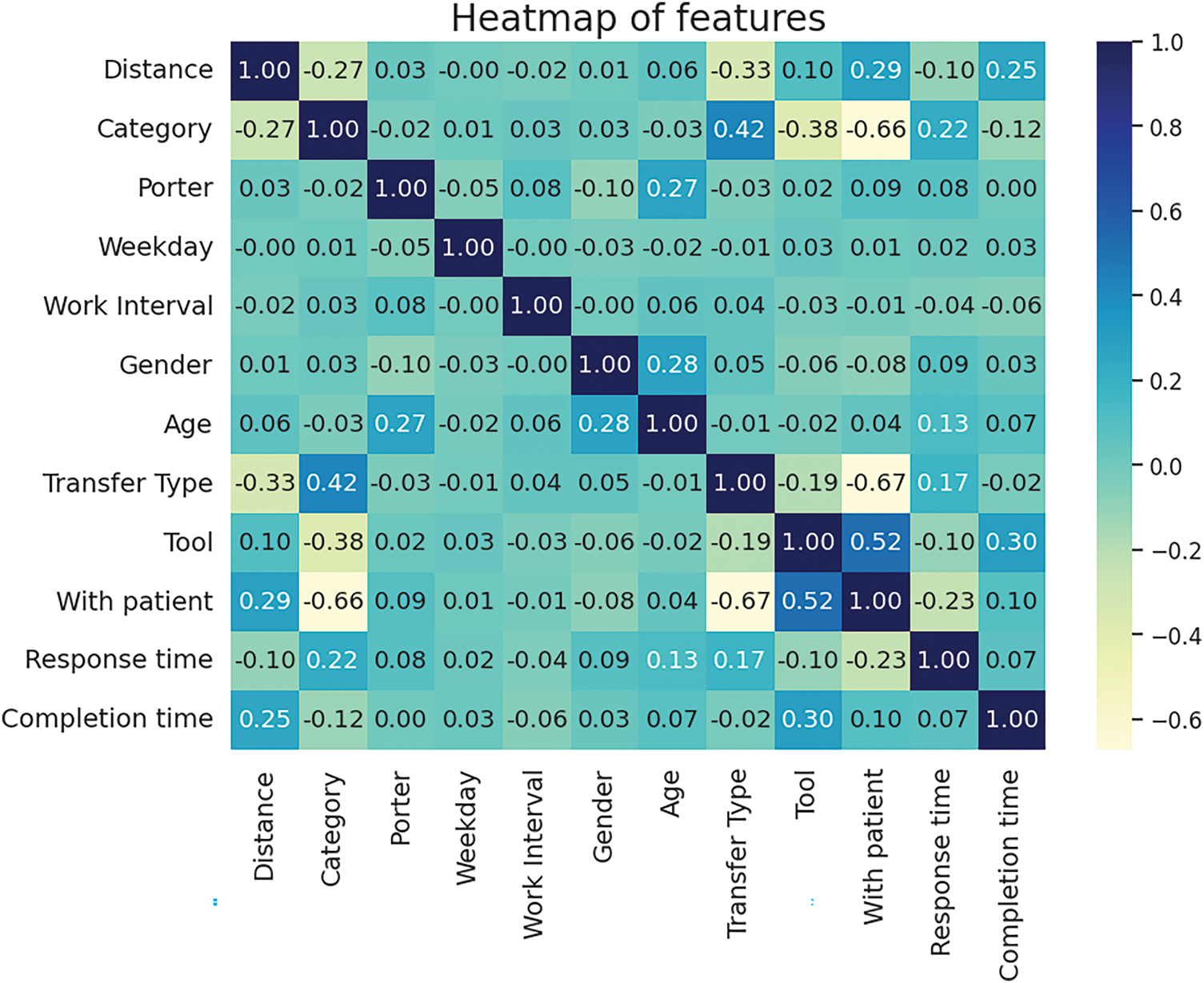
Figure 3: Heatmap of feature correlations

3.3.2 Wrapper Method

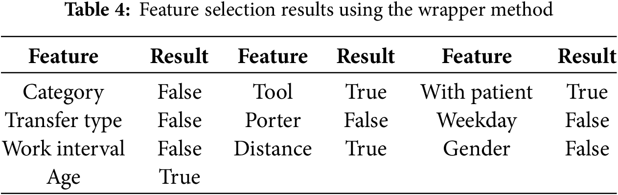
Wrapper method requires more computation time compared to the filter method because it uses a greedy approach to find the optimal feature combination. Although it is more computationally intensive, the wrapper method may achieve better model performance. It can be divided into four different approaches: Step Forward Feature Selection (SFFS), Step Backward Feature Selection (SBFS), Exhaustive Feature Selection (EFS), and Bidirectional Search (BS). SFFS initially starts with an empty feature set and adds one feature at a time, while SBFS starts with all features and removes them one by one. EFS tests all possible feature combinations, while BS uses both SFFS and SBFS simultaneously to obtain the best possible solution. In this study, we employed the SFFS and SBFS methods for feature selection using the wrapper approach, as these methods balance computational efficiency with effective feature selection. The feature selection results of the wrapper method are presented in Table 4. Both SFFS and SBFS selected the same four features: Tool, With Patient, Distance, and Age, because they consistently reduced MAE during iterative evaluation. Other features were excluded as they did not contribute to performance improvement and were likely less relevant to the prediction task.

3.3.3 Lasso Embedded Method

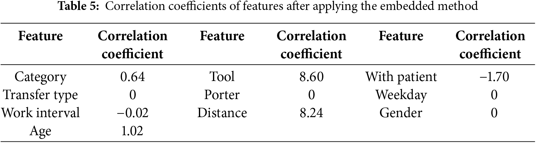
Lasso (L1) embedding is the third method of feature selection. According to Chandrashekar, feature selection can remove irrelevant features from the prediction target, which reduces the number of features, improves model accuracy, shortens runtime, and helps avoid overfitting [25]. In this study, the regularization strength for the Lasso method is determined by adjusting the alpha value, with alpha = 0.1 used as the parameter. Unlike filtering methods, L1 embedding retains only features with non-zero coefficients, without considering their specific impact on the prediction target. Table 5 displays the coefficients for each feature. After removing those with zero coefficients, a total of six features were retained: Category, Tool, With Patient, Work Interval, Distance, and Age. These features were kept because their non-zero coefficients indicate a stronger contribution to the model’s internal objective function, while others were excluded due to having no measurable effect on the prediction outcome under L1 regularization.

4  Methods of Transferring Time Prediction

The average method is the most straightforward approach to predict transfer time. However, in practice, porters’ tasks can be influenced by various factors, such as temporal and spatial context, individual porter characteristics, varying task conditions, and unexpected business needs that may extend delivery time. Relying solely on the average as the prediction value can lead to significant errors and discrepancies from the actual situation. Therefore, in this section, we discuss several machine learning methods for Transferring time prediction. These methods include the decision tree algorithm, random forest algorithm, and gradient boost algorithm. We focused on three tree-based models: decision tree, random forest, and gradient boosting because they are well suited for tabular data, robust to feature interactions, and widely used in healthcare-related tasks. These models strike a balance between predictive performance and interpretability, making them practical for hospital settings where model transparency and low deployment cost are important.

4.1 Decision Tree Algorithm

The Decision Tree (DT) is a commonly used tree-based algorithm that can be applied to both regression and classification problems. The basic classification method involves continuously branching downwards based on split point rules, and as the height of the tree increases, its classification of data becomes more rigorous. The DT generates different trees based on different training data. In this paper, branches are continuously generated downwards in a greedy manner based on the importance of different features in the delivery data until the sample set is completely divided. As this paper deals with a regression problem, Mean Squared Error (MSE) is used as the impurity measure instead of Gini Index or Entropy in classifiers.

According to the research proposed by Breiman, when constructing a DT, the algorithm calculates the Sum of Squared Errors (SSE) for each feature and sample size of the splits, and selects the feature with the smallest SSE as the splitting feature [26]. This process is carried out recursively until the MSE of the leaf node reaches zero. In Eq. (1), F represents the feature set of the dataset, which consists of k features. The sample sizes of the left subtree set and right subtree set for a particular feature are shown in Eqs. (2) and (3), respectively. Sleft∣Fk represents the left subtree of feature Fk with n data, while Sright∣Fk represents the right subtree of feature Fk with m data.

F=F1,F2,…,Fk(1)

Sleft∣Fk=x1,x2,…,xn(2)

Sright∣Fk=x1,x2,…,xm(3)

Eq. (4) represents the algorithm for calculating the SSE of a given feature Fk. In this equation, n∣Sleft denotes the number of data in the left subtree, m∣Sright denotes the number of data in the right subtree, yi represents the i-th true value. ȳleft represents the average of all true values in the left subtree, and ȳright represents the average of all true values in the right subtree. i in the left and right subtrees traverse each data in their sets to calculate. After that, the splitting with the minimum SSE value is selected as the root node of the DT.

SSE∣Fk=min(∑i=0n∣Sleft(yi−y¯left)2+∑i=0m∣Sright(yi−y¯right)2)(4)

After constructing the DT, we can calculate the Feature Importance (FI) for each feature based on the classification criteria. FI is determined by the feature value used for splitting, the number of samples split on the feature, and the MSE resulting from the split. Eq. (5) expresses the calculation of FI for each node, where Wnode represents the number of samples in the node, IMnode denotes the impurity of the node measured by MSE, Wleft and Wright represent the number of samples of the left (right) node, and IMleft and IMright represent the impurity of the left (right), respectively.

FInode=Wnode⋅IMnode−Wleft⋅IMleft−Wright⋅IMright(5)

Feature importance is calculated by summing the importance values of all nodes that split on a given feature. The importance value for each feature is then divided by the total importance of all features in the tree, as shown in Eq. (6). Here, FIi is the importance of the i-th feature, wi is the sum of its importance, and ∑j=1k|wj| is the total importance of all features.

FIi=|wi|∑j=1k|wj|(6)

4.2 Random Forest Algorithm

The Random Forest (RF) algorithm is a tree-based model that builds on the Decision Tree (DT) concept [27]. It consists of multiple decision trees and is an ensemble learning method that combines several models to create a stronger and more robust model. Individual decision trees can suffer from overfitting, especially when they are too deep, leading to poor performance. RF mitigates this issue by using multiple decision trees with varying depths, reducing the risk of overfitting and improving overall performance. Unlike classification trees that use a voting mechanism to predict the class, RF in regression problems averages the predictions from all the trees in the forest to make its final prediction.

4.3 Gradient Boost Algorithm

The Gradient Boosting algorithm is an extension of Random Forest (RF) [26]. In Gradient Boosting, each tree built during the training process refers to the previous trees, computing the errors in their predictions. These errors are then used to adjust the subsequent tree’s predictions according to the learning rate. Unlike in RF, where each tree is independent and doesn’t affect the other trees’ predictions, in Gradient Boosting, each tree is related to the preceding ones. This interdependence between the trees is one of the main differences between Gradient Boosting and RF. To optimize the hyperparameters of the Gradient Boosting model, Grid Search is used to fine-tune the model and slightly improve the regression prediction results.

5  Experiment Results

5.1 Evaluation Metrics and Setup

To perform our analysis, we split the data into an 80% training set and a 20% testing set, comprising 66,444 and 16,611 samples, respectively. In this study, since we are dealing with a regression problem, we utilize Mean Squared Error (MSE) and Mean Absolute Error (MAE) as evaluation metrics, as shown in Eqs. (7) and (8), respectively.

MSE=1n∑i=1n(truei−predi)2(7)

MAE=1n∑i=1n|truei−predi|(8)

These equations indicate that in a dataset of size n, truei represents the true value of the i-th data point, and predi represents the predicted value of the i-th data point. A smaller value for both metrics indicates better model performance. The main difference between the two metrics is that MSE is more sensitive to outliers in the predicted values, as the squaring operation gives these values more weight. In contrast, MAE is less sensitive to outliers, as it uses the absolute value instead. In practical applications, MAE may be preferred as it provides a more intuitive evaluation of the model’s performance. In this paper, MSE is reported in units of (min2), and MAE is reported in units of (min).

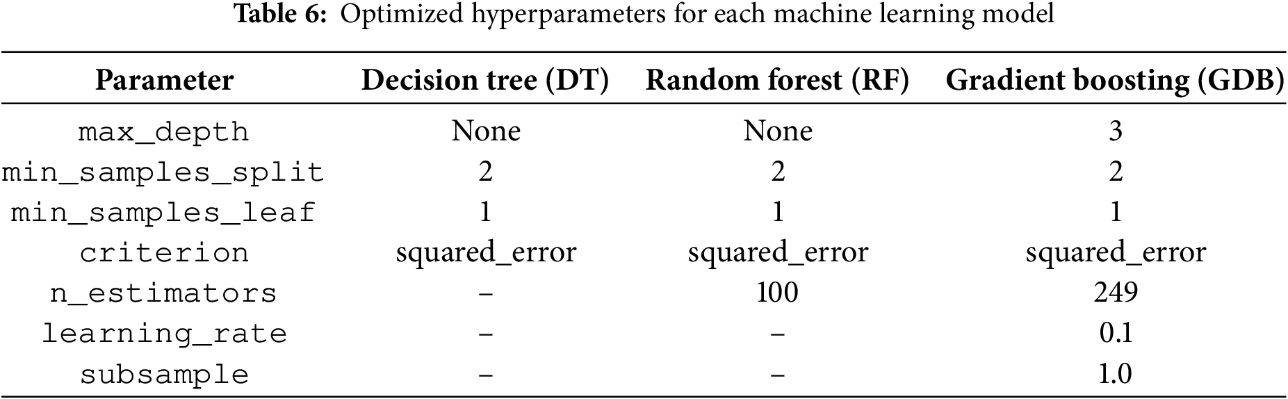
The experimental environment used in this work consists of an Intel(R) Xeon(R) CPU @ 2.20 GHz with 12 GB RAM, running on Google Colab [28]. In addition to MSE and MAE, we also compare the execution time of each algorithm in the following experiment. We used the following hyperparameters for the individual models. For the DT model, we set max_depth to None (no maximum depth limit), min_samples_split to 2, min_samples_leaf to 1, and used the default regression criterion “squared_error”. For the RF model, we used n_estimators = 100, max_depth = None, min_samples_split = 2, min_samples_leaf = 1, and “squared_error” as the criterion. These settings follow common defaults in standard implementations. We did not perform hyperparameter tuning for individual models to avoid possible overfitting. Instead, we conducted a grid search to optimize the weighting of each model in the ensemble model (Section 5.4). Table 6 summarizes the optimized hyperparameters used for training the decision tree, random forest, and gradient boosting models. To strengthen the robustness of the results, we conducted 5-fold cross-validation. The results show that the model’s mean absolute error (MAE) remains consistent across the folds, supporting the model’s generalization capability and robustness.

5.2 Accuracy of Task Response Time Prediction

5.2.1 Statistical Mean for Prediction

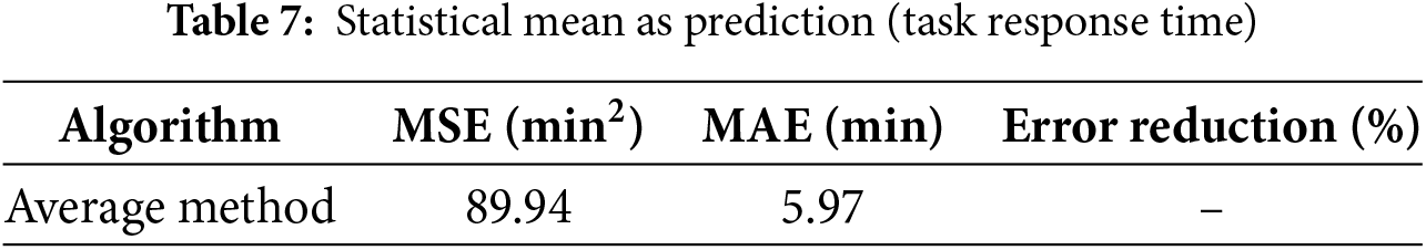
The task response time is determined by subtracting the dispatch time from the arrival time. The arrival time is the time the porter arrives at the request unit. To evaluate the performance of our models, we aim for lower values of MSE and MAE, as they indicate better model accuracy and predictive capability. The average algorithm uses historical data to predict task response time. Table 7 presents the error for predicting task response time. The MSE and MAE values are 89.94 and 5.97, respectively. The average method serves as the baseline for comparison.

5.2.2 Effect of Feature Selection on Accuracy

Table 8 shows a comparison of algorithms with different feature selection methods. It is observed that the DT model has the poorest performance, with an MAE of 4.2, while the RF and GDB models perform better, with MAE values of 3.13 and 3.04, respectively. The improvement in performance of the RF and GDB models over the DT model is 25.47% and 27.61%, respectively. Moreover, in terms of predicting task response time, the GDB model exhibits the best performance among the three tree-based models. It is also observed that for both the RF and GDB models, after filter feature selection, the models are reduced to DT, and their performance does not improve. Among the various feature selection methods used in the prediction models, the only model that showed significant improvement in performance was the DT model with the filter feature selection method. Although the DT model with the filter method is not better than the GDB model with all features, it has an advantage in computation time, requiring only 2 features to operate and being up to 186 times faster than the best GDB model. In addition, for both DT and RF models, the performance after feature selection is noticeably lower compared to the models trained with all features. This suggests that specific models require appropriate feature selection methods to achieve optimal performance.

Table 9 presents the best performance comparison of each algorithm in predicting task response time. The average method, with a mean absolute error (MAE) of 5.97 min, serves as the baseline for comparison. Using machine learning with decision trees (DT) reduces the MAE to 3.48 min, a 41.7% improvement over the average method. Additionally, gradient boosting (GDB) achieves the best performance with an MAE of 3.04 min, reducing the error by 49% compared to the average method.

Fig. 4 presents the boxplot of errors for different job types based on the best-performing model, GDB. The boxplot indicates that the task types “Medicine Replacement” and “Going to Other Hospital” have a relatively high dispersion of errors, suggesting that these two types of tasks are more susceptible to additional factors that may affect their task response time compared to other job types.

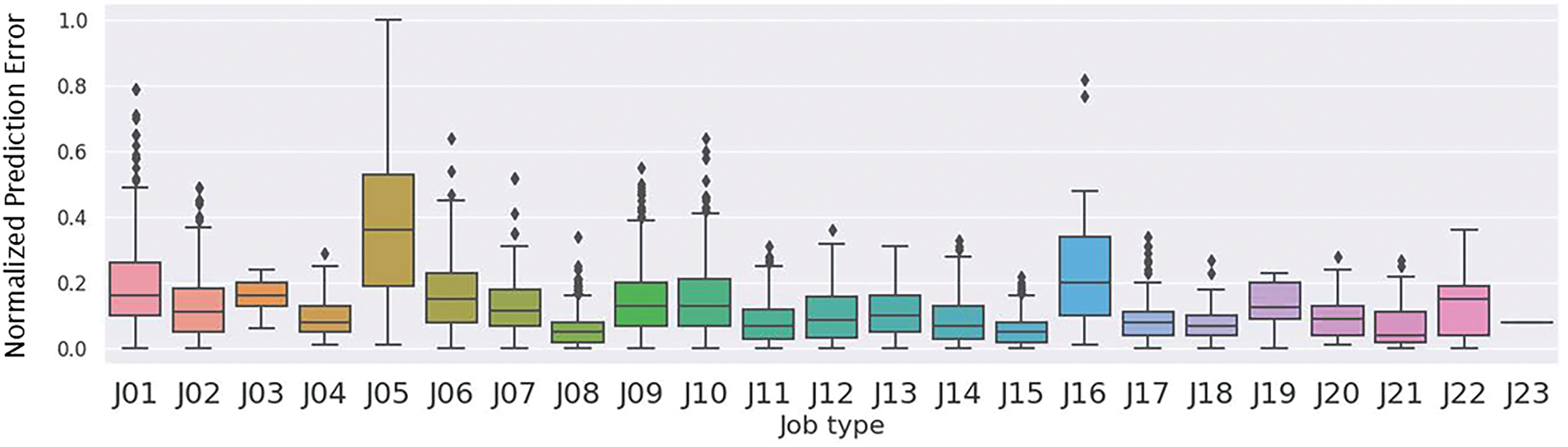
Figure 4: Normalized prediction error of task response time by job type using the GDB model. J05 (Medicine Replacement) and J16 (Going to Other Hospital) show higher variability in error, suggesting they are more likely influenced by task-specific uncertainties

5.3 Accuracy of Task Completion Time Prediction

5.3.1 Statistical Mean for Prediction

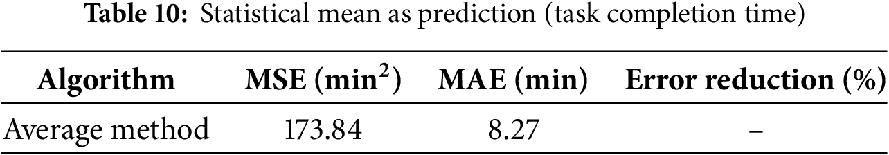
The task completion time is determined by subtracting the arrival time from the completion Time. Table 10 presents the prediction errors using the average time of each task type as the predicted completion time. The MSE is as high as 173.84, and the MAE is also high at 8.27. This is expected, as the prediction error may be affected by various factors such as different temporal and spatial backgrounds during each task, different porters, different task conditions, or unforeseen circumstances that cause delays in completion time. Therefore, if the average time is used as the sole predictor, the results may deviate significantly from the actual situation. The average method serves as the baseline for comparison.

5.3.2 Effect of Feature Selection on Accuracy

Table 11 presents a performance comparison of each algorithm with different feature selection methods for task completion time prediction. The results indicate that the DT model performed the worst, with an MAE of 5.84. In contrast, the RF model showed significant improvement over the DT model, achieving an MAE of 4.58, which represents a 21.57% enhancement. Among the three models, the Gradient Boosting (GDB) model achieved the best performance for porter task completion time prediction, with the lowest MAE of 4.51 min when using all features. Further analysis shows that feature selection impacts the models differently. The DT model’s performance improved significantly after feature selection, with a 34.46% reduction in MSE and a 13.87% reduction in MAE. This suggests that the DT model can benefit from appropriate feature selection. However, the RF and GDB models exhibited deteriorated performance after feature selection using the correlation coefficient filter method compared to using all features. This underscores the importance of quality feature engineering, implying that feature selection should be customized based on each model’s characteristics to achieve optimal results.

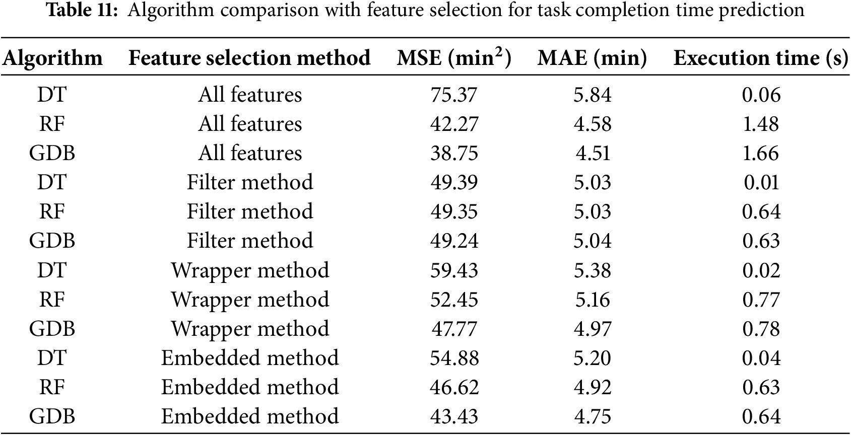
When comparing feature selection methods, the models generally performed worse with the wrapper method than with the filter method. However, the Decision Tree (DT) model still showed improvement, reducing its Mean Absolute Error (MAE) from 5.84 to 5.38, a 7.8% enhancement. Although all three models performed worse with the embedded method compared to the filter method, they still outperformed the wrapper method. Notably, the embedded method, which added only one additional feature, led to the DT model achieving the best performance, with an MAE reduction from 5.84 to 5.20, representing a 10.9% improvement compared to using all features. Furthermore, similar to the results for task response time, the computation time of the DT model after applying the filter method was up to 166 times faster than the best-performing Gradient Boosting Decision (GDB) model. As data size increases, computation time becomes a critical factor for achieving real-time performance.

Table 12 shows the best performance results obtained by training three tree-based models and predicting the required time for each task based on their respective mean values. As shown in the table, the MSE and MAE values obtained using the mean value as the prediction are significantly higher than those obtained using the three tree-based models. In practical terms, relying solely on statistical data for time estimation is not robust. The DT model achieved the best performance with a MAE of 5.03, representing a 39.17% decrease in the error rate compared to the base case. This result is promising for hospital time resource management. The RF model, which shares a tree-based structure with DT, achieved a slightly better result with a MAE of 4.58, representing a 44.61% decrease in the error rate. The GDB model achieved the best performance among the three models with a MAE of 4.51, representing a slight improvement over RF and a 45.46% decrease in the error rate compared to the base case. Fig. 5 displays the error boxplots for different task types based on the best algorithm, GDB. Tasks such as “Oxygen Cylinder Replacement” and “Equipment” exhibit larger error ranges. This reinforces the notion that when data is more dispersed, the predictions tend to be less accurate.

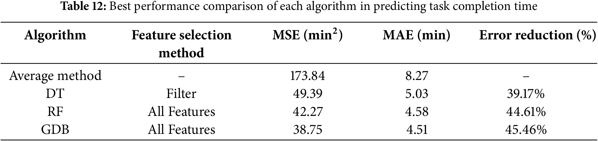
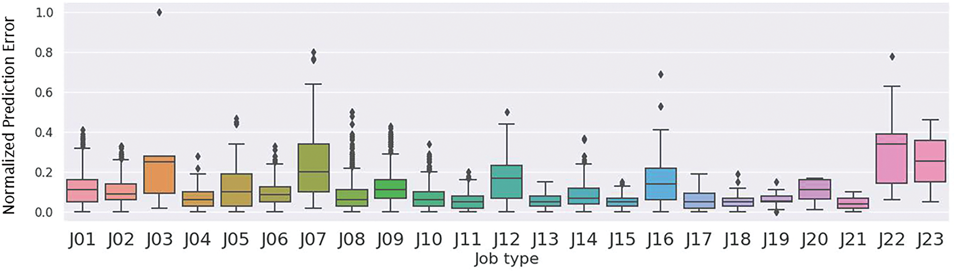
Figure 5: Normalized prediction error of task completion time by job type using the GDB model. J03 (Oxygen Cylinder Replacement), J07 (Equipment), and J22 (Medical Material) exhibit higher prediction errors compared to other task types, suggesting that task complexity, variability in handling, or coordination requirements may contribute to reduced model accuracy

5.4 Accuracy of Ensemble Modeling

An ensemble model is a machine learning technique that combines multiple individual models to make predictions or decisions. It can improve overall performance and generalization ability compared to using a single model, leading to better predictions or decisions [29]. In this study, we proposed an integrated model that represents the ensemble of the three best-performing tree-based algorithms: DT, RF, and GDB. To ensure that the ensemble combines the strongest predictors from each base model, we adopt the best-performing configuration based on earlier experimental results. Specifically, for predicting task response time, we combine DT with features selected by the filter method including Tool and Distance, RF with all features, and GDB with all features. The same configuration is used for predicting task completion time, ensuring that the ensemble leverages the optimal predictive performance of each individual model. The integrated model utilizes optimal weight allocation for each model to achieve the best prediction results, as shown in Eq. (9), where βi represents the weight for the i-th model, and the sum is equal to 1. We used grid search to find the optimal weight combinations for the three models that minimized the prediction errors [12]. This involves creating a grid of all possible combinations of hyperparameters and evaluating each combination using a performance metric.

∑i=13βi=1.(9)

As Table 13 shows, the best weights for task response time were [0.02, 0.16, 0.82], resulting in an MSE of 17.19 and an MAE of 3.00. On the other hand, for task completion time, the best weights were [0.03, 0.28, 0.69], resulting in an MSE of 36.89 and an MAE of 4.42. By utilizing grid search to find the optimal weights for each model, we can further build another prediction model with the best performance. The results indicate that the integrated model slightly outperforms each individual model and achieves the best prediction accuracy. In summary, since the mean task response time is 7.17 min and the mean completion time is 12.11 min, the ensemble model’s 3.00-min error for response time prediction is approximately 42% of the mean, and the 4.42-min error for completion time prediction is approximately 36% of the mean. These levels of accuracy, around 3 to 4 min, are sufficient for practical applications such as delay detection and resource allocation.

5.5 Feature Importance Analysis

Based on our analysis, the feature importance values obtained from the decision tree model are shown in Fig. 6. According to this figure, the decision tree (DT) was primarily constructed using the features Distance, Tool, and Work Interval, with corresponding importance values of 0.227, 0.162, and 0.144, respectively. The tree makes decisions based on the relative weights of these features: Distance is considered first, followed by Tool at the second level, and Work Interval at the third. As the tree extends deeper, the decision rules become more complex, leading to more accurate regression calculations. Fig. 7 shows the feature importance in the RF model. This importance is calculated by averaging the weights of each feature across all trees. The top three features are Distance, Tool, and Work Interval, with importance scores of 0.221, 0.174, and 0.133, respectively. In comparison to a DT, the RF model places more emphasis on Distance and Tool, while Work Interval has a smaller influence.

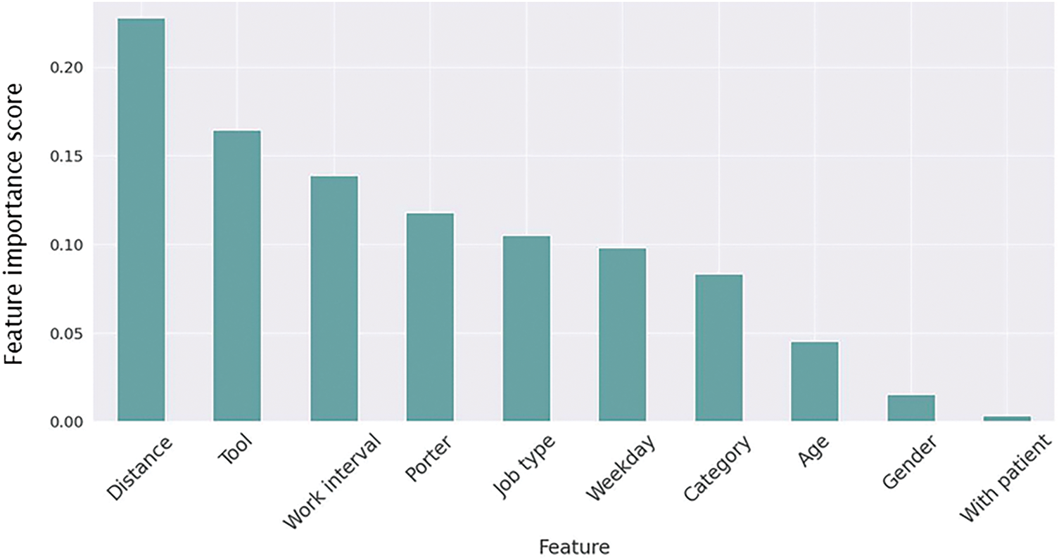
Figure 6: Feature importance from the decision tree model. Distance, tool, and work interval were most influential, while gender and with-patient had limited impact

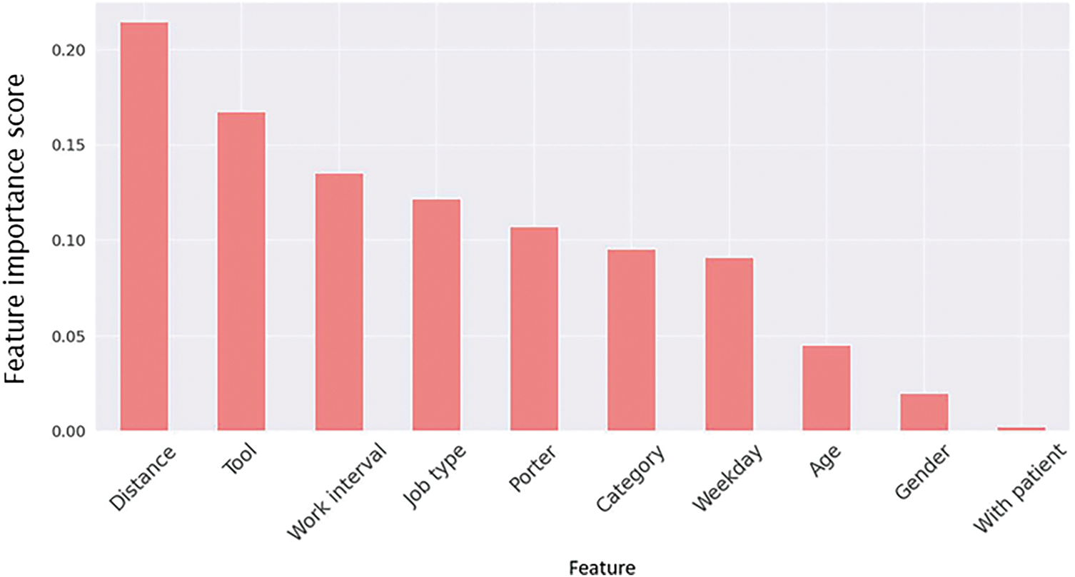
Figure 7: Feature importance from the random forest model. Distance and tool ranked highest, while work interval had slightly less influence than in the decision tree

In Fig. 8, it can be observed that in the Gradient Boosting model, the top three features in terms of importance are Tool, Distance, and Category, with scores of 0.299, 0.256, and 0.203, respectively. Compared to the Decision Tree (DT) and Random Forest (RF) models, Tool is more important than Distance in the Gradient Boosting model. Furthermore, for hyperparameter tuning in the Gradient Boosting model, the grid search method was utilized. This approach allows a range of parameter combinations to be tested, and the best combination is then selected, leading to the training of the optimal model.

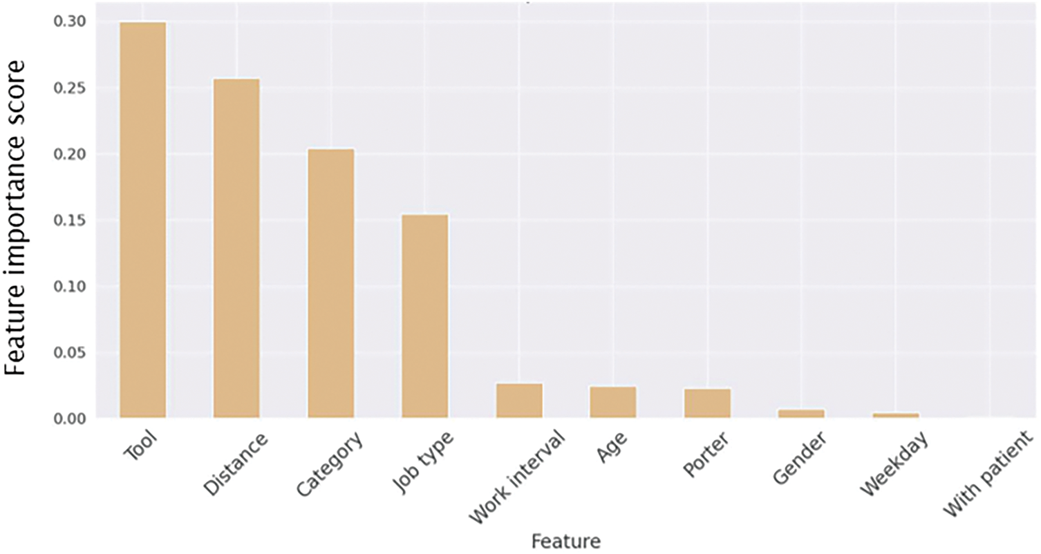
Figure 8: Feature importance from the gradient boosting model. Tool, Distance, and Category were the most important features, with Tool surpassing Distance, unlike in the DT and RF models. Hyperparameter tuning via grid search optimized the model

Based on our analysis, the most important features were distance, tool type, and work interval. Distance consistently ranked as the top feature across the decision tree, random forest, and gradient boosting models. This aligns with real-world operations, as porter tasks naturally take longer when the distance between pickup and delivery points increases, reflecting the physical layout and size of the hospital. Tool type was also a key factor, as tasks involving specialized equipment (e.g., large beds or wheelchairs) typically require more preparation, leading to longer completion times. Work interval was another influential feature, as hospital workload and staffing levels vary across different shifts (for example, busy morning rounds vs. quieter night hours), affecting porter availability and travel speed.

5.6 Usage Scenarios and Discussion

This paper presents a time prediction model that can be applied to hospital porter task time prediction. The application of this model can be categorized into three types depending on the user. Firstly, on the ward side, when a request is made, the dashboard can display the predicted arrival time in real-time. With the assistance of time prediction, healthcare professionals can make appropriate time arrangements within the predicted time and reduce time waste, thereby further improving the overall work efficiency of the hospital. Secondly, on the dispatch center side, which controls the entire dispatch process, the time prediction feature can more effectively manage task execution times. Unlike in the past, where the dispatch center could only wait for porter reports, the center can now track progress in advance if a task is delayed, thereby avoiding wasted time. Thirdly, for patients and their accompanying family members assigned to a sickbed, the exact arrival time of the porter can be known in real-time, allowing them to effectively arrange their time.

Furthermore, integrating this prediction system with the existing porter dispatch system through an API offers additional benefits. With data collected in a standardized format for training, the API can be designed to handle data input and output, allowing users to upload data and obtain prediction results seamlessly. Additionally, deploying the server in the cloud enables real-time operation, facilitating the prediction of task response time, task completion time, and providing processed porter delivery data for management personnel to utilize effectively. This integration not only streamlines the prediction process but also empowers management personnel with valuable insights and actionable information.

While the dataset is large and diverse within a single hospital (covering 75 porters and over 58,000 tasks), it is limited to one hospital in Taiwan. As a result, differences in hospital layout, porter training, task protocols, and staffing models across institutions could affect the generalization of the model. Adapting the model to new environments may also require retraining or fine-tuning. Therefore, future work should validate the model on external datasets from other institutions to ensure broader applicability.

Moreover, while age and gender were included as features due to their potential relevance to task duration, we are aware that their use may raise ethical concerns, such as the risk of making unfair predictions based on a person’s age or gender. Although this study did not focus on fairness issues, we acknowledge the importance of using demographic information responsibly and will explore fairness-aware modeling in future work to ensure equitable outcomes. In addition, while tree-based models offer a good balance between performance and interpretability, they may not capture uncertainty or complex nonlinear relationships. A recent study [30] applied a Bayesian neural network to predict crash severity and showed improved performance over traditional models. Exploring such probabilistic models may be considered in future work to further enhance prediction accuracy and uncertainty estimation.

6  Conclusion

This paper proposes a machine learning-based algorithm for time prediction and designs a data preprocessing and feature selection approach to identify the optimal feature selection method for each algorithm. The results show that using the wrong feature selection method can significantly impact predictive ability, with RF and GDB degrading to the performance level of DT, thereby losing their optimal predictive ability. In addition to existing tree algorithms, we also propose an integrated model, EM, and use grid search to find the optimal parameters. The results demonstrate that our proposed EM has the best predictive ability, with MAEs of 3 min for task response time and 4.42 min for task completion time. The prediction accuracy for both task response time and task completion time improved by 52.1% and 46.55%, respectively, compared to an algorithm using the average of historical data. The time prediction system enables all three types of users to more effectively manage their time, reducing unnecessary wait times for patients, allowing ward staff to schedule work based on estimated arrival times and avoid delays for transport personnel, and optimizing scheduling for the transport center. This algorithm can also be applied to predicting waiting times in outpatient or emergency departments, thereby enhancing the efficiency of time management in healthcare through technological means. Future research will focus on predicting time related to hospital business efficiency, with the aim of improving time management in healthcare despite limited medical capacity. In addition to predicting transport task time, we will also investigate time prediction in specific hospital departments, such as emergency rooms. By identifying features that affect patient flow through scientific data analysis, we aim to provide hospitals with effective management and decision-making tools. To further enhance the applicability of our approach, future work will include validating the model using multi-center datasets to improve generalizability. We also plan to explore other types of machine learning models, such as regression or neural networks, to verify the robustness and adaptability of our method across different modeling paradigms. In addition, we will explore hyperparameter tuning of individual models to improve their standalone performance and ensure fairer comparisons within ensemble modeling.

Acknowledgement: We thank Shaowei Wen, Chingmei Tsai, Tzuling Wang and Jiawei Fong for their help in explaining the definition of porter data and the flow of porter services. We would like to thank Jingshan Su for assistance with proofreading.

Funding Statement: This work was supported by National Taiwan University Hospital Yunlin Branch Project NTUHYL 110.C018 and National Science and Technology Council, Taiwan.

Author Contributions: The authors confirm contribution to the paper as follows: Conceptualization, Edward T.-H. Chu, Jiun Hsu, Huimei Wu and Chia-Rong Lee; methodology, Youjyun Yeh, Edward T.-H. Chu; software, Youjyun Yeh; validation, Youjyun Yeh and Edward T.-H. Chu; formal analysis, Youjyun Yeh and Edward T.-H. Chu; investigation, Youjyun Yeh and Edward T.-H. Chu; resources, Edward T.-H. Chu, Jiun Hsu and Huimei Wu; data curation, Youjyun Yeh; writing—original draft preparation, Youjyun Yeh; writing—review and editing, Edward T.-H. Chu; visualization, Youjyun Yeh; supervision, Edward T.-H. Chu and Chia-Rong Lee; project administration, Edward T.-H. Chu and Jiun Hsu; funding acquisition, Edward T.-H. Chu and Jiun Hsu. All authors reviewed the results and approved the final version of the manuscript.

Availability of Data and Materials: Not applicable.

Ethics Approval: Not applicable.

Conflicts of Interest: The authors declare no conflicts of interest to report regarding the present study.

References

1. Lee CR, Chu ETH, Shen HC, Hsu J, Wu HM. An indoor location-based hospital porter management system and trace analysis. Health Inform J. 2023;29(2):14604582231183399. doi:10.1177/14604582231183399. [Google Scholar] [PubMed] [CrossRef]

2. Kurt N, Bakır R, Seyyedabbasi A. Transportation models in health systems. In: Allahviranloo T, Hosseinzadeh Lotfi F, Moghaddas Z, Vaez-Ghasemi M, editors. Decision making in healthcare systems. studies in systems, decision and control. Cham, Switzerland: Springer International Publishing; 2024. p. 429–42. doi:10.1007/978-3-031-46735-6. [Google Scholar] [CrossRef]

3. Ton VM, da Silva NCO, Ruiz A, Pécora JEJr, Scarpin CT, Bélenger V. Real-time management of intra-hospital patient transport requests. Health Care Manag Sci. 2024;27(2):208–22. doi:10.1007/s10729-024-09667-6. [Google Scholar] [PubMed] [CrossRef]

4. Chen J, Li K, Tang Z, Bilal K, Li K. A parallel patient treatment time prediction algorithm and its applications in hospital queuing-recommendation in a big data environment. IEEE Access. 2016;4:1767–83. doi:10.1109/access.2016.2558199. [Google Scholar] [CrossRef]

5. Robbani R, Ullah MW. COV-HM: prediction of COVID-19 patient’s hospitalization period for hospital management using SMOTE and machine learning techniques. In: Proceedings of the 2nd International Conference on Computing Advancements, ICCA ’22; 2022 Mar 10–12; Dhaka, Bangladesh. p. 25–33. [Google Scholar]

6. Alqatawna A, Abu-Salih B, Obeid N, Almiani M. Incorporating time-series forecasting techniques to predict logistics companies’ staffing needs and order volume. Computation. 2023;11(7):141. doi:10.3390/computation11070141. [Google Scholar] [CrossRef]

7. Chien SH, Sencer B, Ward R. Accurate prediction of machining cycle times and feedrates with deep neural networks using BiLSTM. J Manufactu Syst. 2023;68(7):680–6. doi:10.1016/j.jmsy.2023.05.020. [Google Scholar] [CrossRef]

8. Yi J, Yan H, Wang H, Yuan J, Li Y. Learning to estimate package delivery time in mixed imbalanced delivery and pickup logistics services. In: Proceedings of the 32nd ACM International Conference on Advances in Geographic Information Systems, SIGSPATIAL ’24; 2024 Oct 29–Nov 1; Atlanta, GA, USA. p. 432–43. doi:10.1145/3678717.3691266. [Google Scholar] [CrossRef]

9. Zhu T, Luo L, Zhang X, Shi Y, Shen W. Time-series approaches for forecasting the number of hospital daily discharged inpatients. IEEE J Biomed Health Inform. 2017;21(2):515–26. doi:10.1109/jbhi.2015.2511820. [Google Scholar] [PubMed] [CrossRef]

10. Wang L, Yin Z, Puppala M, Ezeana CF, Wong KK, He T, et al. A time-series feature-based recursive classification model to optimize treatment strategies for improving outcomes and resource allocations of COVID-19 patients. IEEE J Biomed Health Inform. 2022;26(7):3323–9. doi:10.1109/jbhi.2021.3139773. [Google Scholar] [PubMed] [CrossRef]

11. Luo L, Feng Y. Using time series analysis to forecast emergency patient arrivals in CT department. In: 2015 12th International Conference on Service Systems and Service Management (ICSSSM); 2015 Jun 22–24; Guangzhou, China. [Google Scholar]

12. Benevento E, Aloini D, Squicciarini N. Towards a real-time prediction of waiting times in emergency departments: a comparative analysis of machine learning techniques. Int J Forecast. 2023;39(1):192–208. doi:10.1016/j.ijforecast.2021.10.006. [Google Scholar] [CrossRef]

13. Ang E, Kwasnick S, Bayati M, Plambeck EL, Aratow M. Accurate emergency department wait time prediction. Manufact Serv Operat Manag. 2016;18(1):141–56. [Google Scholar]

14. Javadifard H, Sevinç S, Yıldırım O, Orbatu D, Yaşar E, Sişman AR. Predicting patient waiting time in phlebotomy units using a deep learning method. In: 2019 Innovations in Intelligent Systems and Applications Conference (ASYU). Izmir, Turkey; 2019. p. 1–4. [Google Scholar]

15. Wang H, Sambamoorthi N, Sandlin D, Sambamoorthi U. Interpretable machine learning models for prolonged Emergency Department wait time prediction. BMC Health Serv Res. 2025;25(1):403. doi:10.1186/s12913-025-12535-w. [Google Scholar] [PubMed] [CrossRef]

16. Barnes S, Hamrock E, Toerper M, Siddiqui S, Levin S. Real-time prediction of inpatient length of stay for discharge prioritization. J Am Med Inform Assoc. 2015 08;23(e1):e2–10. doi:10.1093/jamia/ocv106. [Google Scholar] [PubMed] [CrossRef]

17. Gutierrez JMP, Sicilia M-A, Sanchez-Alonso S, Garcia-Barriocanal E. Predicting length of stay across hospital departments. IEEE Access. 2021;9:44671–80. doi:10.1109/access.2021.3066562. [Google Scholar] [CrossRef]

18. Triana AJ, Vyas R, Shah AS, Tiwari V. Predicting length of stay of coronary artery bypass grafting patients using machine learning. J Surg Res. 2021;264(10):68–75. doi:10.1016/j.jss.2021.02.003. [Google Scholar] [PubMed] [CrossRef]

19. Golmohammadi D. Predicting hospital admissions to reduce emergency department boarding. Int J Product Econ. 2016;182(1):535–44. doi:10.1016/j.ijpe.2016.09.020. [Google Scholar] [CrossRef]

20. Chen J, Wen Y, Pokojovy M, Tseng TLB, McCaffrey P, Vo A, et al. Multi-modal learning for inpatient length of stay prediction. Comput Biol Med. 2024;171(2):108121. doi:10.1016/j.compbiomed.2024.108121. [Google Scholar] [PubMed] [CrossRef]

21. Silva N, Albertini MK, Backes AR, das Graças Pena G. Machine learning for hospital readmission prediction in pediatric population. Comput Methods Programs Biomed. 2024;244:107980. doi:10.1016/j.cmpb.2023.107980. [Google Scholar] [PubMed] [CrossRef]

22. Nevanlinna J, Eidstø A, Ylä-Mattila J, Koivistoinen T, Oksala N, Kanniainen J, et al. Forecasting mortality associated emergency department crowding with LightGBM and time series data. J Med Syst. 2025 Jan;49(1):9. doi:10.1007/s10916-024-02137-0. [Google Scholar] [PubMed] [CrossRef]

23. Cheng N, Kuo A. Using long short-term memory (LSTM) neural networks to predict emergency department wait time. Stud Health Technol Inform. 2020 Jun;272:199–202. doi:10.3233/SHTI200528. [Google Scholar] [PubMed] [CrossRef]

24. Jović A, Brkić K, Bogunović N. A review of feature selection methods with applications. In: 2015 38th International Convention on Information and Communication Technology, Electronics and Microelectronics; 2015 May 25–29; Opatija, Croatia. p. 1200–5. doi:10.1109/mipro.2015.7160458. [Google Scholar] [CrossRef]

25. Chandrashekar G, Sahin F. A survey on feature selection methods. Comput Elect Eng. 2014;40(1):16–28. doi:10.1016/j.compeleceng.2013.11.024. [Google Scholar] [CrossRef]

26. Breiman L, Friedman J, Olshen RA, Stone CJ. Classification and regression trees. Boca Raton, FL, USA: Routledge; 2017. 358 p. [Google Scholar]

27. Breiman L. Random forests. Mach Learn. 2001;45:5–32. [Google Scholar]

28. Bisong E. Building machine learning and deep learning models on Google Cloud Platform: a comprehensive guide for beginners.Ottawa, ON, Canada: Apress; 2019. doi:10.1007/978-1-4842-4470-8. [Google Scholar] [CrossRef]

29. Sagi O, Rokach L. Ensemble learning: a survey. Wiley Interdiscip Rev Data Min Knowl Disc. 2018;8(4):e1249. doi:10.1002/widm.1249. [Google Scholar] [CrossRef]

30. Arifeen SU, Ali M, Macioszek E. Analysis of vehicle pedestrian crash severity using advanced machine learning techniques. Arch Transp. 2023;68(4):91–116. doi:10.61089/aot2023.ttb8p367. [Google Scholar] [CrossRef]