
 Submit a Paper
 Propose a Special lssue
 Open Access
ARTICLE

Magneto-Electro-Elastic 3D Coupling in Free Vibrations of Layered Plates
Department of Mechanical and Aerospace Engineering, Politecnico di Torino, Torino, 10129, Italy
* Corresponding Author: Salvatore Brischetto. Email:
(This article belongs to the Special Issue: Advanced Modeling of Smart and Composite Materials and Structures)
Computers, Materials & Continua 2025, 85(3), 4491-4518. https://doi.org/10.32604/cmc.2025.068518
Received 30 May 2025; Accepted 03 September 2025; Issue published 23 October 2025
 View Full Text
 Download PDF
Abstract
A three-dimensional (3D) analytical formulation is proposed to put together magnetic, electric and elastic fields to analyze the vibration modes of simply-supported layered piezo-electro-magnetic plates. The present 3D model allows analyses for layered smart plates in both open-circuit and closed-circuit configurations. The second-order differential equations written in the mixed curvilinear reference system govern the magneto-electro-elastic free vibration problem for multilayered plates. This set consists of the 3D equations of motion and the 3D divergence equations for the magnetic induction and electric displacement. Navier harmonic forms in the planar directions and the exponential matrix method in the transversal direction of the plate are applied to solve the second-order differential equations in terms of displacements. For these reasons, simply-supported boundary conditions are considered. Imposition of interlaminar continuity conditions on primary variables (displacements, magnetic potential, electric potential), and some secondary variables (transverse normal and transverse shear stresses, transverse normal magnetic induction/electric displacement) allows the implementation of the layer-wise approach. Assessments for both load boundary configurations are proposed in the results section to validate the present 3D approach. 3D electro-elastic and 3D magneto-elastic coupling validations are performed separately considering different models from the open literature. A new benchmark involving a full magneto-electro-elastic coupling for multilayered plates is presented considering both load boundary configurations for different thickness ratios. For this benchmark, circular frequency values and related vibration modes through the transverse direction in terms of displacements, magnetic and electric potential, transverse normal magnetic induction/electric displacement are shown to visualize the magneto-electro-elastic coupling and material and thickness layer effects. The present formulation has been entirely implemented in an academic Matlab (R2024a) code developed by the authors. In this paper, for the first time, the second-order differential equations governing the magneto-electro-elastic problem for the free vibration analysis of plates has been solved considering the mixed mode of harmonic forms and exponential matrix. The exponential matrix permits computing the secondary variable of the problem (stresses, electric displacement components and magnetic induction components) exactly, directly from constitutive and geometrical equations. In addition, the very simple and elegant formulation permits having a code with very low computational costs. The present manuscript aims to fill the void in open literature regarding reference 3D solutions for the free vibration analysis of magneto-electro-elastic plates.Keywords
Magneto-electro-elastic (MEE) structures are smart structures where the energy between all the involved fields is exchanged interacting each other [1–3]. This ability (called MEE coupling) is employed in smart structures for the health monitoring and for the suppression of unwanted vibrations [4,5]. For these reasons, researchers are interested in analytical and numerical tool developments for the analysis of these types of smart structures. Several analytical and numerical models have been developed in the open literature to understand smart structure behaviors [6,7].
In the framework of numerical models, Carrera et al. [8] developed refined finite elements for multilayered plates subjected to MEE fields. The natural characteristics of a three-layered simply supported MEE multilayered plate were studied by Yang et al. in [9]. In [10], a free vibration study for anisotropic functionally graded MEE plates was carried out using a semi-analytical finite element method based on the series solution in the in-plane directions of the plate and on the finite element approximation through the thickness direction of the structure. Chen et al. [11] presented a free vibration study of multilayered MEE plates, under combined clamped/free lateral boundary conditions, by using a semi-analytical discrete-layer approach. Jiangong et al. [12] studied the dispersion behavior of waves in a layered MEE plate. Legendre orthogonal polynomial series were employed in controlling equations to include the MEE coupling. In [13], a finite element (FE) approach was proposed for free vibrations and transient peculiarities of MEE composite rectangular and elliptical plates resting on the visco-Pasternak medium in the case of a hygro-thermal environment and blast load applications. Kattimani and Ray [14] presented an FE model to analyze the active constrained layer damping for large amplitude vibrations of smart MEE plates. In [15], the nonlinear forced vibration behavior of MEE composite plates involving elastic foundations was studied via Reddy’s third-order shear deformation theory. Vinyas [16] proposed the free vibration study of different carbon nanotube-reinforced MEE plates adopting FE methods and considering the higher-order shear deformation theory. Milazzo [17,18] proposed a variable kinematics approach for moderately large deflection analysis of smart MEE multilayered and functionally graded plates, 2D refined equivalent single-layer models were developed. The same author [19] also proposed an equivalent single-layer model for the free vibration analysis of smart laminated plates by considering quasi-static electric and magnetic fields. Davì and Milazzo [20] developed a regular variational boundary element formulation, based on a hybrid variational principle, for dynamic analyses of 2D MEE domains. Vinyas and Kattimani [21] discussed the effects of the hygrothermal environment on free vibration characteristics of MEE plates, the FE method and a higher order shear deformation theory were employed. Ramirez et al. [22] presented a free vibration approximate solution for the 2D MEE laminates in order to determine their fundamental behavior. In [23], a layerwise FE model was developed by Kiran and Kattimani using the shear deformation theory and coupled constitutive equations, non-dimensional eigenfrequencies of 3D multilayered MEE plates with skewed edges were computed.
In the case of analytical formulations for the free vibration study of MEE structures, Soni et al. [24] proposed a nonlinear analytical classical plate theory for transverse vibrations of cracked MEE thin plates. The material employed in this study was the reinforced BaTiO3–CoFe2O4 composite including a central partial crack. In Xu et al. [25], the nonlinear free vibration response of MEE composite plates was proposed, the von Karman’s nonlinear strain–displacement theory and the high-order shear deformation theory were employed. The bending and free vibrations of an MEE plate with surface effects were proposed in Yang and Li [26]. The governing differential equations for bending and vibrations of MEE plates were derived considering surface effects in the Kirchhoff thin plate theory. Chen et al. [27] presented a state-vector approach to detect free vibrations of MEE laminated plates. The same authors [28,29] developed a 3D analytical solution for the propagation of time-harmonic waves in transversely isotropic and multilayered MEE plates with nonlocal effects. Pan and Heyliger [30] presented an analytical solution for free vibrations of simply supported multilayered MEE rectangular plates; the Stroh formalism was used for the general solution. Dat et al. [31] developed an analytical solution for the nonlinear MEE vibrations of smart sandwich plates made of a carbon nanotube reinforced composite core embedded between two MEE face sheets. In Wang et al. [32], a state variable mixed type formulation was developed for the free vibration of laminated structures embedding actuators/sensors. Razavi and Shooshtari [33] presented the nonlinear free vibration study of symmetric MEE laminated rectangular plates with simply supported boundary conditions, first-order shear deformation theory and von Karman’s nonlinear strains were included in the model. A 3D semi-analytical solution of the elasticity theory was derived by Xin and Hu [34] for free vibrations of simply supported and multilayered MEE plates, the analysis combined the state space approach and the discrete singular convolution algorithm. Kuo and Wang [35] proposed an analysis for the investigation of wave motion characteristics (e.g., dispersion curves and mode shapes) for MEE laminated plates including generalized membrane-type interfacial imperfections. In Dinh and Duc [36], the vibration behavior of a honeycomb composite structure embedding electromagnetic layers was presented. Combined effects of uniform loadings, thermal stresses and electromagnetic potentials were investigated. The effect of the elastic foundation and the viscoelastic interface on the dynamic behaviour of laminated simply supported MEE rectangular plates was investigated by Hamidi et al. [37]. The state space method in the Laplace domain was used. Free vibrations of simply supported rectangular MEE nanoplates were studied in [38], the nonlocal Kirchhoff plate theory was employed. A buckling and free vibration model of MEE nanoplates was presented by Li et al. [39], nonlocal Mindlin theory resting on Pasternak foundation was implemented. Chang [40] investigated the free vibration behavior of fluid-loaded transversely isotropic MEE rectangular plates. In Jamalpoor et al. [41], free vibration and biaxial buckling of MEE microplates were shown. The Kelvin–Voigt visco-Pasternak foundation was implemented when initial external electric and magnetic potentials were applied. In [42], nonlinear forced vibrations of an immovable simply supported MEE rectangular plate were studied considering the first-order shear deformation theory and harmonic excitation forces.
The present 3D coupled MEE analytical approach for the free vibration analysis of open and closed circuit simply supported plates is employed to comprehend the behavior of layered smart structures for health monitoring and suppression of vibrations. The present 3D model consists of a set of five second-order differential equations. Navier harmonic forms in the planar directions and the exponential matrix in the transverse direction are applied. The exponential matrix in the thickness direction allows exact computations of stresses, strains, electric displacement components and magnetic induction components. This 3D formulation includes a layer-wise approach where congruence and equilibrium conditions are imposed at each layer interface. Displacements, electric potential, magnetic potential, stresses, transverse normal electric displacement and transverse normal magnetic induction are correctly evaluated by taking into account the zigzag effect. Brischetto and Cesare proposed 3D coupled electro-elastic free vibrations in [43] and 3D coupled magneto-elastic free vibrations in [44]. 3D pure elastic free vibration analysis of multilayered structures was proposed in [45]. For the first time, a 3D coupled magneto-electro-elastic free vibration analysis of layered plates is proposed considering the exponential matrix method in the transverse direction and the Navier harmonic forms in the planar directions. Results proposed in this paper can be used by scientists involved in the development of other formulations for magneto-electro-elastic analyses and by those researchers interested in the free vibration analysis of smart magneto-electro-elastic structures. The present paper is organized in different sections: in the second section, the 3D coupled magneto-electro-elastic model is presented in terms of governing, geometric and constitutive equations and solution methodology; in the third section, assessments are proposed to validate the model and new benchmark cases are shown to investigate the free vibration behavior of MEE multilayered plates. Some conclusive remarks and future developments are reported in the last section.
2 3D Magneto-Electro-Elastic Analytical Formulation
The present section shows the 3D formulation for coupled magneto-electro-elastic free vibration analyses of flat panels. In the first subsection, the set of five second-order differential governing equations for the 3D magneto-electro-elastic coupling is proposed. Then, constitutive and geometrical relations are shown. In the last subsection discusses the solution method in terms of Navier harmonic forms in the planar directions and the exponential matrix in the transverse direction.
2.1 3D Set of Governing Equations for the Magneto-Electro-Elastic Plate Problem
The five 3D governing equations for the magneto-electro-elastic free vibration analysis can be explicitly written for each
Stresses
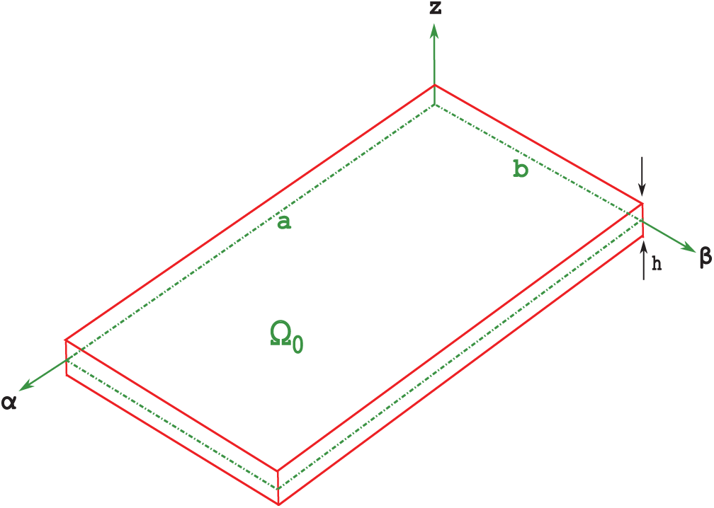
Figure 1: Plate (flat panel) geometry. Dotted green lines represent the
2.2 Geometrical and Constitutive Equations for the Magneto-Electro-Elastic Plate Problem
Geometrical equations are employed to link displacements with strains, the electric potential with the electric field and the magnetic potential with the magnetic field. MEE geometrical relations are:
where
Constitutive equations are employed to link stresses, the electric displacement and the magnetic induction with strains, electric field components and magnetic field components. Their explicit form is:
where
The solution methodology for the 3D magneto-electro-elastic free vibration problem (Eq. (1a)) is here discussed in depth. The present methodology is based on a closed-form solution. Therefore, the following coefficients have to be imposed to zero:
The imposition suggested in Eq. (8) permits the analysis of only
Navier harmonic forms for primary variables are introduced in the planar directions of the plate as follows:
where terms written in capital letters are primary variable amplitudes.
considering
Harmonic forms proposed in Eq. (10a) automatically satisfy simply supported boundary conditions for each side belonging to flat panels:
Navier harmonic forms allows to write the 3D set of second-order differential magneto-electro-elastic equations in terms of primary variable amplitudes and related first and second derivatives in
where each
The exponential matrix method is used as a solution in the
Eq. (14a) are solved via the exponential matrix method. Coefficients
Matrix form of Eq. (14a) is:
where
where
Interlaminar continuity conditions for primary variables, transverse normal and transverse shear stresses (
Interlaminar continuity conditions are imposed as:
The introduction of Eqs. (5a)–(7a) and (10a) in Eq. (17) allows interlaminar continuity conditions written in terms of maximum amplitudes:
The matrix form is:
where
The recursive introduction of Eq. (16) in Eq. (19) allows the solution along the
where
Load boundary conditions for open-circuit and closed-circuit configurations are:
The open-circuit configuration may be explicitly stated as:
The closed-circuit configuration can be explicity written as:
Both open and closed circuit conditions can be further compacted in matrix form as:
where
The null space of matrix
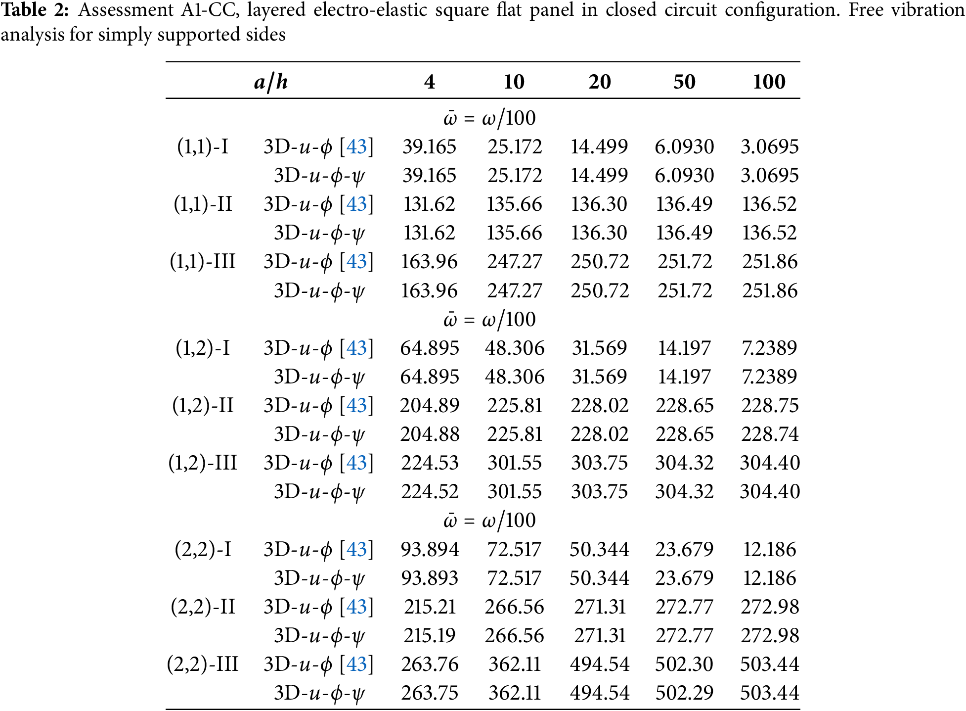
The results section is made up of two subsections. In the first one, two assessment cases are shown to validate the present 3D coupled magneto-electro-elastic model (called 3D-u-
The 3D-u-
In the benchmark subsection, a multilayered square flat panel is analyzed under open-circuit and closed-circuit conditions. The first five circular frequencies
In the first two proposed assessments, the magnetic permittivity coefficients

The first assessment (A1) considers a simply supported multilayered square flat panel with in-plane dimensions

In the second assessment (A2), a simply supported multilayered square flat panel is considered. In-plane dimensions are

In the assessment number three (A3), a simply supported three-layered thick square flat panel is considered. Geometrical dimensions are

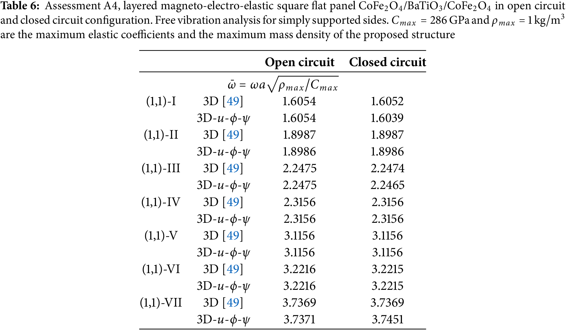
In the fourth assessment (A4), a simply supported three-layered thick square flat panel is presented considering both open and closed circuit cases. Geometrical dimensions, half-wave couples
The results proposed in all these assessments have been obtained with an order
In this benchmark subsection, the magnetic permittivity coefficients
The proposed benchmark considers a multilayered square flat panel embedding external skins made of Adaptive wood and an internal composite laminated core with stacking sequence /

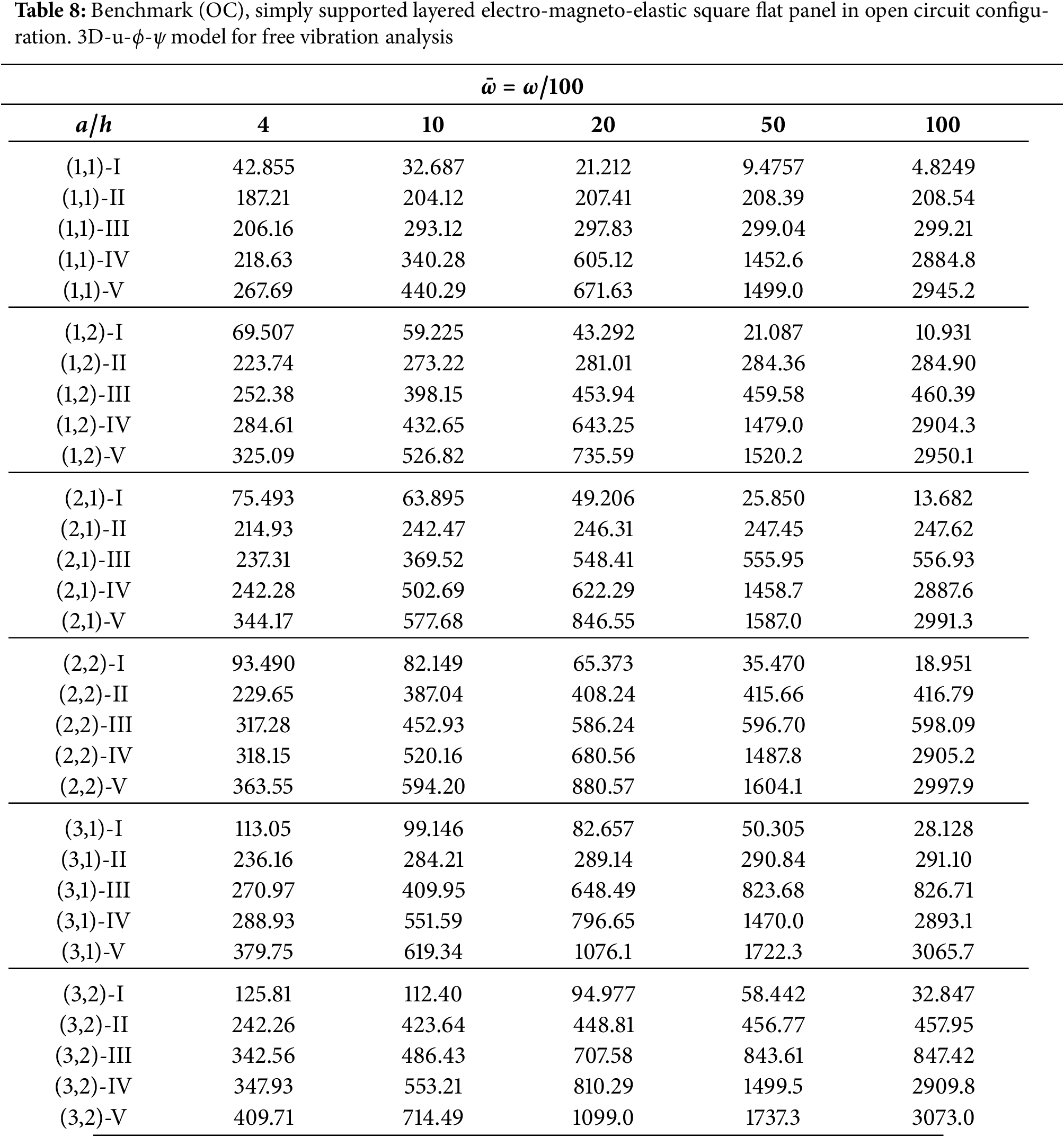
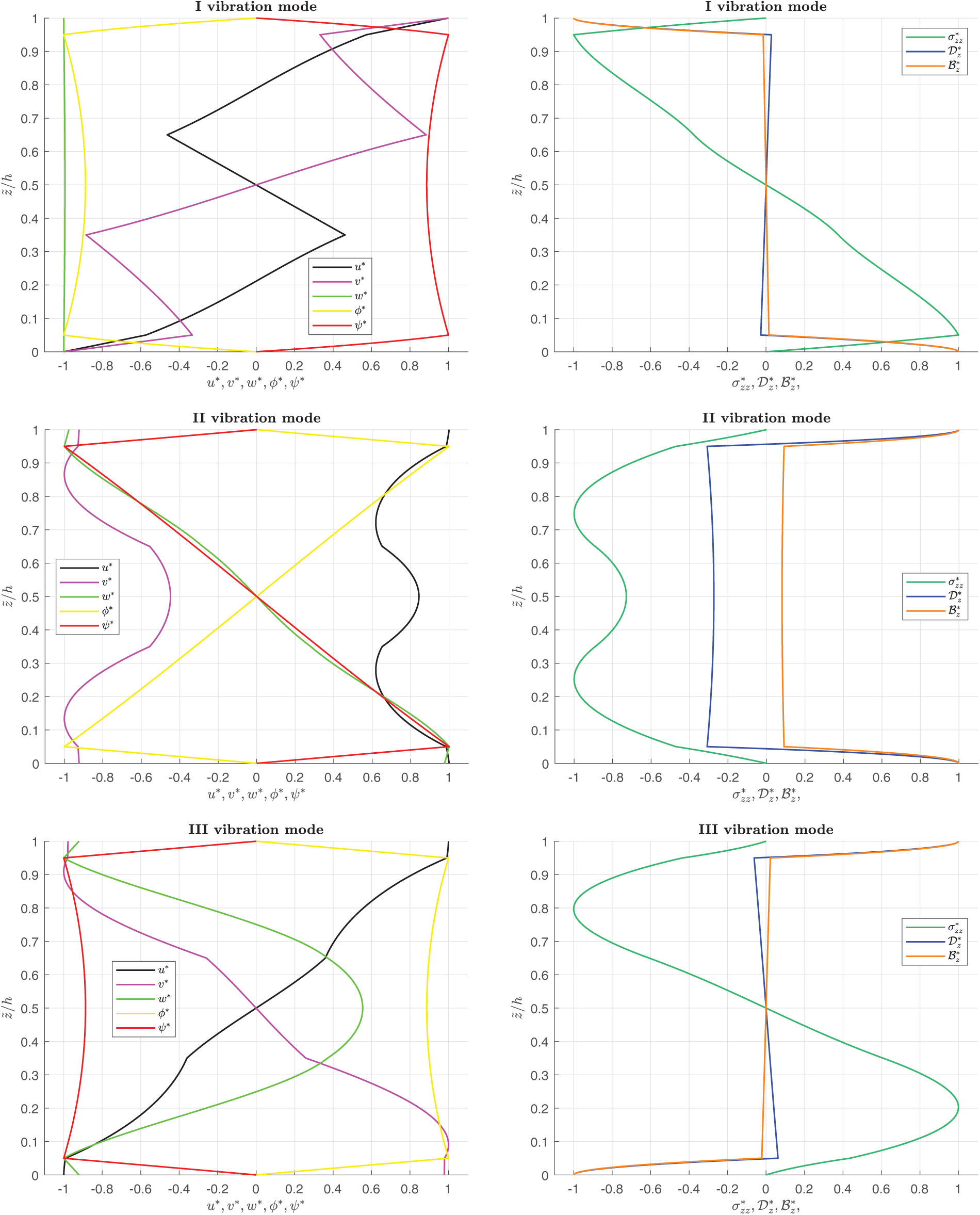
Figure 2: Benchmark (CC), simply-supported layered square flat panel in closed circuit configuration. Thickness ratio
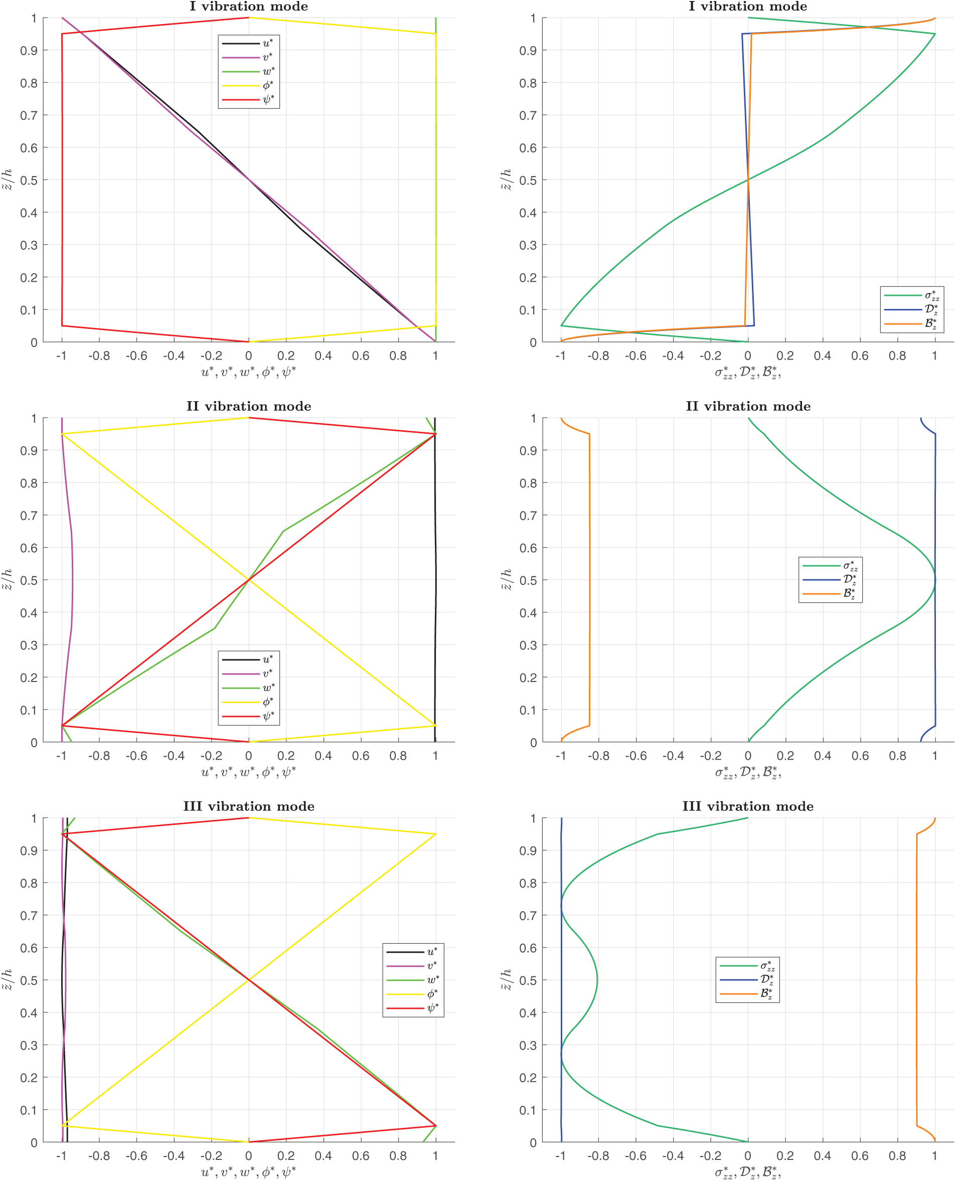
Figure 3: Benchmark (CC), simply-supported layered square flat panel in closed circuit configuration. Thickness ratio
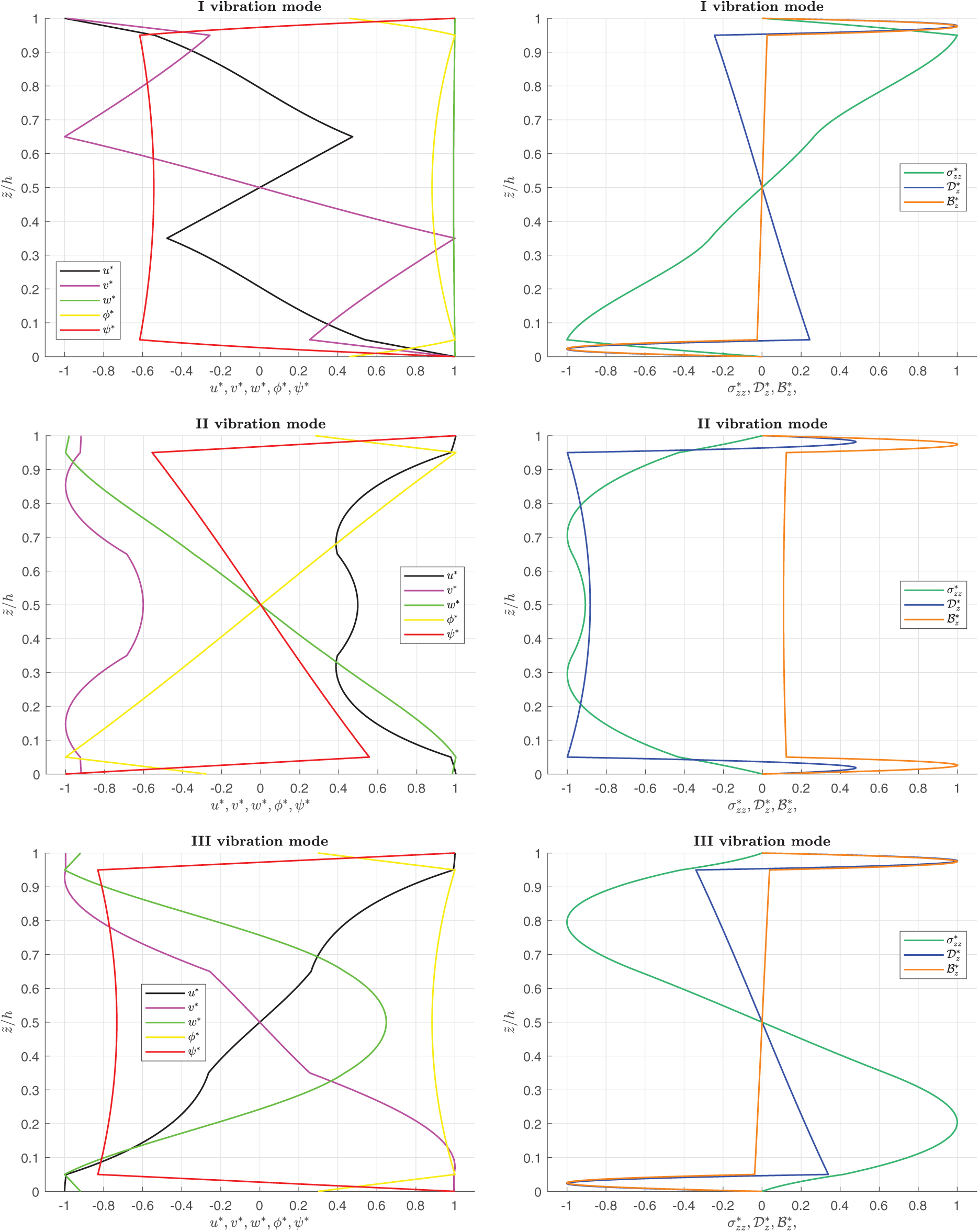
Figure 4: Benchmark (OC), simply-supported layered square flat panel in open circuit configuration. Thickness ratio
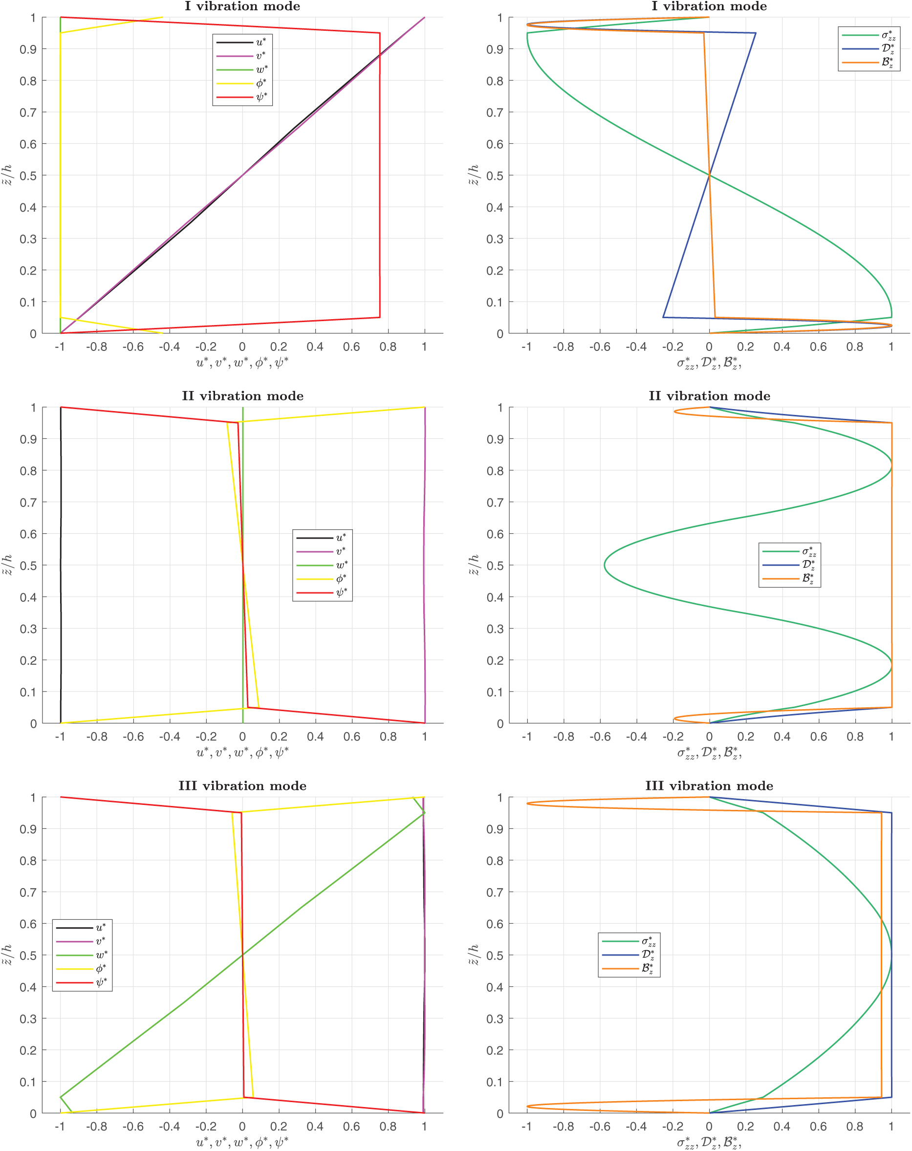
Figure 5: Benchmark (OC), simply-supported layered square flat panel in open circuit configuration. Thickness ratio
The present paper shows a 3D analytical formulation, which couples magnetic, electric and elastic fields for the free vibration analysis of simply supported flat panels. The set of five second-order differential equations for plates involves the 3D equations of motion, the 3D divergence equation for the magnetic induction and the 3D divergence equation for the electric displacement. Solution method invokes the Navier harmonic forms in the planar directions and the exponential matrix method in the transverse direction. A closed-form solution is employed: simply supported constraint conditions and isotropic or orthotropic materials are required. A layer-wise approach is implemented considering interlaminar continuity conditions in correspondence of two subsequent layers in terms of displacements, electric and magnetic potential, transverse shear and transverse normal stresses, transverse normal magnetic induction/electric displacement. In the assessments, the present 3D magneto-electro-elastic model is validated by comparing separately the results from the 3D electro-elastic model and a 3D magneto-elastic model. Comparisons with 3D electro-magneto-elastic models are also proposed. Both open and closed-circuit configurations are validated considering different thickness ratios (from thick to thin structures) and different half-wave number couples. Assessments allow the validation of the electro-elastic coupling, the magneto-elastic coupling and the electro-magneto-elastic coupling. In the new benchmark, a new plate case is proposed where the full coupling between magnetic, electric and elastic fields is considered. Circular frequency values in open and closed circuit configurations are collected in tabular form for different thickness ratios, half-wave numbers, and vibration mode orders. Circular frequencies decrease when the plate is thinner. The frequency values increase from the first to the fifth mode when the half-wave number couple is fixed. The frequency increases when the half-wave numbers increase for a given vibration mode. The open circuit configuration always gives frequency values bigger than the closed circuit configuration, even if these differences are very small. In figures for vibration modes through the thickness direction, the zigzag effect and the interlaminar continuity (connected with the transverse anisotropy) are clearly shown. Moreover, the model can correctly consider the boundary conditions related to the free vibration analysis for both open and closed circuit configurations. Future developments will consider the addition of thermal and hygroscopic fields to the proposed three-field model.
Acknowledgement: Not applicable.
Funding Statement: The authors received no specific funding for this study.
Author Contributions: The authors confirm contribution to the paper as follows: Conceptualization, Salvatore Brischetto and Domenico Cesare; methodology, Salvatore Brischetto; software, Tommaso Mondino; validation, Tommaso Mondino; formal analysis, Domenico Cesare and Tommaso Mondino; investigation, Domenico Cesare and Tommaso Mondino; resources, Salvatore Brischetto; data curation, Tommaso Mondino; writing—original draft preparation, Domenico Cesare; writing—review and editing, Salvatore Brischetto; visualization, Domenico Cesare; supervision, Salvatore Brischetto; project administration, Salvatore Brischetto; funding acquisition, Salvatore Brischetto. All authors reviewed the results and approved the final version of the manuscript.
Availability of Data and Materials: Not applicable.
Ethics Approval: Not applicable.
Conflicts of Interest: The authors declare no conflicts of interest to report regarding the present study.
Meaning of
References
1. Tornabene F. Hygro-thermo-magneto-electro-elastic theory of anisotropic doubly-curved shells. In: Higher-order strong andweak formultions for arbitrarily shaped shell structures. Bologna, Italy: Società Editrice Esculapio; 2023. [Google Scholar]
2. Zhu X. Piezoelectric ceramic materials processing, properties, characterization and applications, materials science and technologies. 1st. Hauppauge, NY, USA: Nova Science Publishers; 2010. [Google Scholar]
3. Mi X, Zhao Y, Zhan Q, Chen M. Vibration reduction study of a simplified floating raft system by installing connecting nonlinear spring-mass systems. Thin-Walled Struct. 2025;210(3):113015. doi:10.1016/j.tws.2025.113015. [Google Scholar] [CrossRef]
4. Wang S, He J, Fan J, Sun P, Wang D. A time-domain method for free vibration responses of an equivalent viscous damped system based on a complex damping model. J Low Frequency Noise Vib Active Control. 2023;42(3):1531–40. doi:10.1177/14613484231157514. [Google Scholar] [CrossRef]
5. Zhai Y, Li S, Zhang X. Vibration performance of composite doubly curved shells embedded with damping layer. Int J Struct Stab Dyn. 2025. doi:10.1142/S0219455426502652. [Google Scholar] [CrossRef]
6. Zhang X, Liu Y, Chen X, Li Z, Su C-Y. Adaptive pseudoinverse control for constrained hysteretic nonlinear systems and its application on dielectric elastomer actuator. IEEE/ASME Trans Mechatron. 2023;28(4):2142–54. doi:10.1109/tmech.2022.3231263. [Google Scholar] [CrossRef]
7. Ren H, Zhuang X, Rabczuk T. Nonlocal operator method with numerical integration for gradient solid. Comput Struct. 2020;233(1):106235. doi:10.1016/j.compstruc.2020.106235. [Google Scholar] [CrossRef]
8. Carrera E, Gifico MDi, Nali P, Brischetto S. Refined multilayered plate elements for coupled magneto-electro-elastic analysis. Multidiscip Model Mater Struct. 2009;5(2):119–38. doi:10.1163/157361109787959859. [Google Scholar] [CrossRef]
9. Yang ZX, Dang PF, Han QK, Jin ZH. Natural characteristics analysis of magneto-electro-elastic multilayered plate using analytical and finite element method. Compos Struct. 2018;185(3):411–20. doi:10.1016/j.compstruct.2017.11.031. [Google Scholar] [CrossRef]
10. Bhangale RK, Ganesan N. Free vibration of simply supported functionally graded and layered magneto-electro-elastic plates by finite element method. J Sound Vib. 2006;294(4–5):1016–38. doi:10.1016/j.jsv.2005.12.030. [Google Scholar] [CrossRef]
11. Chen JY, Heyliger PR, Pan E. Free vibration of three-dimensional multilayered magneto-electro-elastic plates under combined clamped/free boundary conditions. J Sound Vib. 2014;333(17):4017–29. doi:10.1016/j.jsv.2014.03.035. [Google Scholar] [CrossRef]
12. Jiangong Y, Juncai D, Zhijuan M. On dispersion relations of waves in multilayered magneto-electro-elastic plates. Appl Math Model. 2012;36(12):5780–91. doi:10.1016/j.apm.2012.01.028. [Google Scholar] [CrossRef]
13. Pham Q-H, Tran VK, Nguyen P-C. Dynamic response of magneto-electro-elastic composite plates lying on visco-Pasternak medium subjected to blast load. Compos Struct. 2024;337:118054. doi:10.1016/j.compstruct.2024.118054. [Google Scholar] [CrossRef]
14. Kattimani SC, Ray MC. Smart damping of geometrically nonlinear vibrations of magneto-electro-elastic plates. Compos Struct. 2014;114(5):51–63. doi:10.1016/j.compstruct.2014.03.050. [Google Scholar] [CrossRef]
15. Xu LL, Kang CC, Zheng YF, Chen CP. Analysis of nonlinear vibration of magneto-electro-elastic plate on elastic foundation based on high-order shear deformation. Compos Struct. 2021;271:114149. doi:10.1016/j.compstruct.2021.114149. [Google Scholar] [CrossRef]
16. Vinyas M. A higher-order free vibration analysis of carbon nanotube-reinforced magneto-electro-elastic plates using finite element methods. Compos Part B Eng. 2019;158(4):286–301. doi:10.1016/j.compositesb.2018.09.086. [Google Scholar] [CrossRef]
17. Milazzo A. Variable kinematics models and finite elements for nonlinear analysis of multilayered smart plates. Compos Struct. 2015;122(1):537–45. doi:10.1016/j.compstruct.2014.12.003. [Google Scholar] [CrossRef]
18. Milazzo A. Refined equivalent single layer formulations and finite elements for smart laminates free vibrations. Compos Part B Eng. 2014;61(16):238–53. doi:10.1016/j.compositesb.2014.01.055. [Google Scholar] [CrossRef]
19. Milazzo A. An equivalent single-layer approach for free vibration analysis of smart laminated thick composite plates. Smart Mater Struct. 2012;21:075031. [Google Scholar]
20. Davì G, Milazzo A. A regular variational boundary model for free vibrations of magneto-electro-elastic structures. Eng Anal Bound Elem. 2011;35(3):303–12. doi:10.1016/j.enganabound.2010.10.004. [Google Scholar] [CrossRef]
21. Vinyas M, Kattimani SC. Finite element evaluation of free vibration characteristics of magneto-electro-elastic rectangular plates in hygrothermal environment using higher-order shear deformation theory. Compos Struct. 2018;202(3):1339–52. doi:10.1016/j.compstruct.2018.06.069. [Google Scholar] [CrossRef]
22. Ramirez F, Heyliger PR, Pan E. Free vibration response of two-dimensional magneto-electro-elastic laminated plates. J Sound Vib. 2006;292(3–5):626–44. doi:10.1016/j.jsv.2005.08.004. [Google Scholar] [CrossRef]
23. Kiran MC, Kattimani SC. Free vibration of multilayered magneto-electro-elastic plates with skewed edges using layer wise shear deformation theory. Mater Today Proc. 2018;5(10):21248–21255. doi:10.1016/j.matpr.2018.06.525. [Google Scholar] [CrossRef]
24. Soni S, Jain NK, Joshi PV. Analytical modeling for nonlinear vibration analysis of partially cracked thin magneto-electro-elastic plate coupled with fluid. Nonlinear Dyn. 2017;90(1):137–70. doi:10.1007/s11071-017-3652-5. [Google Scholar] [CrossRef]
25. Xu L-L, Chen C-P, Zheng Y-F. Two-degrees-of-freedom nonlinear free vibration analysis of magneto-electro-elastic plate based on high order shear deformation theory. Commun Nonlinear Sci Numer Simul. 2022;114:106662. doi:10.1016/j.cnsns.2022.106662. [Google Scholar] [CrossRef]
26. Yang Y, Li X-F. Bending and free vibration of a circular magnetoelectroelastic plate with surface effects. Int J Mech Sci. 2019;157–158(1):858–71. doi:10.1016/j.ijmecsci.2019.05.029. [Google Scholar] [CrossRef]
27. Chen J, Chen H, Pan E, Heyliger PR. Modal analysis of magneto-electro-elastic plates using the state-vector approach. J Sound Vib. 2007;304(3–5):722–34. doi:10.1016/j.jsv.2007.03.021. [Google Scholar] [CrossRef]
28. Chen J, Pan E, Chen H. Wave propagation in magneto-electro-elastic multilayered plates. Int J Solids Strct. 2007;44(3–4):1073–85. doi:10.1016/j.ijsolstr.2006.06.003. [Google Scholar] [CrossRef]
29. Chen J, Guo J, Pan E. Wave propagation in magneto-electro-elastic multilayered plates with nonlocal effect. J Sound Vib. 2017;400:550–63. doi:10.1016/j.jsv.2017.04.001. [Google Scholar] [CrossRef]
30. Pan E, Heyliger PR. Free vibrations of simply supported and multilayered magneto-electro-elastic plates. J Sound Vib. 2002;252(3):429–42. doi:10.1006/jsvi.2001.3693. [Google Scholar] [CrossRef]
31. Dat ND, Quan TQ, Vinyas M, Nguyen DD. Analytical solutions for nonlinear magneto-electro-elastic vibration of smart sandwich plate with carbon nanotube reinforced nanocomposite core in hygrothermal environment. Int J Mech Sci. 2020;186:105906. doi:10.1016/j.ijmecsci.2020.105906. [Google Scholar] [CrossRef]
32. Wang J, Qu L, Qian F. State vector approach of free-vibration analysis of magneto-electro-elastic hybrid laminated plates. Compos Struct. 2010;92(6):1318–24. doi:10.1016/j.compstruct.2009.11.013. [Google Scholar] [CrossRef]
33. Razavi S, Shooshtari A. Nonlinear free vibration of magneto-electro-elastic rectangular plates. Compos Struct. 2015;119(3):377–84. doi:10.1016/j.compstruct.2014.08.034. [Google Scholar] [CrossRef]
34. Xin L, Hu Z. Free vibration of simply supported and multilayered magneto-electro-elastic plates. Compos Struct. 2015;121(6):344–50. doi:10.1016/j.compstruct.2014.11.030. [Google Scholar] [CrossRef]
35. Kuo H-Y, Wang Y-H. Wave motion of magneto-electro-elastic laminated plates with membrane-type interfacial imperfections. Compos Struct. 2022;293:115661. doi:10.1016/j.compstruct.2022.115661. [Google Scholar] [CrossRef]
36. Dinh KN, Duc TV. Vibration analysis of a magneto-electro-elastic sandwich composite plate with a new honeycomb structure core layer in a thermal environment. Aerosp Sci Technol. 2025;157(3):109846. doi:10.1016/j.ast.2024.109846. [Google Scholar] [CrossRef]
37. Hamidi M, Zaki S, Aboussaleh M. Modeling and numerical simulation of the dynamic behavior of magneto-electro-elastic multilayer plates based on aWinkler-Pasternak elastic foundation. J Intell Mater Syst Struct. 2020;32(8):1–15. doi:10.1177/1045389x20969845. [Google Scholar] [CrossRef]
38. Ke L-L, Wang Y-S, Yang J, Kitipornchai S. Free vibration of size-dependent magneto-electro-elastic nanoplates based on the nonlocal theory. Acta Mech Sin. 2014;30(4):516–25. doi:10.1007/s10409-014-0072-3. [Google Scholar] [CrossRef]
39. Li YS, Cai ZY, Shi SY. Buckling and free vibration of magnetoelectroelastic nanoplate based on nonlocal theory. Compos Struct. 2014;111:522–9. doi:10.1016/j.compstruct.2014.01.033. [Google Scholar] [CrossRef]
40. Chang T-P. Free vibration of fluid-loaded transversely isotropic magneto-electro-elastic plates. Appl Mech Mater. 2013;284–287:758–62. doi:10.4028/www.scientific.net/amm.284-287.758. [Google Scholar] [CrossRef]
41. Jamalpoor A, Ahmadi-Savadkoohi A, Hosseini-Hashemi S. Free vibration and biaxial buckling analysis of magneto-electro-elastic microplate resting on visco-Pasternak substrate via modified strain gradient theory. Smart Mater Struct. 2016;25(10):105035. doi:10.1088/0964-1726/25/10/105035. [Google Scholar] [CrossRef]
42. Shooshtari A, Razavi S. Vibration of a multiphase magneto-electro-elastic simply supported rectangular plate subjected to harmonic forces. J Intell Mater Syst Struct. 2016;28(4):451–67. doi:10.1177/1045389x16649451. [Google Scholar] [CrossRef]
43. Brischetto S, Cesare D. Three-dimensional vibration analysis of multilayered composite and functionally graded piezoelectric plates and shells. Compos Struct. 2024;346(1):118413. doi:10.1016/j.compstruct.2024.118413. [Google Scholar] [CrossRef]
44. Brischetto S, Cesare D. A 3D shell model for static and free vibration analysis of multilayered magneto-elastic structures. Thin-Walled Struct. 2025;206(7):112620. doi:10.1016/j.tws.2024.112620. [Google Scholar] [CrossRef]
45. Brischetto S. An exact 3D solution for free vibrations of multilayered cross-ply composite and sandwich plates and shells. Int J Appl Mech. 2014;6(6):1450076. doi:10.1142/s1758825114500768. [Google Scholar] [CrossRef]
46. Povstenko Y. Fractional thermoelasticity. Cham, Switzerland: Springer International Publishing; 2015. [Google Scholar]
47. Boyce WE, DiPrima RC. Elementary differential equations and boundary value problems. New York, NY, USA: John Wiley & Sons, Ltd.; 2001. [Google Scholar]
48. Reddy JN. Mechanics of laminated composite plates and shells. In: Theory and analysis. Boca Raton, FL, USA: CRC Press; 2014. [Google Scholar]
49. Chen WQ, Lee KY, Ding HJ. On free vibration of non-homogeneous transversely isotropic magneto-electro-elastic plates. J Sound Vib. 2005;279(1–2):237–51. doi:10.1016/j.jsv.2003.10.033. [Google Scholar] [CrossRef]
50. Pan E. Three-dimensional Green’s functions in anisotropic magneto-electro-elastic bimaterials. Zeitschrift Fur Angewandte Mathematik Und Physik ZAMP. 2002;53:815–38. [Google Scholar]
Cite This Article
 Copyright © 2025 The Author(s). Published by Tech Science Press.
This work is licensed under a Creative Commons Attribution 4.0 International License , which permits unrestricted use, distribution, and reproduction in any medium, provided the original work is properly cited.
 Downloads
 Citation Tools