Subdivision-Based Isogeometric BEM with Deep Neural Network Acceleration for Acoustic Uncertainty Quantification under Ground Reflection Effects

1  Introduction

Noise control remains a central concern in both civil and defense engineering applications. Among various strategies aimed at mitigating acoustic radiation, such as controlling noise at the source or along propagation paths, the integration of sound-absorbing materials on structural surfaces has proven to be a particularly pragmatic and cost-effective solution. This approach enables attenuation of radiated sound without necessitating geometric modifications to the original structure.

In practice, however, the performance of these sound-absorbing treatments is subject to uncertainty arising from environmental and material-related factors. Variation in surface impedance, temperature fluctuations, and ground reflection conditions can all introduce stochastic behavior into the acoustic response of a system [1–3]. To reliably evaluate the robustness of such treatments under real-world conditions, rigorous uncertainty quantification (UQ) techniques are essential [4,5].

Among the existing methods for stochastic analysis, Monte Carlo simulations (MCs) [6–8] remain a benchmark due to their conceptual simplicity and wide applicability. Their reliance on statistical sampling makes them model-agnostic, which is especially advantageous in the context of nonlinear or high-dimensional problems. However, the computational expense of MCs is often prohibitive when applied to large-scale systems or high-fidelity solvers, as thousands of simulations may be required to obtain statistically meaningful results.

The boundary element method (BEM) [9,10] is particularly attractive for exterior acoustic problems, owing to its dimensional reduction property: only the surface of the domain requires discretization. In contrast to volumetric methods such as the finite element method (FEM) [11–14], BEM offers exact treatment of radiation conditions at infinity and is therefore well-suited for acoustic scattering analysis. Nevertheless, the accuracy of BEM solutions is contingent on the quality of the surface mesh [15].

Recent advances in geometric modeling have introduced subdivision surface schemes that offer smooth representations of complex geometries. Specifically, the Catmull-Clark subdivision method [16,17] has demonstrated compatibility with isogeometric BEM formulations. When combined with BEM, subdivision surfaces enhance geometric fidelity and allow for seamless mesh refinement. Various spline-based techniques—such as NURBS [18–20], T-splines [21,22], and PHT-splines [23,24]—have further bridged the gap between CAD and numerical analysis.

However, as model complexity increases, so too does the number of mesh elements and degrees of freedom, leading to considerable computational burden. This challenge is further compounded in UQ, where thousands of simulations may be needed to capture the system’s stochastic behavior. Accordingly, there is a pressing need for strategies that can accelerate sample generation without compromising accuracy.

In recent years, the integration of machine learning into scientific computing has emerged as a promising solution. Unlike classical surrogate modeling techniques—such as Gaussian process regression [25–27], polynomial chaos expansion [28–30], radial basis functions [5,31], or relevance vector machines [32]—deep neural networks (DNNs) exhibit superior scalability and approximation capacity in high-dimensional, nonlinear settings. Recent works [33–35] have demonstrated their utility in learning complex mappings from uncertain parameters to physical responses. Farajollahi et al. [36,37] employed deep neural networks to efficiently predict and perform inverse design of dispersion bandgaps in cylindrically pillared acoustic metamaterials, while analyzing the model’s sensitivity to each geometric parameter using Shapley values. In addition, they used a deep neural network to predict bandgap characteristics and ratios in columnar phononic crystals, achieving high accuracy and revealing the influence of geometric parameters through shapley values. Moreover, the incorporation of physics-informed constraints [38–40] has improved the interpretability and robustness of such models.

In this work, we propose a DNN-accelerated framework for acoustic uncertainty analysis. The method combines Catmull-Clark subdivision surfaces for geometry representation, BEM for forward acoustic simulation, and DNNs for efficient surrogate modeling. Our objective is to achieve high-fidelity simulation results while dramatically reducing the computational cost of uncertainty propagation.

The rest of this paper is organized as follows. Section 2.1 presents the Catmull-Clark subdivision surface technique used for mesh generation. Section 2.2 outlines the BEM formulation for the Helmholtz equation with sound-absorbing boundaries and ground reflection. Section 4 introduces the DNN-based surrogate model and training methodology. Section 5 validates the proposed approach via numerical examples, and Section 6 summarizes the conclusions.

2  Computational Modeling and Acoustic Field Analysis

2.1 Mesh Generation Methods Using Catmull-Clark Subdivision

Subdivision surfaces offer a robust geometric discretization framework for generating smooth and continuous representations of arbitrarily complex topologies. Originating from B-spline curve formulations, these techniques iteratively refine a coarse control mesh to approach a smooth limit surface. The refinement process typically involves two key operations: (1) insertion of new vertices and redefinition of topological connectivity, and (2) recalculation of vertex positions. This process is repeated until geometric convergence is achieved.

In high-fidelity numerical simulation, particularly in isogeometric analysis (IGA) [41–43], it is essential to maintain geometric smoothness and basis function continuity across elements. Traditional FEM/BEM implementations rely on polynomial basis functions, whereas IGA unifies geometric modeling and numerical approximation by employing identical basis functions for both geometry and solution fields. This consistency enables accurate modeling of high-order continuous fields and facilitates applications involving Kirchhoff–Love shell formulations.

Although NURBS are commonly used in CAD and IGA, they face limitations in topological flexibility and watertightness. To address these challenges, this work adopts Catmull-Clark subdivision surfaces in place of NURBS. The Catmull-Clark approach supports arbitrary topologies while ensuring C1 continuity and watertight surface representations.

The procedure begins by constructing a quadrilateral control mesh, where each corner defines a control point (Fig. 1). At each subdivision level k, a new set of control points is computed, and the original ones are repositioned. This recursive refinement from level k to k+1 employs predefined weighting schemes for edge points (E-points), face points (F-points), and vertex points (V-points), as shown in Fig. 2. The updated coordinates for each point type are computed using the following expressions:

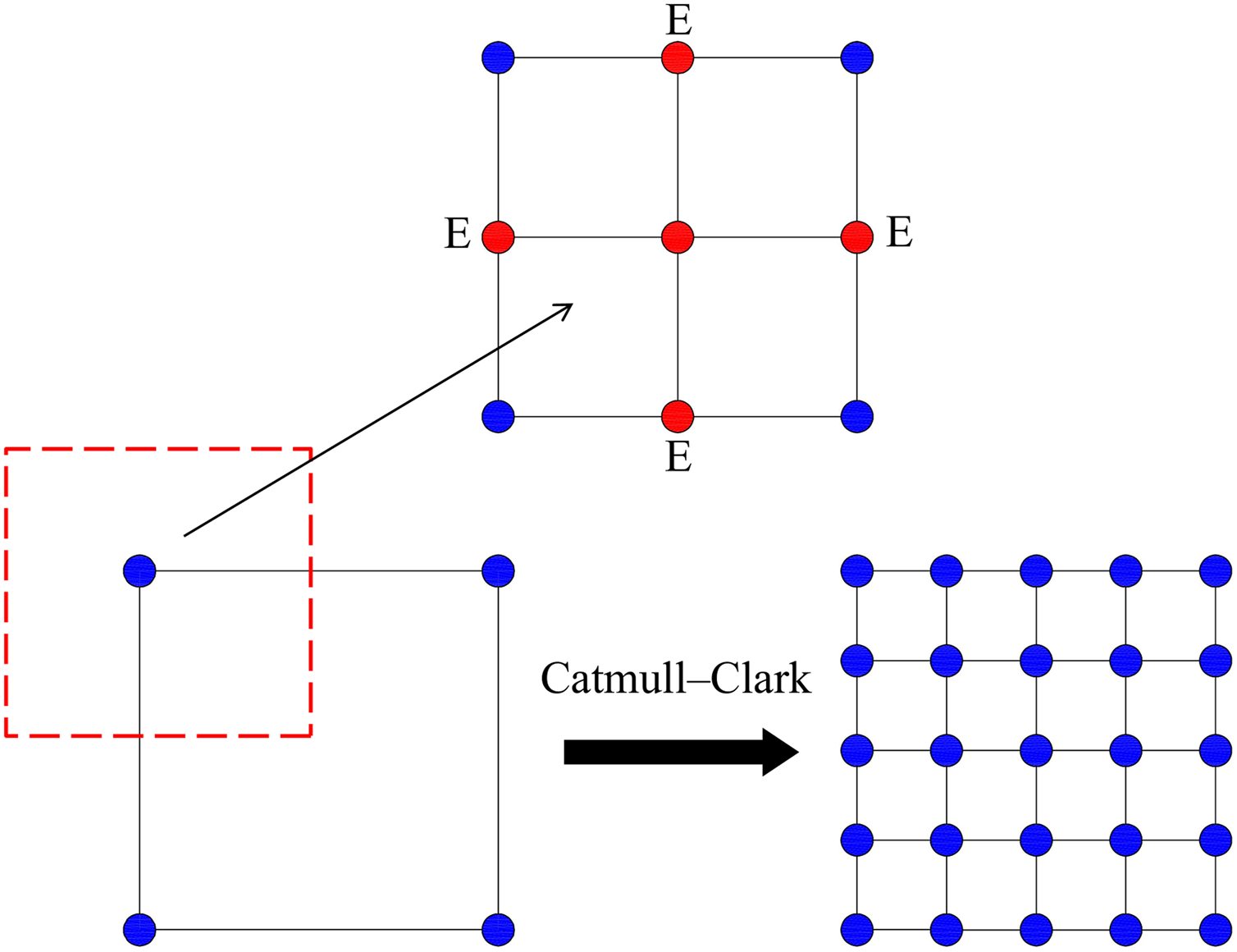
Figure 1: The Catmull-Clark subdivision process

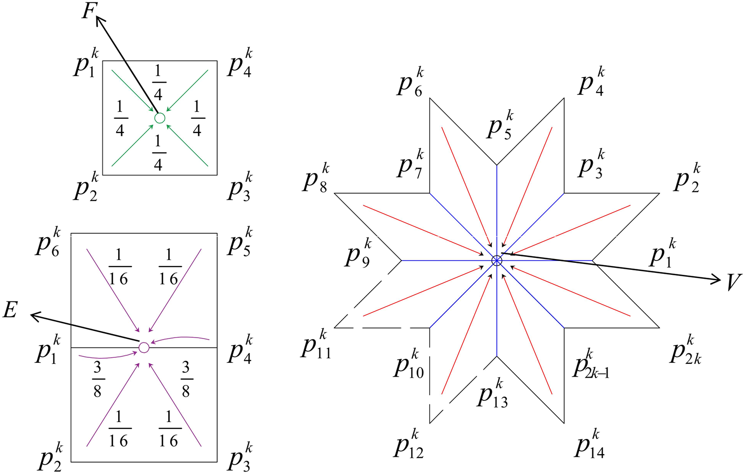
Figure 2: Multi-level subdivision process

E-point:

pek+1=38(p1k+p4k)+116(p2k+p3k+p5k+p6k)(1)

where p1,p2,p3,p4,p5,p6 are the vertices of the two adjacent quadrilateral elements sharing the edge where E-point is located.

F-point:

pfk+1=14(p1k+p2k+p3k+p4k)(2)

where p1,p2,p3,p4 are the four vertices of a quadrilateral element where F-point is located.

V-point:

pvk+1=γpivk+αv∑i=1kp2ik+βv∑i=1kp2i−1k(3)

where α=32v, β=14v, and γ=1−α−β. pvk denotes the original vertex, and its 1-ring neighboring vertices be p1,p2,…,p2k.

It is important to note that the subdivision process cannot be applied indefinitely. Instead, convergence toward a smooth limit surface is evaluated based on the properties of the underlying spline basis functions. As subdivision progresses, the mesh becomes increasingly regular in regions distant from extraordinary vertices (i.e., vertices with valence different from four). In the vicinity of such extraordinary points, local irregularities persist in early subdivision stages, but the structure eventually transitions to a quasi-regular configuration with continued refinement.

Once this convergence behavior is understood, it becomes possible to derive analytical expressions for the geometric properties of the limit surface, even near extraordinary vertices. Stam [44] introduced a closed-form formulation for evaluating Catmull-Clark subdivision surfaces at arbitrary parametric locations, which facilitates accurate geometric and derivative evaluations.

In this work, we adopt a matrix-based representation of the subdivision process. Let pk and pk+1 denote the vectors of vertex coordinates at levels k and k+1, respectively. The refinement operation can then be compactly written as:

pk+1=Spk(4)

where S is the global subdivision matrix, whose entries encode the refinement rules for all vertex types (face, edge, and vertex points).

A key advantage of Catmull-Clark subdivision surfaces is their ability to ensure C1 continuity and smooth curvature, even across irregular topologies. In cases where all mesh vertices have valence 4, the mesh is considered regular and yields uniform subdivision. Vertices with valence other than 4 introduce irregularities, as illustrated in Fig. 3, where a colored element contains an extraordinary vertex. To handle such cases, repeated subdivision is applied until the region becomes sufficiently regular for accurate approximation. Ultimately, the point of interest falls within a patch that can be described using known subdivision basis functions and associated control points.

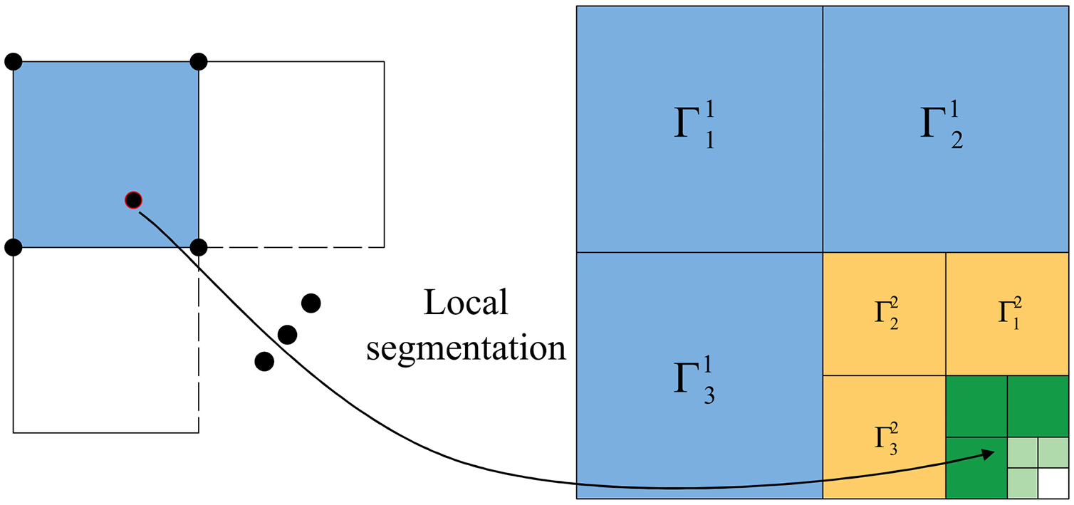
Figure 3: Local subdivision process

After sufficient refinement, the surface position at any parametric coordinate (ξ,η) can be expressed as:

x(ξ,η)=∑ℓ=02κN^ℓ(ξ,η)Pℓ(5)

Here, κ is the valence of the central vertex, N^ℓ is the subdivision basis functions, and Pℓ is the associated control points. Detailed expressions for N^ℓ can be found in Chen’s work [45].

2.2 Acoustic Field Analysis Using IGA-BEM

The propagation of time-harmonic acoustic waves in a homogeneous fluid domain is governed by the Helmholtz equation:

∇2p(x)+k2p(x)=0,∀x∈Ω,(6)

where p(x) denotes the acoustic pressure at spatial location x, ∇2 is the Laplacian operator, k=ω/c is the acoustic wave number, ω is the angular frequency, and c is the speed of sound in the medium.

To avoid volumetric meshing and ensure accurate enforcement of radiation conditions, we employ the boundary element method (BEM), which reformulates Eq. (6) into an equivalent boundary integral equation. For a field point x∈Γ, the boundary integral representation reads:

C(x)p(x)−∫ΓG(x,y)q(y)dΓ(y)+∫Γ∂G(x,y)∂nf(y)p(y)dΓ(y)=pinc(x),(7)

where y denotes the source point on the boundary Γ, G(x,y) is the free-space Green’s function, q(y)=∂p/∂nf is the normal derivative of pressure (i.e., acoustic flux), and C(x)=1/2 for smooth boundaries.

When sound-absorbing materials are applied to the structure, the impedance boundary condition is given by:

q(y)=ikβ(y)p(y),(8)

where β(y) is the normalized acoustic admittance at point y. Substituting this condition into Eq. (7) leads to a single-variable integral equation in p(y).

The fundamental solution (Green’s function) and its normal derivative in three-dimensional free space are given by:

G(x,y)=eikr4πr,(9)

∂G(x,y)∂nf(y)=−eikr4πr2(1−ikr)∂r∂nf(y),(10)

where r=|x−y| denotes the Euclidean distance.

To incorporate ground reflection effects, a half-space fundamental solution is used:

F(x,y)=G(x,y)+β1G(x,y∗),(11)

where y∗ is the mirror image of y across the ground plane, and β1∈[−1,1] is a reflection coefficient: β1=1 corresponds to a perfectly rigid surface, while β1=−1 denotes a perfectly soft (absorptive) surface.

Replacing G(x,y) with F(x,y) in Eq. (7), and applying the Burton–Miller formulation to improve numerical robustness, we obtain:

C(x)p(x)+αC(x)ikβ~p(x)=∫ΓF(x,y)ikβ~p(y)dΓ+α∫Γ∂F(x,y)∂nf(x)ikβ~p(y)dΓ−∫Γ∂F(x,y)∂nf(y)p(y)dΓ−α∫Γ∂2F(x,y)∂nf(x)∂nf(y)p(y)dΓ+p~inc∗(x),(12)

where α is the coupling parameter in the Burton–Miller formulation and p~inc∗=pinc+∂pinc/∂nf.

The derivatives of F(x,y) used above are computed as:

∂F(x,y)∂nf(y)=−eikr4πr2(1−ikr)∂r∂nf(y)−β1eikr∗4π(r∗)2(1−ikr∗)∂r∗∂nf(y),(13)

∂F(x,y)∂nf(x)=−eikr4πr2(1−ikr)∂r∂nf(x)−β1eir∗4π(r∗)2(1−ikr∗)∂r∗∂nf(x),(14)

∂2F(x,y)∂nf(x)∂nf(y)=eikr4πr3[(3−3ikr−k2r2)∂r∂nf(y)∂r∂nf(x)+(1−ikr)ni(x)ni(y)]+β1eikr∗4π(r∗)3[(3−3ikr∗−k2(r∗)2)∂r∗∂nf(y)∂r∗∂nf(x)+(1−ikr∗)ni(x)ni(y)].(15)

To discretize Eq. (12) within the IGA-BEM framework, the pressure pe and its flux qe over each element e are approximated using the same subdivision basis functions N^ℓ(ξ,η) employed in the geometry:

pe(ξ,η)=∑ℓ=02κN^ℓ(ξ,η)p~ℓe,(16)

qe(ξ,η)=∑ℓ=02κN^ℓ(ξ,η)q~ℓe.(17)

Substituting these approximations into Eq. (12) and applying collocation at each point xj, the discretized system becomes:

C(xj)p(xj)+αC(xj)ikβ~p(xj)+∑e=1Ne∑ℓ=02κ∫ΓeN^ℓ(ξ,η)∂F(xj,y)∂nf(y)dΓp~ℓe+α∑e=1Ne∑ℓ=02κ∫ΓeN^ℓ(ξ,η)∂2F(xj,y)∂nf(xj)∂nf(y)dΓp~ℓe=∑e=1Ne∑ℓ=02κ∫ΓeN^ℓ(ξ,η)F(xj,y)dΓikβ~p~ℓe+α∑e=1Ne∑ℓ=02κ∫ΓeN^ℓ(ξ,η)∂F(xj,y)∂nf(xj)dΓikβ~p~ℓe+p~inc∗(xj).(18)

This system can be compactly expressed in matrix form as:

Hp~=G(ikβ~)p~+pinc,(19)

where H and G are dense coefficient matrices assembled from the boundary integrals, p~ is the vector of unknown pressure coefficients, and pinc contains the incident field terms at collocation points.

The treatment of singular and near-singular integrals arising in Eq. (18) is discussed in detail in Appendices A and Appendices B.

3  Monte Carlo Simulation

Monte Carlo simulation (MCs) is a widely used statistical technique for quantifying the effects of uncertainty and randomness in engineering systems [46,47]. In the context of the BEM-based acoustic simulation introduced in Section 2.2, the primary sources of uncertainty include the variability in the ground reflection coefficient and the acoustic properties of sound-absorbing materials. The MCs framework enables the assessment of how these stochastic input parameters influence the acoustic pressure field by repeatedly sampling from their probability distributions and evaluating the corresponding system response.

The core objective of MCs is to estimate key statistical quantities—such as the mean and standard deviation—of a physical response. These metrics serve as quantitative indicators of uncertainty and associated risks. Given N independent realizations xl of the input parameters, the statistical estimators are computed as:

E≈1N∑l=1Nf(xl),(20)

D≈1N−1∑l=1N(f(xl)−E)2,(21)

where f(xl) denotes the model response corresponding to the l-th sample, and E and D represent the estimated expectation and variance, respectively.

The general procedure for executing a Monte Carlo simulation comprises the following steps:

1.   Define the physical problem and its mathematical/numerical model, along with the relevant uncertain parameters.

2.   Generate samples from the joint probability distribution of the input variables.

3.   Evaluate the model response at each sample point to form a dataset of input–output pairs.

4.   Compute statistical metrics (e.g., mean, variance, confidence intervals) to quantify uncertainty.

Let X denote a random variable defined on the bounded domain:

X={xi∈[xmin,xmax]},i=1,…,n,(22)

and define a set of N samples as:

Xi={xl|xl∈X},l=1,…,N.(23)

Let x=[x1,…,xn]T∈Rn, and the model output corresponding to each input sample is denoted by:

Y={yl=f(xl)|xl∈X},l=1,…,N,(24)

where Y=[y1,…,ym]T∈Rm represents the output response vector. The full dataset comprising input–output pairs can then be expressed as:

{(x1,Y1),…,(xl,Yl),…,(xN,YN)}.(25)

While conceptually simple and broadly applicable, MCs are computationally intensive. The number of required samples N grows rapidly with increasing problem dimensionality and desired confidence level. Consequently, the cost of obtaining high-fidelity solutions—especially for problems involving large-scale simulations or expensive numerical solvers—can be prohibitive. This computational bottleneck becomes particularly severe when the forward model involves repeated acoustic BEM analyses or complex geometries.

Therefore, there is a pressing need for efficient acceleration strategies that reduce the computational load of MC simulations without compromising accuracy. This motivates the integration of machine learning-based surrogate models, which aim to approximate the system response with significantly reduced evaluation cost—a topic discussed in detail in Section 4.

4  DNN for Accelerated Computation

To efficiently generate large volumes of high-fidelity acoustic response data for uncertainty quantification, a deep neural network (DNN) [48–50] is employed as a surrogate model to replace repeated full-order simulations. The DNN framework significantly reduces computational cost while maintaining satisfactory prediction accuracy.

4.1 Dataset Construction and Variable Modeling

In real-world scenarios, parameters such as the sound-absorbing material properties and ground reflection coefficients exhibit variability due to environmental factors (e.g., temperature fluctuation, soil composition). To model this uncertainty, all input variables are assumed to follow Gaussian distributions. Random sampling is used to generate representative datasets, where each input variable is perturbed by a maximum variation factor of γ=0.2 to ensure physical realism and numerical stability. Table 1 summarizes the mean values and bounded perturbation ranges of the modeled parameters, using a spherical acoustic model as a case study.

Two datasets are constructed: a single-variable dataset (200 samples) and a multi-variable dataset (300 samples), with each sample corresponding to computed sound pressure levels at two target frequencies: 100 and 200 Hz. The observation point is fixed at (10, 0, 0).

4.2 Data Normalization

To improve the learning efficiency and prediction performance of the DNN, all input variables are normalized using standard score (Z-score) normalization:

zi=xi−μσ,(26)

where zi is the normalized input, xi is the raw input, and μ, σ are the mean and standard deviation of the input variable. This ensures uniform feature scaling and mitigates bias in learning due to differing magnitudes.

4.3 Neural Network Architecture and Forward Computation

The DNN architecture consists of an input layer, multiple fully connected hidden layers, and an output layer. Fig. 4 shows the network structure. The forward propagation through the DNN can be expressed as:

gj11=f(∑i=1t0wij11zil+bj11),j1=1,…,t1,gjnn=f(∑i=1tn−1wijnngin−1+bjnn),jn=1,…,tn,ykl=f(∑i=1tmwikm+1gim+bkm+1),k=1,…,tm+1,(27)

where zi, gi, and yi represent the activations of the input, hidden, and output layers, respectively. The weights w, biases b, and nonlinear activation function f collectively govern the mapping behavior of the network.

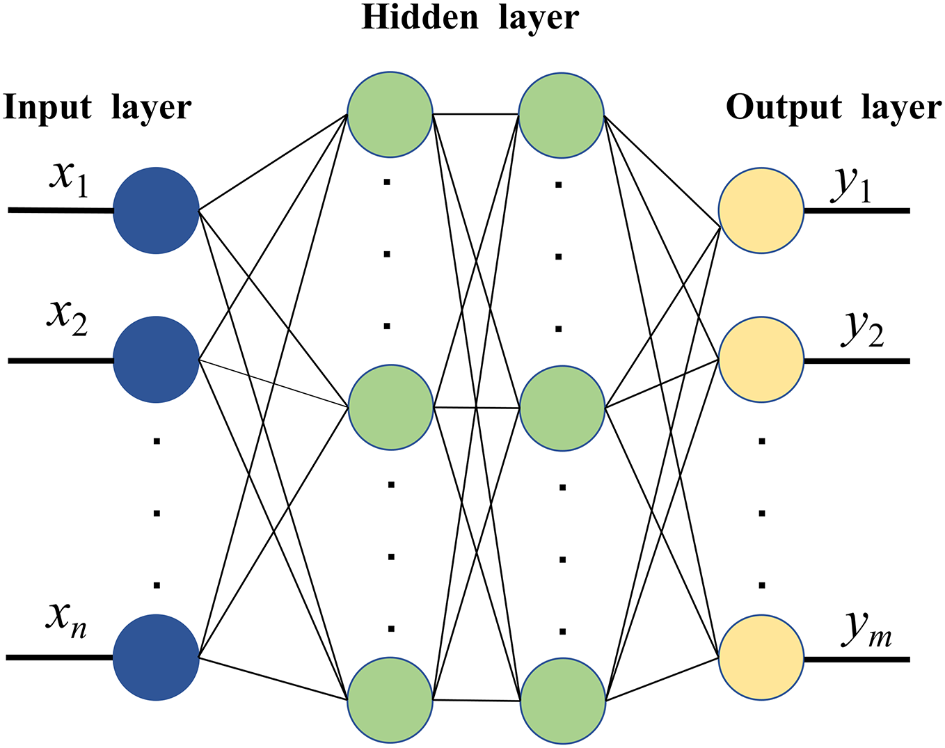
Figure 4: Architecture of the DNN surrogate model

After prediction, the inverse normalization restores results to the original physical scale:

y^ml=yml⋅σ+μ.(28)

4.4 Training Strategy and Hyperparameter Selection

The dataset is randomly split into training and testing subsets with a 9:1 ratio. The regression objective is trained using mean squared error (MSE) as the loss function:

Loss=1NI∑l=1NI∑m=1M(y^ml−yml)2,(29)

where NI is the total number of samples, M is the output dimension, and y^ml, yml are the predicted and true values.

To evaluate performance, two additional statistical metrics are used:

MAPE=1NIM∑l=1NI∑m=1M|yml−y^mlyml|×100%,(30)

R2=1−∑l=1NI∑m=1M(yml−y^ml)2∑l=1NI∑m=1M(yml−y¯)2.(31)

Table 2 summarizes the hyperparameters used in training across different input dimensionalities.

4.5 Hyperparameter Tuning and Optimizer Selection

The tuning process for single-variable input follows a sequential grid-search approach, where one hyperparameter is varied at a time. The impact of optimizer type, learning rate, number of hidden layers, and activation function is systematically assessed.

Fig. 5a compares different optimizers. Adagrad converges slowly and exhibits large fluctuations; Adam converges well but shows unstable spikes; Stochastic Gradient Descent (SGD) demonstrates stable convergence and is therefore selected. Fig. 5b identifies 0.005 as the optimal learning rate. Fig. 5c,d shows that two hidden layers and the Tanh activation function provide a favorable trade-off between model complexity and prediction accuracy. Tanh is preferred over Sigmoid due to its symmetric range [−1,1], which aligns better with normalized inputs containing negative values.

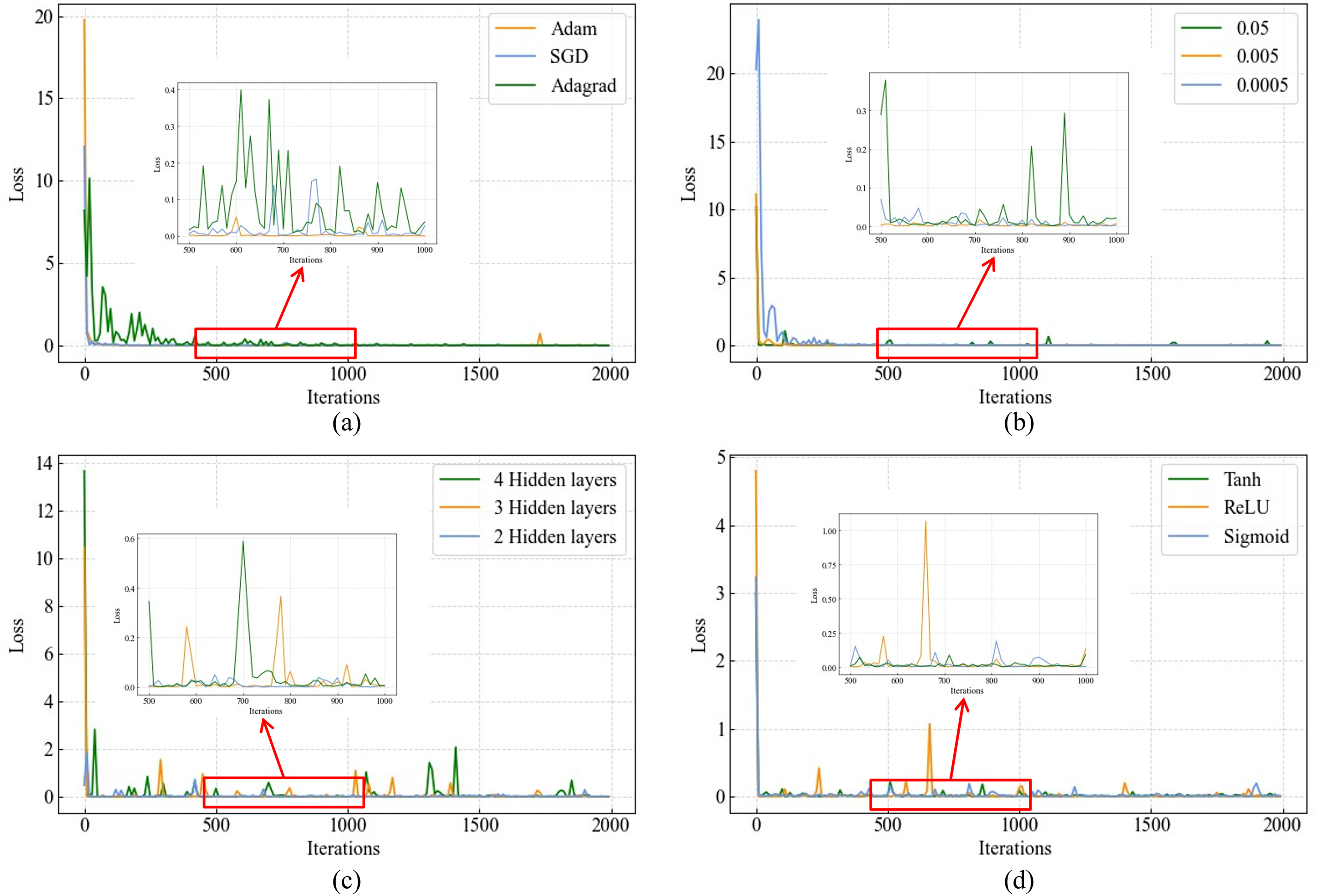
Figure 5: Training loss variation under different hyperparameter settings: (a) Optimizer; (b) Learning rate; (c) Number of hidden layers; (d) Activation function

Additionally, the effects of dropout and weight decay were considered, as shown in the Fig. 6.

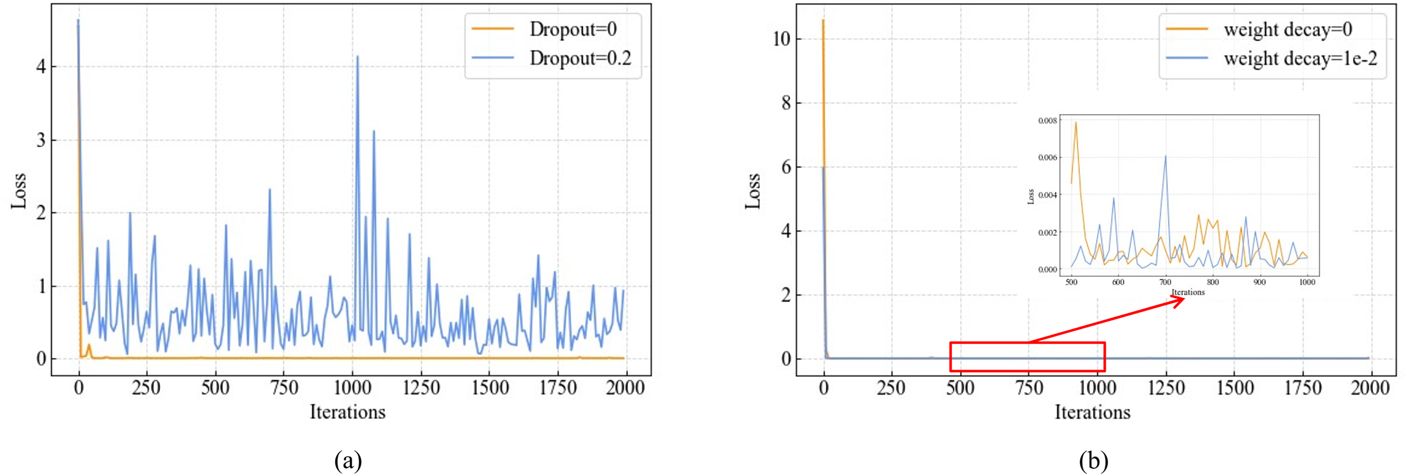
Figure 6: Training loss variation under different hyperparameter settings: (a) Dropout; (b) Weight decay

When dropout is applied, the loss increases because the dataset is small and does not require an overly complex network structure, so dropout can be omitted. Regarding weight decay, the loss curves for both training and test sets are essentially identical with minimal differences, so weight decay was not employed in this study.

Upon completion of training, the DNN model can accurately and efficiently predict sound pressure responses under varying uncertain conditions. This surrogate model significantly accelerates uncertainty analysis, particularly in scenarios where conventional Monte Carlo simulations are computationally infeasible. In the next section, a case study on a spherical model is presented to validate the accuracy and effectiveness of the proposed DNN-based framework.

5  Numerical Examples

In this section, we present a series of numerical experiments to evaluate the effectiveness and accuracy of the proposed isogeometric BEM approach combined with a deep neural network (DNN) surrogate model for uncertainty quantification in acoustic problems. The acoustic BEM solver was developed in Fortran 90 using Catmull-Clark subdivision surfaces, while the DNN model was implemented in Python using PyTorch. All simulations assume the material properties of structural steel. A flowchart outlining the computational pipeline is shown in Fig. 7.

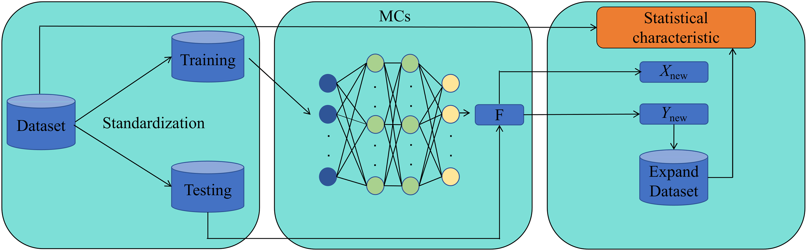
Figure 7: Flow of DNN-based uncertainty analysis

5.1 Spherical Model

To validate the proposed isogeometric BEM framework, we examine a classical acoustic scattering problem: a rigid sphere with a radius of 5 m subjected to a unit-amplitude plane wave propagating along the x-axis. This configuration serves as a widely recognized benchmark in three-dimensional acoustics due to its well-established analytical solution, providing a reliable reference for assessing numerical accuracy and convergence properties.

The BEM model is constructed using Catmull-Clark subdivision surfaces to generate a smooth geometric representation from an initial coarse polygonal mesh. The refined mesh and simulation setup are illustrated in Fig. 8.

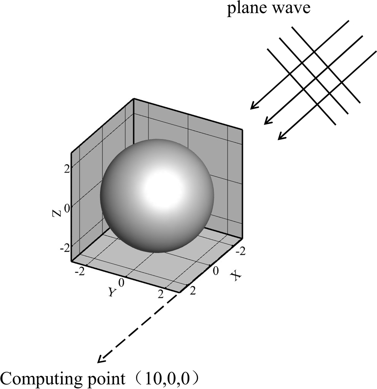
Figure 8: Problem setup for the spherical model: incident wave and mesh

The Catmull-Clark refinement process is visualized in Fig. 9, where the control mesh is iteratively smoothed into a limit surface. This approach enables the generation of analysis-suitable geometry with C1 continuity, which is particularly advantageous in acoustic problems involving curvature-sensitive wave propagation.

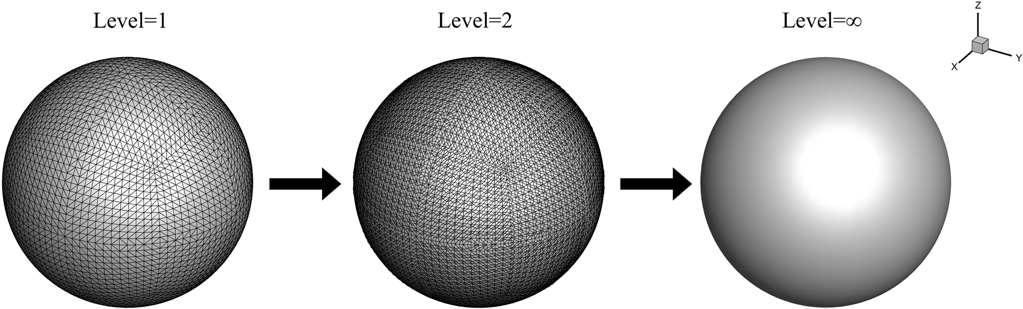
Figure 9: Subdivision refinement of the sphere using Catmull-Clark surfaces

To assess accuracy, the complex-valued sound pressure field (both real and imaginary parts) is computed across a frequency range of 20–200 Hz and compared against the analytical Mie solution. As shown in Fig. 10, the BEM results match the analytical solution with high fidelity, validating the geometric and numerical consistency of the implementation. The sound pressure gradually increases with frequency. However, this accuracy comes at a computational cost: as mesh resolution increases, the number of degrees of freedom and the size of dense BEM system matrices grow substantially, leading to increased memory requirements and longer simulation times.

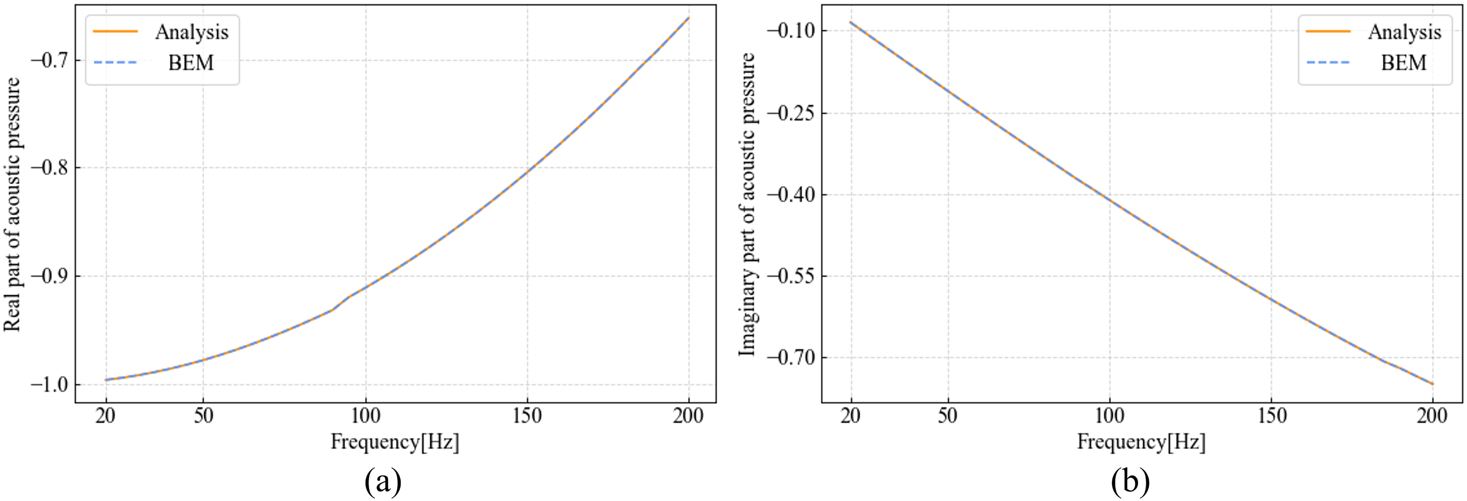
Figure 10: Comparison of BEM results with analytical solution: (a) Real part; (b) Imaginary part

To overcome this bottleneck, we leverage a DNN-based surrogate model—trained on a subset of BEM solutions as described in Section 4—to enable fast and accurate prediction of acoustic responses under parametric uncertainty. This surrogate model drastically reduces the need for repeated full-scale BEM evaluations, offering a scalable solution for uncertainty quantification while maintaining high prediction accuracy.

Subsequently, we evaluated a point on the sphere surface and computed the responses at different frequencies using both the BEM and the DNN models, comparing them with the analytical solution. This further verifies the accuracy of both BEM and DNN.

As shown in the Fig. 11, even when there are significant discrepancies between the BEM and the analytical solution on the sphere surface, the DNN predictions still align well with the BEM results. This is because the DNN learns patterns directly from the data.

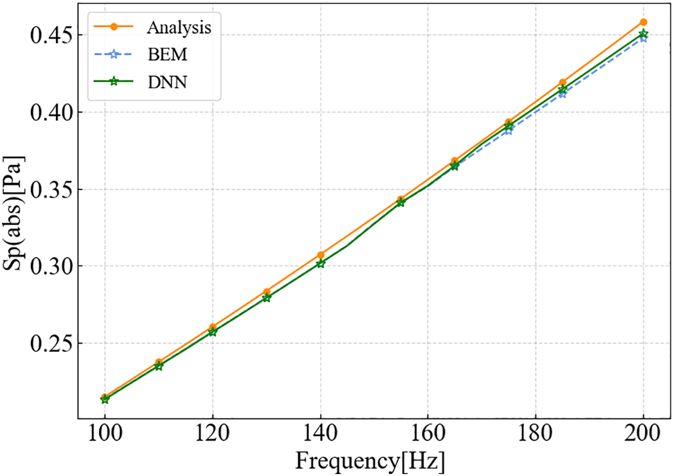
Figure 11: Comparison of BEM and DNN results with analytical solution

To demonstrate the capability of the proposed DNN surrogate model, we investigate the influence of three key physical parameters on the sound pressure response: the absorption coefficient of the acoustic material, the ground reflection coefficient, and the vertical distance between the sphere’s center and the ground plane. These parameters were chosen due to their practical relevance and inherent variability in real-world acoustic environments. The analysis is conducted at two representative frequencies—100 and 200 Hz—to capture the frequency-dependent behavior of acoustic interactions.

To assess the predictive accuracy of the DNN, we compare its output against full-order BEM simulations. The DNN is trained using data sampled at a coarse interval of 10 units, and its predictive generalization is evaluated by applying it to a finer test set sampled at unit intervals. The comparison results for the one-dimensional input case are presented in Fig. 12.

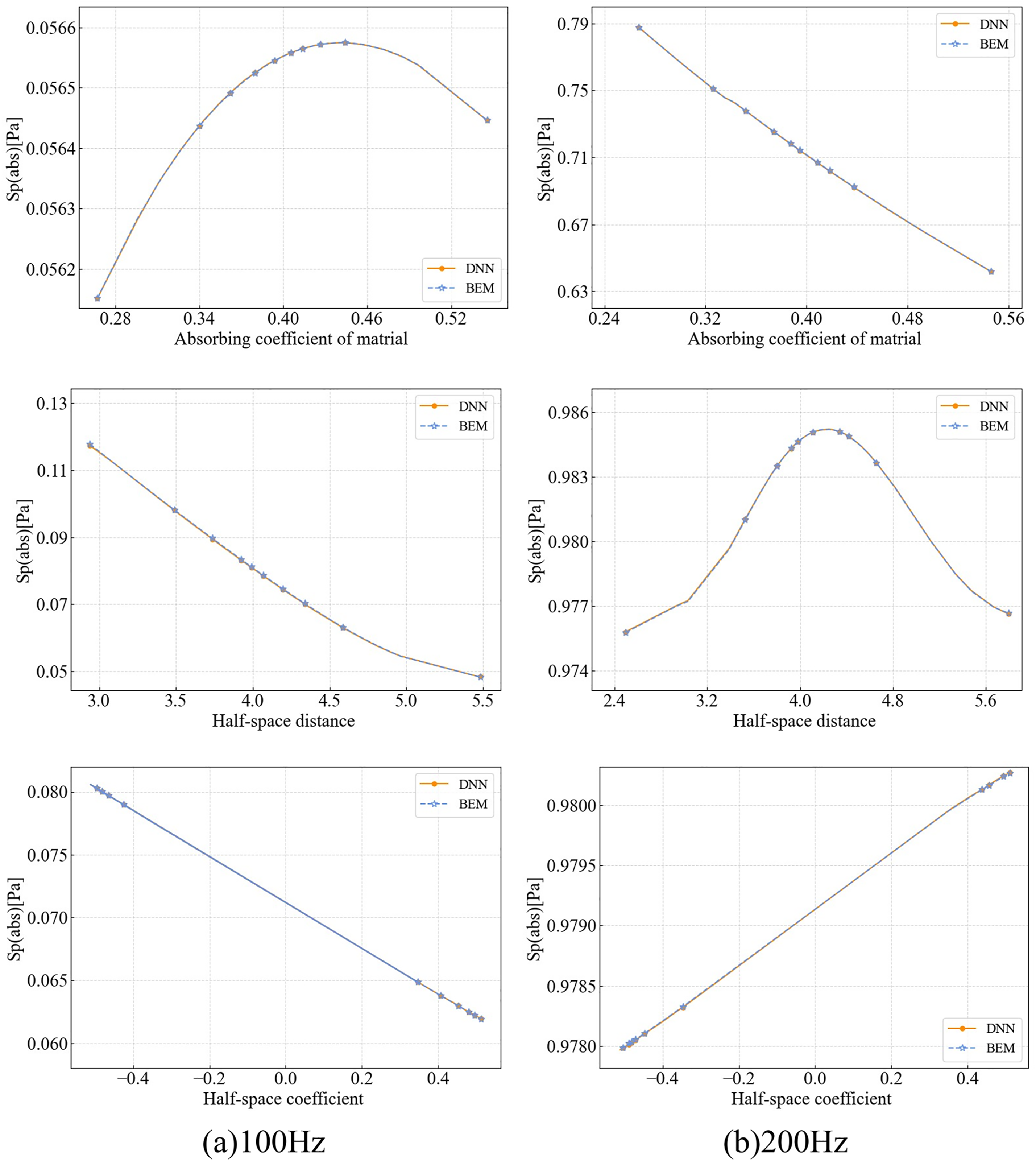
Figure 12: Comparison between DNN and BEM: (a) 100 Hz; (b) 200 Hz

As shown in Fig. 12, the DNN predictions exhibit excellent agreement with the full-order BEM results across all parametric scenarios. The model accurately captures both monotonic and non-monotonic response trends, demonstrating strong generalization capability and learning robustness. These results indicate that the DNN surrogate has successfully learned the underlying input–output mapping, rather than simply interpolating between training samples.

From a physical standpoint, the parametric trends reveal insightful acoustic behavior:

•   Absorption Coefficient: At 100 Hz, increasing the absorption coefficient initially causes an increase in sound pressure, followed by a reduction. This non-monotonic behavior is attributed to a resonance-like effect where partial absorption alters the interference between direct and reflected waves. At 200 Hz, a higher absorption coefficient leads to a monotonic decrease in sound pressure, reflecting the enhanced damping capacity of the material at higher frequencies due to reduced wavelength.

•   Sphere-to-Ground Distance: At lower frequencies, sound pressure increases approximately linearly with distance, which is consistent with classical ground effect theory for long wavelengths. At 200 Hz, however, the trend becomes nonlinear, showing a peak followed by attenuation. This indicates stronger interference effects arising from phase differences between direct and ground-reflected waves, especially at higher frequencies.

•   Ground Reflection Coefficient: Interestingly, the effect of this parameter reverses with frequency. At 100 Hz, increasing the reflection coefficient raises the observed sound pressure, while at 200 Hz, it leads to a suppression. This frequency-dependent behavior is governed by the interaction between reflected and incident waves, which is highly sensitive to phase shifts and propagation paths.

To evaluate the scalability and robustness of the DNN surrogate model, we further test it under higher-dimensional input scenarios. Fig. 13 presents results for cases where two parameters vary simultaneously, while Fig. 14 illustrates predictions across the full three-variable input space.

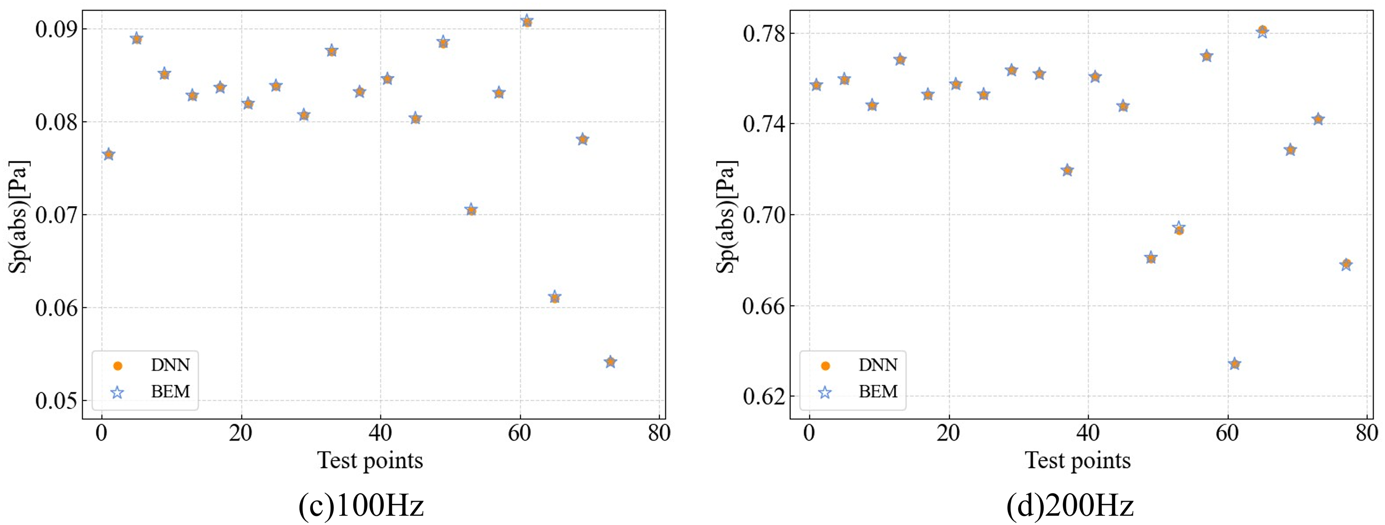
Figure 13: Comparison of sound pressure predictions from the BEM and DNN surrogate model under two-variable input variations at 100 and 200 Hz. (a), (b): Variations with absorption coefficient and ground reflection coefficient. (c), (d): Variations with absorption coefficient and sphere-to-ground distance

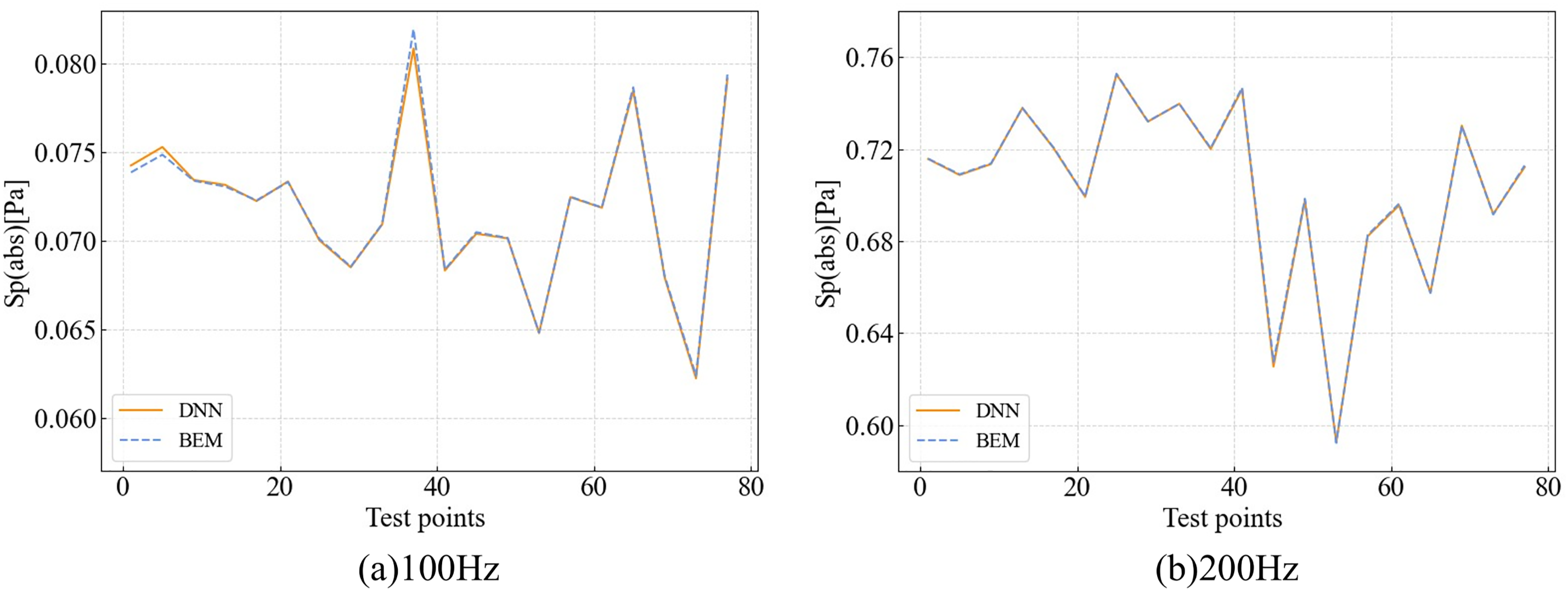
Figure 14: Comparison of BEM and DNN sound pressure predictions under simultaneous variation of all three input parameters (absorption coefficient, ground reflection coefficient, and sphere-to-ground distance). (a): Results at 100 Hz; (b): Results at 200 Hz

Fig. 13 shows variations in sound pressure at 100 and 200 Hz under two-parameter changes. The first row examines the combined effects of the absorption coefficient and the ground reflection coefficient, while the second row considers the absorption coefficient and the vertical distance to the ground. In all cases, DNN predictions exhibit excellent agreement with full-order BEM simulations. The surrogate model accurately captures both smooth trends and more complex interactions arising from coupled parameter changes, demonstrating strong generalization ability and stability in multi-variable acoustic scenarios. Fig. 14 compares DNN and BEM predictions for the full three-variable configuration. Despite the increased complexity in the pressure response, the DNN model retains high accuracy, with prediction error—measured via mean absolute percentage error (MAPE)—remaining below 2%. The close correspondence across the full test space confirms the model’s robustness and its suitability for efficient uncertainty propagation in high-dimensional parameter spaces.

The statistical performance of the DNN surrogate model under varying input dimensions and frequencies is summarized in Table 3. Two key evaluation metrics are reported: the mean absolute percentage error (MAPE) and the coefficient of determination (R2).

In general, a lower MAPE indicates smaller prediction error, with values below 5% typically considered highly accurate. Similarly, R2 values close to 1 reflect an excellent model fit. As shown in Table 3, the DNN model maintains strong predictive performance across different input dimensions and frequencies. Most MAPE values remain well below 0.05, and all R2 values exceed 0.98, demonstrating the surrogate model’s capability to effectively approximate full-order BEM solutions. However, as the input dimensionality increases from 1D to 3D, there is a slight degradation in accuracy, as evidenced by higher MAPE values and minor reductions in R2. This trend reflects the increased complexity of learning in higher-dimensional input spaces, where capturing intricate interactions between multiple parameters presents a greater challenge to surrogate modeling.

To further investigate the spatial behavior of acoustic responses, Fig. 15 presents the surface sound pressure distribution on the spherical model under varying absorption coefficients. In subplot (a), the sphere remains 5 m above the ground with a fixed material absorption coefficient of 0.1, while the ground reflection coefficient is varied. The resulting pressure distributions show minimal variation, indicating that surface sound pressure on the sphere is relatively insensitive to ground reflection when the object is sufficiently elevated. In contrast, subplot (b) analyzes changes in the vertical position of the sphere above the ground. Here, the ground reflection coefficient and absorption coefficient are fixed at 0.4 and 0.1, respectively. The results reveal that increasing the height significantly alters the surface pressure distribution, indicating stronger interference effects and path-length sensitivity. These spatial patterns are consistent with the trends observed at specific monitoring points and confirm the physical reliability of the simulation results.

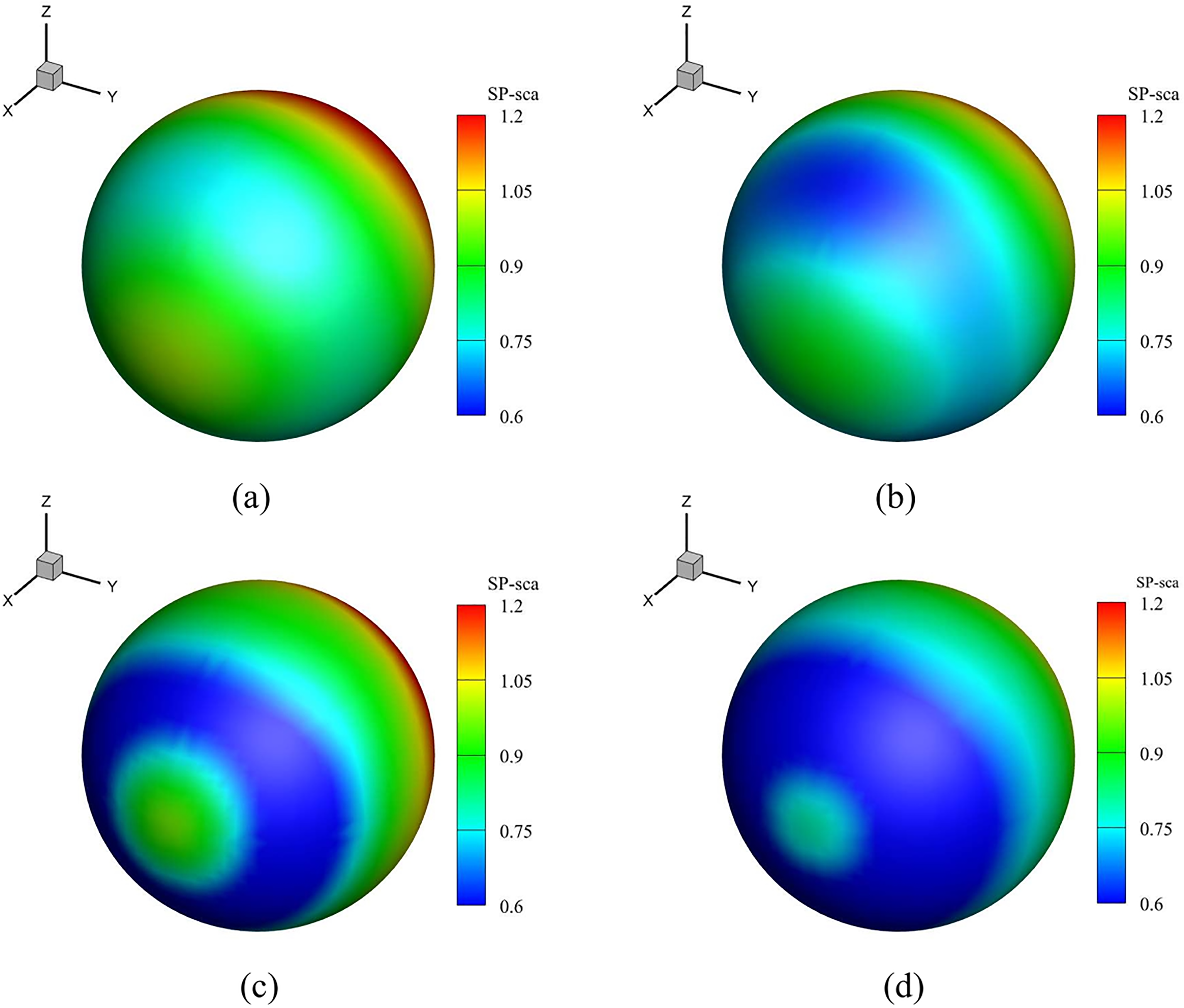
Figure 15: Surface sound pressure distributions on the sphere under different absorption conditions. (a), (b): Frequency = 100 Hz; absorption coefficient = 0.3 and 0.6, respectively. (c), (d): Frequency = 200 Hz; absorption coefficient = 0.3 and 0.6, respectively

Fig. 16 further explores how the ground reflection coefficient and sphere-to-ground distance affect the surface sound pressure distribution. When analyzing the effect of the ground reflection coefficient, the model is positioned 5 m above the ground with the absorption coefficient fixed at 0.1. Conversely, to evaluate the influence of height, the ground reflection coefficient and absorption coefficient are set to 0.4 and 0.1, respectively. The results show that variations in the ground reflection coefficient have minimal impact on the surface sound pressure, a trend that aligns with earlier observations at the monitoring point. In contrast, changes in the height above the ground, particularly from 2 to 5 m, result in more pronounced variations, indicating that vertical positioning has a greater influence on the acoustic response.

Figure 16: Effect of environmental parameters on sound pressure distribution over the sphere surface. (a): Ground reflection coefficients = 0.2, 0.5, 0.8 (fixed height = 5 m, absorption coefficient = 0.1). (b): Sphere-to-ground distances = 2, 5, 8 m (fixed ground reflection coefficient = 0.4, absorption coefficient = 0.1)

To further validate the effectiveness of the DNN surrogate model, the statistical moments, namely the expectation and standard deviation, of the predicted sound pressure values using DNN are compared against those obtained from the BEM simulations. Table 4 presents this comparison across different input dimensions and frequencies. It demonstrates that the DNN model accurately captures both the mean and variability of the sound pressure predicted by the BEM method across all tested scenarios. In the 1-D cases, where individual parameters such as the absorption coefficient, ground reflection coefficient, or height are varied independently, the DNN predictions are nearly identical to those of the full BEM simulation, confirming the surrogate’s strong approximation capability in low-dimensional settings.

In the 2-D case—where the absorption coefficient and height are varied simultaneously—the DNN continues to deliver highly accurate predictions, with negligible deviations in both mean and standard deviation. In the 3-D scenario, despite the increase in nonlinearity and interaction complexity due to simultaneous variation of all parameters, the DNN maintains a satisfactory performance. The prediction errors remain within acceptable limits, validating the surrogate model’s potential for accelerating uncertainty quantification in high-dimensional acoustic simulations.

Moreover, the small differences in the mean values suggest that the average effect of the varying parameters on sound pressure remains relatively stable. However, the standard deviations reveal significant differences in uncertainty contribution: the material absorption coefficient contributes the most to variability in sound pressure, while the ground reflection coefficient has a minimal impact. As the dimensionality of the input increases, the standard deviation generally rises as well, indicating that the interaction of multiple uncertain parameters enhances the overall uncertainty in the system. These observations highlight the importance of carefully analyzing the role of absorbing materials in acoustic uncertainty studies.

5.2 Washing Model

In this section, a washing machine model with a complex geometric structure is investigated to evaluate the effectiveness of a deep neural network (DNN) in accelerating uncertainty analysis. The model is subjected to a unit-amplitude plane wave incident along the x-axis, with a wave number of 0.100. The acoustic response is observed at a point located 1 m from the source, as illustrated in Fig. 17.

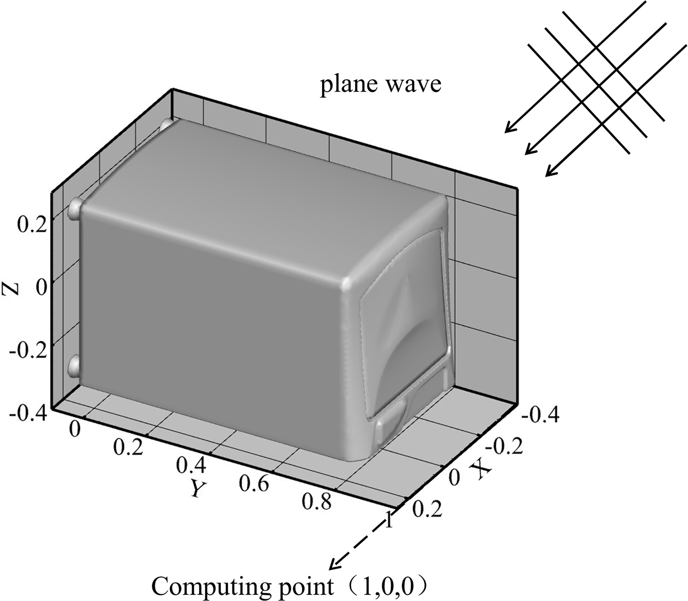
Figure 17: Acoustic scattering of a washing model

The washing machine model consists of 21,818 boundary elements and 10,920 nodes. Similar to previous cases, we analyze how variations in material and environmental parameters influence the acoustic response. The comparisons between DNN predictions and BEM results are shown in Fig. 18 for one-dimensional parameter changes and in Fig. 19 for higher-dimensional inputs. The results show that the DNN achieves accuracy comparable to that of the BEM solver across all cases. Slight fluctuations are observed at the boundaries of plots (a) and (b) in Fig. 18, attributed to the relatively sparse training data in those regions. These can be mitigated by selectively increasing the number of training samples near the edges. Nevertheless, the overall error remains below 2%, underscoring the high fidelity of the DNN predictions.

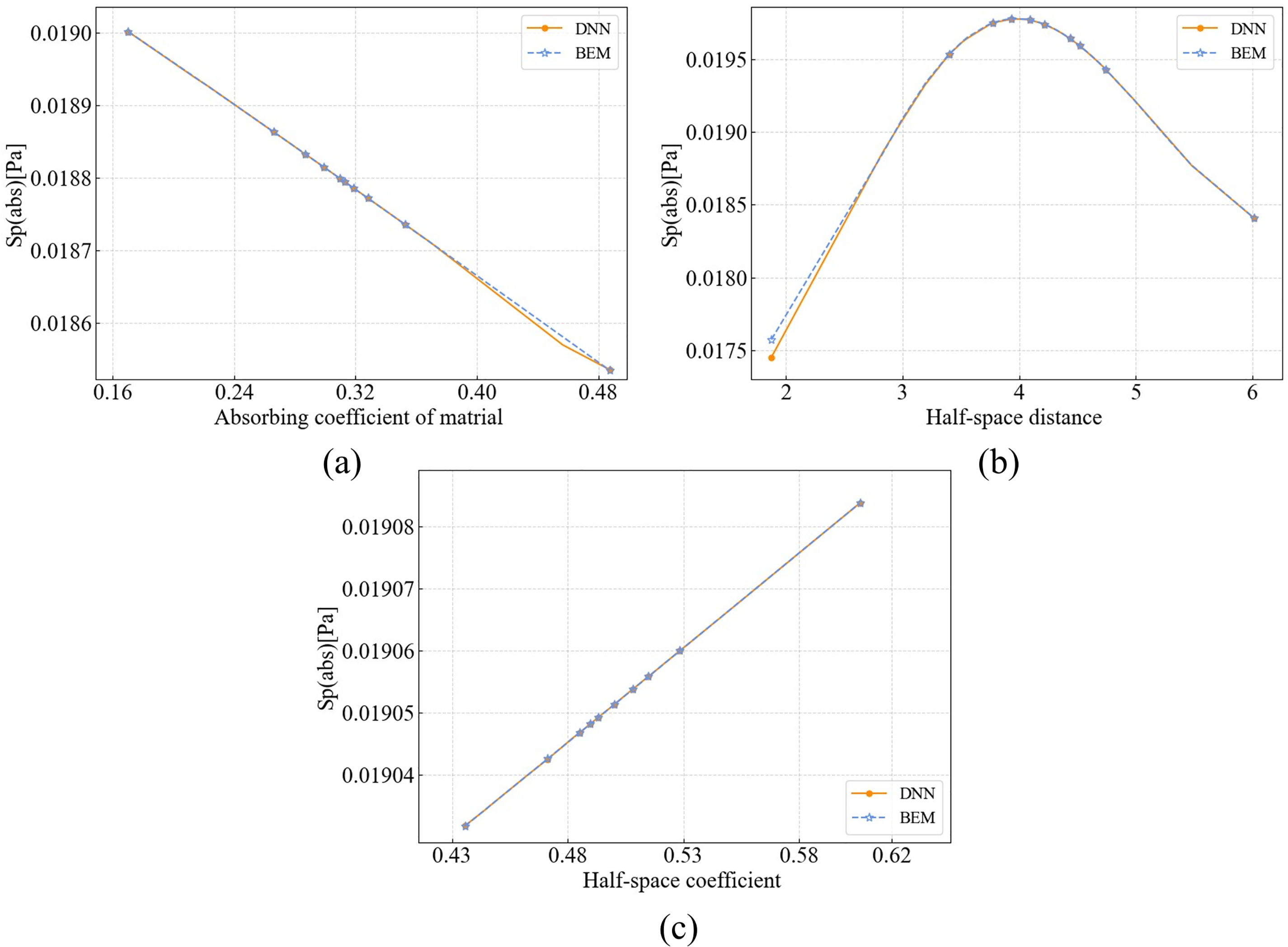
Figure 18: Comparison between DNN and BEM at 150 Hz under single-parameter variations: (a) Absorption coefficient; (b) Sphere-to-ground distance; (c) Ground reflection coefficient

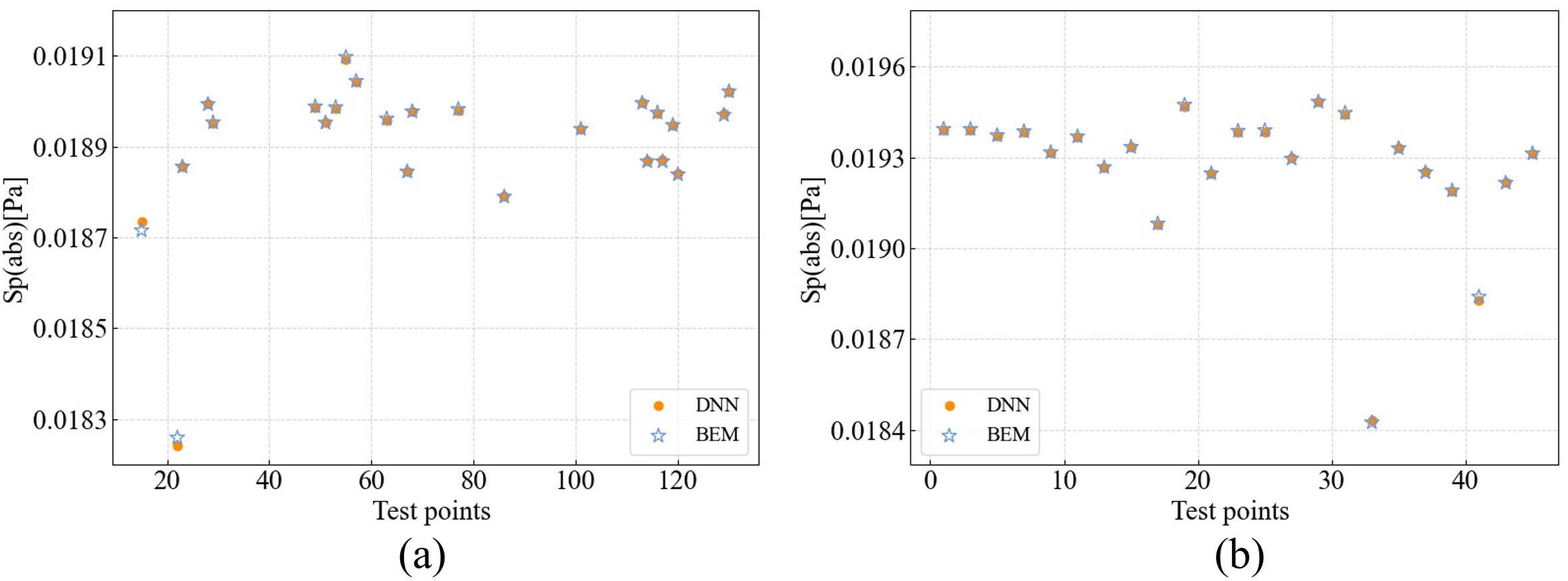
Figure 19: Comparison between DNN and BEM at 150 Hz under multi-parameter variations: (a) Absorption coefficient and ground distance; (b) All three parameters

To further explore environmental effects, we calculate surface sound pressure contours at varying frequencies and model heights, as presented in Fig. 20. It is evident that increasing the frequency leads to pronounced changes in the sound pressure distribution. Along the z-axis of the model, the surface sound pressure generally decreases with frequency, whereas in other regions, the pressure may increase. Changing the height from 1 to 3 m results in only slight numerical differences, while the overall distribution pattern remains largely unchanged.

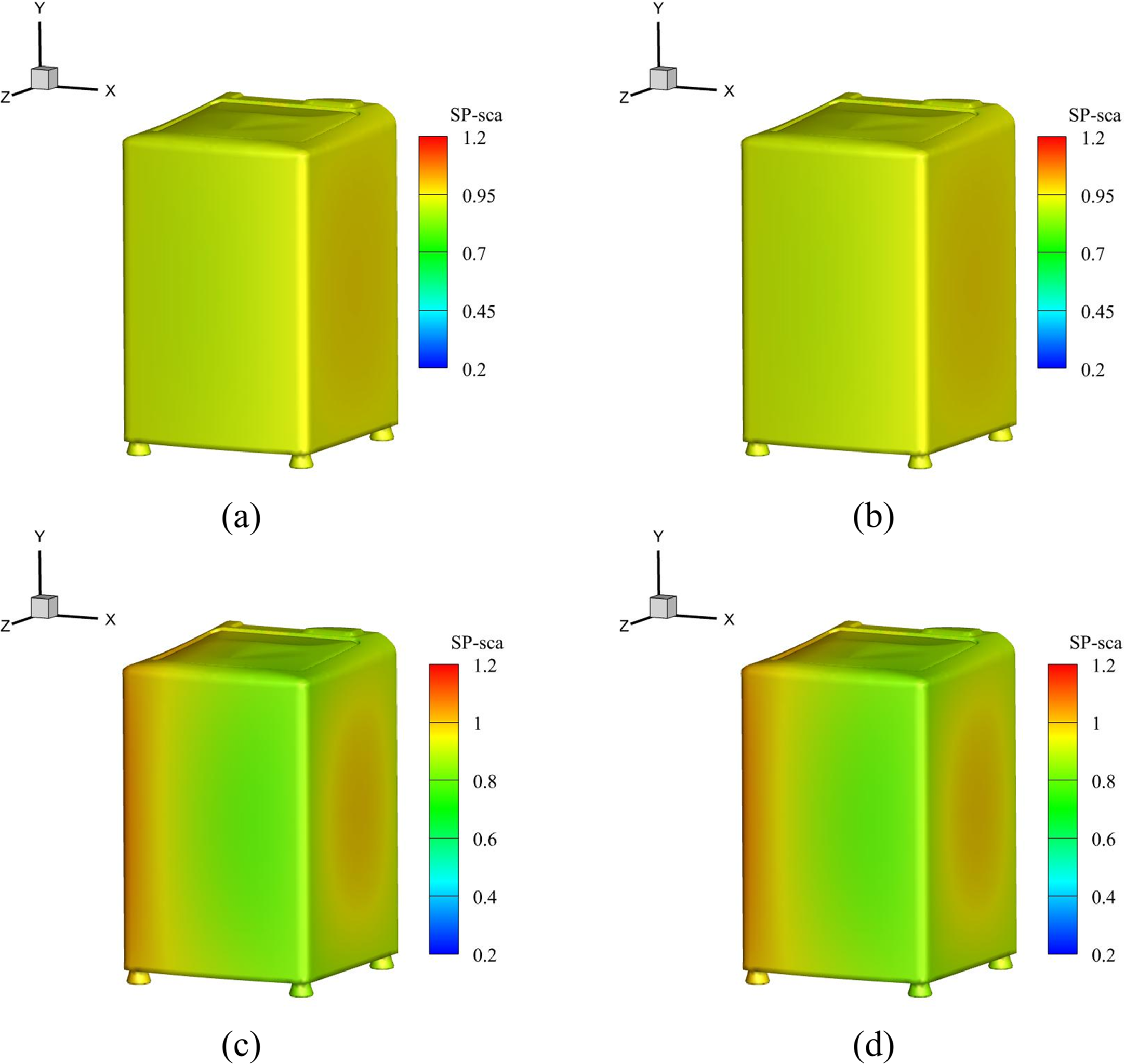
Figure 20: Surface sound pressure contours of the washing machine: (a) 200 Hz, half-space distance = 1 m; (b) 200 Hz, half-space distance = 3 m; (c) 400 Hz, half-space distance = 1 m; (d) 400 Hz, half-space distance = 3 m

These findings suggest that the DNN’s predictive capability is not hindered by the geometric complexity or mesh density of the model. Since the DNN learns data patterns directly from the training samples, it remains robust even when applied to intricate geometries. In this study, computing 160 data samples with BEM alone required 30,241.87 s. In contrast, the DNN-accelerated BEM approach only required computing data points at interval of 10 for training, followed by predictions at an interval of 1.

The time required for generating the training dataset was 2946.29 s. The training time for the corresponding DNN model is approximately 30 min, and inference for the entire dataset required just 1.87 s. Therefore, the time consumed by the DNN model is less than that of the standalone BEM method. These results highlight the significant computational savings and practical advantages offered by the DNN-accelerated BEM approach in large-scale acoustic simulations.

To quantitatively assess the accuracy and robustness of the DNN surrogate model, we compare statistical measures of the predicted sound pressure against the benchmark BEM results. The evaluation focuses on three types of input dimensionalities: one-dimensional (1-D), two-dimensional (2-D), and three-dimensional (3-D), all at a frequency of 150 Hz. The input parameters include the absorption coefficient of the material, the half-space distance, and the half-space reflection coefficient. Table 5 summarizes the expectation and standard deviation for both methods under these conditions.

Finally, we summarized the data from the sphere and washing machine cases, expressing the influence of each parameter on the sound pressure using Eq. (32). The results are presented in the Table 6.

ΔX=max(Xi)−min(Xi),i=1,2,…,nΔP=Xmax(Pi)−min(Pi),i=1,2,…,nS=|ΔPΔX⋅X¯P¯|(32)

Here, X¯ and Y¯ denote the mean values. We found that the distance from the ground has the most significant impact on the sound pressure, playing a dominant role, followed by the absorption material.

5.3 Coffee Machine Model

In this section, a more geometrically intricate model—a coffee machine—is employed to investigate the impact of complex geometry on BEM calculations, as well as to evaluate the effectiveness of DNN-based acceleration. The model is subjected to a unit-amplitude plane wave incident along the x-axis, with a wave number of 0.100. The acoustic response is observed at a point located 0.25 meters from the source, as shown in Fig. 21. The coffee machine model consists of 7890 nodes and 15,776 elements.

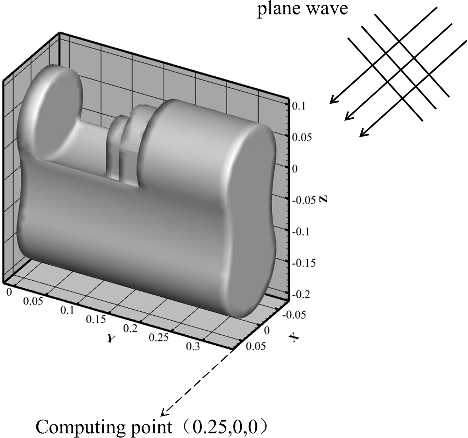
Figure 21: Acoustic scattering of a washing model

Using the same methodology as in the previous section, the sound pressure is computed with both BEM and DNN approaches. The expectation and standard deviation are then evaluated to analyze statistical behavior under uncertainty. The detailed results are shown in Fig. 22.

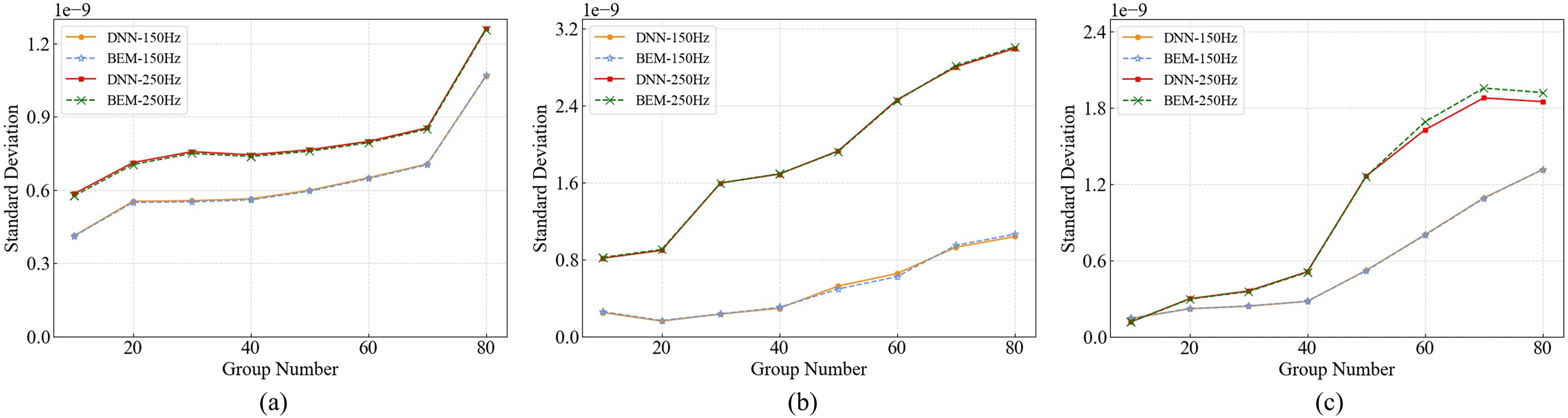
Figure 22: Comparison of standard deviation between BEM and DNN at various frequencies: (a) 1-D input (absorption coefficient); (b) 2-D input (absorption coefficient and half-space distance); (c) 3-D input (all parameters)

Fig. 22a–c illustrates the trends of the sound pressure standard deviation obtained at 150 and 250 Hz as the amount of Monte Carlo data increases. In all cases, both DNN and BEM show an increasing trend with the number of samples, reflecting that the uncertainty in the simulation results grows as the sample size expands. For one-dimensional and two-dimensional inputs, the DNN results are highly consistent with BEM, exhibiting the same trend, while slight deviations appear in the three-dimensional case, which is attributed to the increased complexity of the input parameters. Nevertheless, the overall discrepancy remains small. In addition, the DNN demonstrates higher stability at lower frequencies, whereas more pronounced fluctuations are observed at higher frequencies, particularly at 250 Hz. This indicates that the acoustic response becomes more sensitive to geometric and parametric variations as frequency increases.

To further explore spatial acoustic behavior, Fig. 23 presents sound pressure contour plots on the coffee machine surface at four different frequencies.

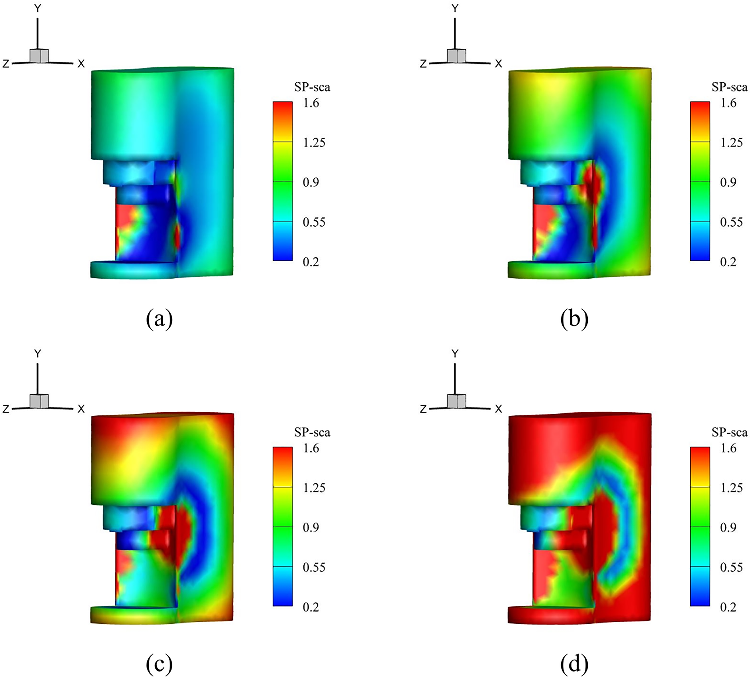
Figure 23: Surface sound pressure contours of the coffee machine at different frequencies: (a) 100 Hz; (b) 150 Hz; (c) 200 Hz; (d) 250 Hz

As shown in Fig. 23, sound pressure distributions vary significantly across frequencies. Regions with complex geometrical features consistently exhibit higher sound pressure levels, particularly in the range of 200–250 Hz. These results highlight the importance of geometry-induced effects in acoustic scattering, and further confirm the capability of DNN to accurately approximate BEM responses even for geometrically complex models.

6  Conclusion

This study proposes a method to improve the sampling efficiency of the Monte Carlo (MC) method and reduce the computational cost associated with traditional boundary element method (BEM) simulations. By leveraging deep neural networks (DNNs) as surrogate models, high-fidelity acoustic data can be rapidly generated after training on a relatively small dataset. To further enhance numerical accuracy, the Catmull-Clark subdivision surface technique is employed to construct high-quality meshes, ensuring geometric fidelity and solution precision.

Validation cases demonstrate that DNN-predicted sound pressure levels closely match those obtained from conventional BEM computations. The introduction of DNN-based acceleration yields a substantial reduction in overall computation time, confirming the effectiveness of this approach for uncertainty quantification. Moreover, Monte Carlo analyses reveal that statistical properties—such as expectation and standard deviation—of DNN-generated samples align closely with those from BEM, even under increasing input dimensionality.

Importantly, when applied to models with complex geometries and high mesh densities, the DNN maintains both accuracy and robustness. These findings underscore the broad applicability and potential of the proposed DNN-accelerated framework for efficient and scalable acoustic analysis in engineering contexts.

Compared with traditional ANN models, the DNN model demonstrates higher robustness and better predictive performance, while its training is less demanding than generative neural networks such as GANs. However, the proposed method also has limitations. If the underlying model has a coarse mesh, resulting in lower-quality computational data, the DNN’s predictions may be adversely affected, leading to reduced accuracy and longer training times. Additionally, the computational model simplifies certain geometric features, whereas real-world models may be more complex. Some assumptions are also made regarding the physical problem; for instance, acoustic–structural coupling effects are not considered. In future work, we will explore different neural network approaches to achieve faster and more accurate stochastic analysis.

Acknowledgement: The authors would like to express their sincere thanks to Dr. Leilei Chen from Huanghuai University for his valuable suggestions in improving this manuscript.

Funding Statement: The authors are grateful for the financial support provided by the Postgraduate Education Reform and Quality Improvement Project of Henan Province (Grant Nos. YJS2023JD52 and YJS2025GZZ48). The Zhumadian 2023 Major Science and Technology Special Project (Grant No. ZMD SZDZX2023002). The Zhumadian 2024 Major Science and Technology Special Project (Grant No. ZMDSZDYF2024007). 2025 Henan Province International Science and Technology Cooperation Project (Cultivation Project, No. 252102521011). Research Merit-Based Funding Program for Overseas Educated Personnel in Henan Province (Letter of Henan Human Resources and Social Security Office [2025] No. 37).

Author Contributions: The authors confirm contribution to the paper as follows: study conception and design: Yingying Guo, Pei Li; data collection: Yingying Guo, Ziyu Cui; analysis and interpretation of results: Yingying Guo, Ziyu Cui, Pei Li; draft manuscript preparation: Ziyu Cui, Jibing Shen; manuscript revision: Pei Li. All authors reviewed the results and approved the final version of the manuscript.

Availability of Data and Materials: The datasets generated or analyzed during the current study are available from the corresponding author on reasonable request.

Ethics Approval: Not applicable.

Conflicts of Interest: The authors declare no conflicts of interest to report regarding the present study.

Appendix A Evaluation of Singular Integrals

When the source point approaches the field point, i.e., the distance r between them tends to zero, the fundamental solution kernel G=eik¯r4πr becomes weakly singular. Conventional Gauss quadrature is inadequate for accurately evaluating such integrals. To address this, we employ a polar coordinate transformation to efficiently handle weakly singular integrals over three-dimensional surface elements, using 10 Gauss quadrature points for both regular and singular integrands.

The origin of the polar coordinate system is placed at the source point x, with local coordinates (ξs,ηs). The transformation from local to polar coordinates is given by:

ξ=ξs+ρ¯cosθ,η=ηs+ρ¯sinθ.

By subdividing the original triangular element based on the position of the source point within the element, the integral of the kernel function G in Eq. (18) is rewritten as:

∑k=1Nv∑l=1Nm∫θl−1θl∫0r^G(ρ¯,θ)N^ℓ(ξ,η)(ρ¯,θ)|J(ρ¯,θ)|ρ¯d⁡ρ¯d⁡θpkE,(A1)

where Nm is the number of polar sub-elements, (θl−1,θl) defines the angular boundaries of each sub-element, r^=he/cos⁡θ¯, and E denotes the element containing the source point x.

After transformation, the integrals become regular. In fact, the double-layer kernel in Eq. (18) is only weakly singular near the source point, since ∂G∂n depends on ∂r∂n. Thus, using the polar coordinate transformation, the integrals involving ∂G∂n can be evaluated both efficiently and accurately.

Appendix B Hyper-Singular Integrals

To address hyper-singular integrals, the regularization technique is employed by subtracting and adding the normal derivative of the static Green’s function G¯, where ∂G¯∂n=14πr2. This yields:

∫Γ∂2G(x,y)∂n(y)∂n(x)p(y)d⁡Γ=∫Γ[∂2G(x,y)∂n(y)∂n(x)−∂2G¯(x,y)∂n(y)∂n(x)]p(y)d⁡Γ+∫Γ∂2G¯(x,y)∂n(y)∂n(x)p(y)d⁡Γ.(A2)

The first term on the right hand side in the above equation is non-singular and the second term can be expanded using Taylor series:

∫Γ∂2G¯(x,y)∂n(y)∂n(x)p(y)d⁡Γ(y)=∫Γ∂2G¯(x,y)∂n(y)∂n(x)[p(y)−p(x)−∇p(x)(y−x)]d⁡Γ(y)+p(x)∫Γ∂2G¯(x,y)∂n(y)∂n(x)d⁡Γ(y)+∇p(x)∫Γ∂2G¯(x,y)∂n(y)∂n(x)(y−x)d⁡Γ(y)(A3)

where ∇p(x)=∂p(x)∂v1v1+∂p(x)∂v2v2 and v1,v2 are two tangent vectors at point x on the surface.

The last two integrals in Eq. (A3) can be evaluated analytically:

∫Γ∂2G¯(x,y)∂n(y)∂n(x)d⁡Γ=0,(A4)

∫Γ∂2G¯(x,y)∂n(y)∂n(x)(y−x)d⁡Γ=∫Γ∂G¯(x,y)∂n(x)n(y)d⁡Γ−12n(x).(A5)

Substituting Eqs. (A4) and (A5) into Eq. (A3) yields:

∫Γ∂2G¯(x,y)∂n(y)∂n(x)p(y)d⁡Γ=∫Γ∂2G¯(x,y)∂n(y)∂n(x)[p(y)−p(x)−(∂p(x)∂v1v1+∂p(x)∂v2v2)(y−x)]d⁡Γ+∂p(x)∂v1∫Γ∂G¯(x,y)∂n(x)v1⋅n(y)d⁡Γ−12∂p(x)∂v1v1⋅n(x)+∂p(x)∂v2∫Γ∂G¯(x,y)∂n(x)v2⋅n(y)d⁡Γ−12∂p(x)∂v2v2⋅n(x)(A6)

Finally, substituting Eq. (A6) into Eq. (A2), the original hyper-singular integral is expressed as:

∫Γ∂2G(x,y)∂n(y)∂n(x)p(y)d⁡Γ=∫Γ[∂2G(x,y)∂n(y)∂n(x)−∂2G¯(x,y)∂n(y)∂n(x)]p(y)d⁡Γ+∫Γ∂2G¯(x,y)∂n(y)∂n(x)[p(y)−p(x)−(∂p(x)∂v1v1+∂p(x)∂v2v2)(y−x)]d⁡Γ+∂p(x)∂v1∫Γ∂G¯(x,y)∂n(x)v1⋅n(y)d⁡Γ−12∂p(x)∂v1v1⋅n(x)+∂p(x)∂v2∫Γ∂G¯(x,y)∂n(x)v2⋅n(y)d⁡Γ−12∂p(x)∂v2v2⋅n(x)(A7)

References

1. Zhao H, Fu C, Zhang Y, Zhu W, Lu K, Francis EM. Dimensional decomposition-aided metamodels for uncertainty quantification and optimization in engineering: a review. Comput Methods Appl Mech Eng. 2024;428:117098. doi:10.1016/j.cma.2024.117098. [Google Scholar] [CrossRef]

2. Chen L, Lian H, Xu Y, Li S, Liu Z, Atroshchenko E, et al. Generalized isogeometric boundary element method for uncertainty analysis of time-harmonic wave propagation in infinite domains. Appl Mathem Model. 2023;114(39–41):360–78. doi:10.1016/j.apm.2022.09.030. [Google Scholar] [CrossRef]

3. Zou Z, Meng X, Karniadakis GE. Uncertainty quantification for noisy inputs-outputs in physics-informed neural networks and neural operators. Comput Methods Appl Mech Eng. 2025;433(6):117479. doi:10.1016/j.cma.2024.117479. [Google Scholar] [CrossRef]

4. Chen LL, Huo RJ, Lian H, Yu B, Zhang MX, Natarajan S, et al. Uncertainty quantification of 3D acoustic shape sensitivities with generalized nth-order perturbation boundary element methods. Comput Methods Appl Mech Eng. 2025;433(4):117464. doi:10.1016/j.cma.2024.117464. [Google Scholar] [CrossRef]

5. Wang C, Hong L, Qiang X, Xu M. Novel numerical method for uncertainty analysis of coupled vibro-acoustic problem considering thermal stress. Comput Methods Appl Mech Eng. 2024;420:116727. doi:10.1016/j.cma.2023.116727. [Google Scholar] [CrossRef]

6. Hamdia KM, Ghasemi H, Zhuang X, Rabczuk T. Multilevel Monte Carlo method for topology optimization of flexoelectric composites with uncertain material properties. Eng Anal Bound Elem. 2022;134(13):412–8. doi:10.1016/j.enganabound.2021.10.008. [Google Scholar] [CrossRef]

7. Baumgarten N, Krumscheid S, Wieners C. A fully parallelized and budgeted multilevel monte carlo method and the application to acoustic waves. SIAM/ASA J Uncert Quantificat. 2024;12(3):901–31. doi:10.1137/17m1135566. [Google Scholar] [CrossRef]

8. Yang S, Meng D, Yang H, Luo C, Su X. Enhanced soft Monte Carlo simulation coupled with support vector regression for structural reliability analysis. In: Proceedings of the Institution of Civil Engineers-Transport. Leeds, UK: Emerald Publishing Limited; 2025. p. 1–16. [Google Scholar]

9. Chen LL, Lian H, Liu C, Li Y, Natarajan S. Sensitivity analysis of transverse electric polarized electromagnetic scattering with isogeometric boundary elements accelerated by a fast multipole method. Appl Math Model. 2025;141(47):115956. doi:10.1016/j.apm.2025.115956. [Google Scholar] [CrossRef]

10. Liu Z, Xu S, Ma Y, Lian H, Qu Y, Chen LL. Polynomial chaos expansion-based stochastic phase field model for hydrogen-assisted cracking. Theor Appl Fract Mech. 2025;139(4):105000. doi:10.1016/j.tafmec.2025.105000. [Google Scholar] [CrossRef]

11. Chen LL, Pei Q, Fei Z, Zhou Z, Hu Z. Deep-neural-network-based framework for the accelerating uncertainty quantification of a structural-acoustic fully coupled system in a shallow sea. Eng Anal Bound Elem. 2025;171(4):106112. doi:10.1016/j.enganabound.2024.106112. [Google Scholar] [CrossRef]

12. Shen X, Du C, Jiang S, Zhang P, Chen L. Multivariate uncertainty analysis of fracture problems through model order reduction accelerated SBFEM. Appl Mathem Model. 2024;125(3–4):218–40. doi:10.1016/j.apm.2023.08.040. [Google Scholar] [CrossRef]

13. Shen X, Hu H, Wang Z, Chen X, Du C. Stochastic fracture analysis using scaled boundary finite element methods accelerated by proper orthogonal decomposition and radial basis functions. Geofluids. 2021;2021(1):9181415. doi:10.1155/2021/9181415. [Google Scholar] [CrossRef]

14. Qin X, Lei W, Wu B, Ahsan M. A time-domain FEM-BEM iterative coupling algorithm with dual-independent discretizations in both time and space domains. Eng Anal Bound Elem. 2024;160(5):317–27. doi:10.1016/j.enganabound.2024.01.005. [Google Scholar] [CrossRef]

15. Chen L, Lian H, Pei Q, Meng Z, Jiang S, Dong HW, et al. FEM-BEM analysis of acoustic interaction with submerged thin-shell structures under seabed reflection conditions. Ocean Eng. 2024;309(1):118554. doi:10.1016/j.oceaneng.2024.118554. [Google Scholar] [CrossRef]

16. Yuan X, Huo R, Pei Q, Zhao G, Li Y. Uncertainty quantification for the 3D half-space sound scattering problem of IGABEM based on the Catmull-Clark subdivision surfaces. Eng Anal Bound Elem. 2025;176(12):106222. doi:10.1016/j.enganabound.2025.106222. [Google Scholar] [CrossRef]

17. Zhou Z, Gao Y, Cheng Y, Ma Y, Wen X, Sun P, et al. Uncertainty quantification of vibroacoustics with deep neural networks and Catmull-Clark subdivision surfaces. Shock Vib. 2024;2024(1):7926619. doi:10.1155/2024/7926619. [Google Scholar] [CrossRef]

18. Cao Y, Zhou Z, Xu Y, Qu Y. Sensitivity analysis of underwater structural-acoustic problems based on coupled finite element method/fast multipole boundary element method with non-uniform rational B-splines. J Mar Sci Eng. 2024;12(1):98. doi:10.3390/jmse12010098. [Google Scholar] [CrossRef]

19. Lian H, Kerfriden P, Bordas SP. Implementation of regularized isogeometric boundary element methods for gradient-based shape optimization in two-dimensional linear elasticity. Int J Num Meth Eng. 2016;106(12):972–1017. doi:10.1002/nme.5149. [Google Scholar] [CrossRef]

20. Takahashi T, Li J. A gradient-based shape optimisation for time-domain acoustic problems regarding the 3D dissipative wave equation with using the boundary element method. Eng Comput. 2025;15(10):185. doi:10.1007/s00366-025-02185-1. [Google Scholar] [CrossRef]

21. Zhang X, Gao L, Xiao M, Gao J. T-splines-based panel method for aerodynamic topology optimization of engineering shell structures using isogeometric analysis. Comput Methods Appl Mech Eng. 2025;444:118154. doi:10.1016/j.cma.2025.118154. [Google Scholar] [CrossRef]

22. Xu Y, Yang S. Sensitivity analysis of non-uniform rational B-splines-based finite element/boundary element coupling in structural-acoustic design. Front Phys. 2024;12:1428875. doi:10.3389/fphy.2024.1428875. [Google Scholar] [CrossRef]

23. Jia Y, Anitescu C, Li C. A high-order isogeometric collocation method with adaptive refinement and multi-patch geometric modeling. J Vibrat Eng Technol. 2025;13(1):99. doi:10.1007/s42417-024-01687-4. [Google Scholar] [CrossRef]

24. Videla J, Shaaban AM, Atroshchenko E. Adaptive shape optimization with NURBS designs and PHT-splines for solution approximation in time-harmonic acoustics. Comput Struct. 2024;290(6):107192. doi:10.1016/j.compstruc.2023.107192. [Google Scholar] [CrossRef]

25. Garg A, Sharma A, Li L, Zheng W, Lee BS, Raman R. Uncertainty evaluation in density and viscosity of nanofluids at different temperatures using Gaussian process regression-based Monte-Carlo simulations. J Mol Liq. 2024;411:125794. doi:10.1016/j.molliq.2024.125794. [Google Scholar] [CrossRef]

26. Jenkins WF, Gerstoft P, Park Y. Geoacoustic inversion using Bayesian optimization with a Gaussian process surrogate model. J Acoust Soc Am. 2024;156(2):812–22. doi:10.1121/10.0028177. [Google Scholar] [PubMed] [CrossRef]

27. Gutierrez R, Fang T, Mainwaring R, Reddyhoff T. Predicting the coefficient of friction in a sliding contact by applying machine learning to acoustic emission data. Friction. 2024;12(6):1299–321. doi:10.1007/s40544-023-0834-7. [Google Scholar] [CrossRef]

28. Lin X, Zheng W, Zhang F, Chen H. Uncertainty quantification and robust shape optimization of acoustic structures based on IGA BEM and polynomial chaos expansion. Eng Anal Bound Elem. 2024;165(39–41):105770. doi:10.1016/j.enganabound.2024.105770. [Google Scholar] [CrossRef]

29. Kha J, Croaker P, Karimi M, Skvortsov A. Uncertainty analysis in airfoil-turbulence interaction noise using polynomial chaos expansion. AIAA J. 2024;62(2):657–67. doi:10.2514/1.j062941. [Google Scholar] [CrossRef]

30. Zhang H, Mahabadi RK, Rudin C, Guilleminot J, Brinson LC. Uncertainty quantification of acoustic metamaterial bandgaps with stochastic material properties and geometric defects. Comput Struct. 2024;305:107511. doi:10.1016/j.compstruc.2024.107511. [Google Scholar] [CrossRef]

31. dos Santos GAR, Loeffler CF, Bulcao A, de Oliveira Castro Lara L. The direct interpolation boundary element method for solving acoustic wave problems in the time domain. Comput Appl Math. 2025;44(2):68. doi:10.1007/s40314-024-03023-8. [Google Scholar] [CrossRef]

32. Liu F, Li G, Yang H. Application of multi-algorithm mixed feature extraction model in underwater acoustic signal. Ocean Eng. 2024;296(10):116959. doi:10.1016/j.oceaneng.2024.116959. [Google Scholar] [CrossRef]

33. Qu Y, Zhou Z, Chen L, Lian H, Li X, Hu Z, et al. Uncertainty quantification of vibro-acoustic coupling problems for robotic manta ray models based on deep learning. Ocean Eng. 2024;299(1553):117388. doi:10.1016/j.oceaneng.2024.117388. [Google Scholar] [CrossRef]

34. Chen L, Cheng R, Li S, Lian H, Zheng C, Bordas SP. A sample-efficient deep learning method for multivariate uncertainty qualification of acoustic-vibration interaction problems. Comput Methods Appl Mech Eng. 2022;393(5):114784. doi:10.1016/j.cma.2022.114784. [Google Scholar] [CrossRef]

35. Tripathy RK, Bilionis I. Deep UQ: learning deep neural network surrogate models for high dimensional uncertainty quantification. J Computat Phy. 2018;375:565–88. doi:10.1016/j.jcp.2018.08.036. [Google Scholar] [CrossRef]

36. Farajollahi A, Fakhrabadi MMS. Deep learning of plausible bandgaps in dispersion curves of phononic crystals. Phys Scr. 2024;99(9):096005. doi:10.1088/1402-4896/ad6941. [Google Scholar] [CrossRef]

37. Farajollahi A, Fakhrabadi MMS. Prediction and inverse design of bandgaps in acoustic metamaterials using deep learning and metaheuristic optimization techniques. Eur Phys J Plus. 2025;140(3):213. doi:10.1140/epjp/s13360-025-06114-5. [Google Scholar] [CrossRef]

38. Ostrometzky J, Berestizshevsky K, Bernstein A, Zussman G. Physics-informed deep neural network method for limited observability state estimation. arXiv:1910.06401. 2019. [Google Scholar]

39. Ouyang H, Zhu Z, Chen K, Tian B, Huang B, Hao J. Reconstruction of hydrofoil cavitation flow based on the chain-style physics-informed neural network. Eng Appl Artif Intell. 2023;119(37):105724. doi:10.1016/j.engappai.2022.105724. [Google Scholar] [CrossRef]

40. Zhai H, Zhou Q, Hu G. Predicting micro-bubble dynamics with semi-physics-informed deep learning. AIP Adv. 2022;12(3):035153. doi:10.1063/5.0079602. [Google Scholar] [CrossRef]

41. Lian H, Kerfriden P, Bordas S. Shape optimization directly from CAD: an isogeometric boundary element approach using T-splines. Comput Meth Appl Mech Eng. 2017;317(4):1–41. doi:10.1016/j.cma.2016.11.012. [Google Scholar] [CrossRef]

42. Hughes TJ, Cottrell JA, Bazilevs Y. Isogeometric analysis: cAD, finite elements, NURBS, exact geometry and mesh refinement. Comput Methods Appl Mech Eng. 2005;194(39–41):4135–95. doi:10.1016/j.cma.2004.10.008. [Google Scholar] [CrossRef]

43. Kumar R. Heat transfer in material having random thermal conductivity using Monte Carlo simulation and deep neural network. Multiscale Multidiscip Model Exp Des. 2024;7(4):3173–86. doi:10.1007/s41939-024-00388-5. [Google Scholar] [CrossRef]

44. Stam J. Exact evaluation of Catmull-Clark subdivision surfaces at arbitrary parameter values. In: Seminal graphics papers: pushing the boundaries. Vol. 2. New York, NY, USA: Association for Computing Machinery; 2023. p. 139–48. doi:10.1145/3596711.3596728. [Google Scholar] [CrossRef]

45. Chen L, Zhang Y, Lian H, Atroshchenko E, Ding C, Bordas SP. Seamless integration of computer-aided geometric modeling and acoustic simulation: isogeometric boundary element methods based on Catmull-Clark subdivision surfaces. Adv Eng Softw. 2020;149(2):102879. doi:10.1016/j.advengsoft.2020.102879. [Google Scholar] [CrossRef]

46. Evensen G. Sequential data assimilation with a nonlinear quasi-geostrophic model using Monte Carlo methods to forecast error statistics. J Geophy Res Oceans. 1994;99(C5):10143–62. doi:10.1029/94jc00572. [Google Scholar] [CrossRef]

47. Schiavo M. Numerical impact of variable volumes of Monte Carlo simulations of heterogeneous conductivity fields in groundwater flow models. J Hydrol. 2024;634(8):131072. doi:10.1016/j.jhydrol.2024.131072. [Google Scholar] [CrossRef]

48. Jung J, Yoon K, Lee PS. Deep learned finite elements. Comput Methods Appl Mech Eng. 2020;372:113401. doi:10.1016/j.cma.2020.113401. [Google Scholar] [CrossRef]

49. Oishi A, Yagawa G. Computational mechanics enhanced by deep learning. Comput Methods Appl Mech Eng. 2017;327(3):327–51. doi:10.1016/j.cma.2017.08.040. [Google Scholar] [CrossRef]

50. Zeng L, Chen X, Shi X, Shen HT. Feature noise boosts DNN generalization under label noise. IEEE Trans Neural Netw Learn Syst. 2024;36(4):7711–24. doi:10.1109/tnnls.2024.3394511. [Google Scholar] [PubMed] [CrossRef]