Bearing Fault Diagnosis Based on Multimodal Fusion GRU and Swin-Transformer

1  Introduction

As an indispensable part of mechanical equipment, rolling bearings play an important role in ensuring the safe and stable operation of mechanical equipment. Bearings working under harsh conditions are prone to wear, cracks, and other damages, which in turn lead to equipment failure, threaten the safe operation of equipment, and may even cause major accidents. Therefore, fault diagnosis and monitoring of rolling bearings have become key research content in engineering technology [1,2]. The core challenge of Bearing Fault Diagnosis (BFD) is how to accurately extract effective features from mixed signals. In the actual operation of bearings, due to the influence of external and internal environmental factors, the collected data is often obscured by complex noise interference, resulting in fault signals. This poses a serious challenge to BFD. Therefore, the effective extraction of fault features from mixed signals becomes a key step for the success of fault diagnosis technology [3,4].

Machine learning based BFD methods have emerged in recent years. They mainly include Convolutional Neural Network, Gated Recurrent Neural Network, Convolutional Attention Module, Transformer, and Cross Attention Mechanism [5–8]. These methods have high classification accuracy and strong noise immunity. As widely adopted machine learning methods, they have many applications in rotating machinery fault diagnosis, image recognition, and train operation safety [9–11].

The convolutional neural network performs better in processing image and video information, its advantages are the automatic extraction of local features, the sharing of convolutional kernel parameters during propagation, which significantly reduces the model parameters to improve the computational efficiency, and the CNN still exhibits a certain degree of robustness to the input data after panning. The Gated Recurrent Unit has the advantage of being able to deal with long-term dependency problems with a relatively simple structure; it is highly efficient. Compared to the Recurrent Neural Network (RNN), GRU outperforms RNN when dealing with long sequences; however, due to fewer gating mechanisms for processing, it may be less flexible when dealing with complex tasks. CBAM is a lightweight attention mechanism composed of a channel attention module and a spatial attention module. This dual attention mechanism design can make the model more focused on the key positions of the input information, improving the model’s performance [12]. Swin-Transformer is a deep learning model based on the attention mechanism proposed in recent years, which is a powerful tool in deep learning. It is based on the Transformer, breaks through the connection between different windows [13], can effectively deal with long sequence data, solves the gradient problem that may arise when dealing with long sequence data, and is unfriendly to small sample data and has relatively poor interpretability.

The above method is based on the assumption that the data samples are sufficient. It is challenging to obtain enough labelled data in case of failure during the equipment’s operation, so the data scarcity should not be ignored. Scarcity of data not only drastically reduces the training effect of some models but also often leads to overfitting problems, which results in models that cannot be diagnosed as expected in real applications. Using a small number of samples to train the model to enhance the diagnostic effect and generalization ability becomes a challenge.

To cope with these problems, Si et al. supplemented the data samples with a Digital Twin (DT) approach and developed a combination of a Vision Transformer (ViT) network and a Fourier transform to pre-train the network using data samples from a variety of tasks to obtain the weights, which were used in bearing fault diagnosis. Experimental results show that the method can achieve high diagnostic accuracy and stability [14]. Niu et al. used VMD and Symmetric Dot Pattern (SDP) combined with a ResNet18 network for fault diagnosis. The components of VMD decomposition were transformed into 2D images using SDP, and Pearson correlation analysis was performed on the parameters of SDP to select the optimal parameters. Finally, the pre-training and fine-tuning methods are combined with ResNet18 for diagnosis. The experimental results also proved that the method showed better results [15].

Although the above methods are effective for fault diagnosis in small samples, they also have some issues. DT technology generates virtual data by simulating actual data, but working conditions in actual environments are complex and variable. Interference caused by faults in other parts is almost impossible to simulate using DT technology, which has limited generalizability and high costs. Niu et al. used secondary data preprocessing, which is highly complex and may require a high-spec platform to ensure real-time diagnosis.

Data migration methods have also been used for fault diagnosis under data sparsity. Liu et al. built a unified Few-shot Migration Learning framework specifically designed to address data scarcity and some cross-domain diagnostic limitations. Experimental results show validation on two different and data-limited datasets. The results show that they exhibit better transfer performance and robustness [16]. Qi et al. constructed a pre-trained model in the source domain by applying Vanilla transfer to an existing inter-domain neural network and proposed a heatmap visualization method. This method was finally applied to the convolutional layer and up-sampled by interpolation. The results show that the number of active neurons and the type of faults are basically the same [17]. These methods overcome the challenge of training models with small samples [18].

Transfer learning and domain adversarial learning both require extensive training with high-quality data prior to transferring weights to the diagnostic data model. When supervised learning is employed, a large amount of labeled data is required, and data acquisition becomes an issue. When unsupervised or semi-supervised learning is employed, due to the absence of labeling constraints, the network model may classify noise and other redundant signals as a single category, resulting in false classification issues.

Fault diagnosis methods based on data fusion have received much attention in recent years. Studies have shown that data feature fusion is effective for diagnosis [19]. Zhang et al. proposed a new deep convolutional neural network model for multi-channel data fusion for fault diagnosis. The results show that the method performs well for multi-channel data diagnosis [20]. However, when the surrounding environment and the internal environment of the equipment are complex, it is difficult to obtain higher-quality fault data by relying on a single data model. The multimodal structure can complement the fault features when extracting features to obtain a relatively complete fault feature. This also provides a way to improve the diagnostic performance [21–23].

In summary, through continuous research and experimentation, information processing technology and machine learning algorithms have been optimized, significantly improving fault diagnosis efficiency and accuracy. However, the nonlinear and non-stationary characteristics of vibration signals remain challenging for single-mode methods. Existing multimodal fault diagnosis methods have some limitations. Most solutions do not design dedicated preprocessing for image and time-series modalities, but instead directly input the raw data into the model after preprocessing. This may result in low-quality fusion features. VMD provides “noise separation and frequency purification” for time-series modalities, while CNN-GRU achieves “local spectral feature extraction and long-term dynamic modeling.” Some approaches use pure CNNs to process two-dimensional signals, but they ignore the issue of CNN receptive fields being limited. Swin-Transformer has a significant advantage in modeling global spatial correlations, and it lacks additional attention mechanisms to focus on key feature parts. Based on the above issues, a 1D and 2D signal multimodal fusion diagnosis model (GSTCN) is proposed. The main contributions of this paper are as follows:

1.    VMD parameter optimization: Ho algorithm is used to calculate the minimum envelope entropy, adaptively select the number of modes, and filter and fuse the components by setting the correlation coefficient and threshold to improve the signal quality.

2.    Feature Enhancement: Introducing CBAM after the Swin-Transformer module can more effectively enhance the extraction of fault-critical features, significantly improving the accuracy of feature classification.

3.    Multimodal fusion: This model performs multimodal fusion of image and 1D temporal signals to leverage the full complementarity of the complementary nature of these two types of data. The dual-channel data fusion enables the model to utilize both temporal and image features, thus significantly improving the accuracy of fault classification.

2  Methods

In this section, the modules of the studied model are presented and the parameters of the modules are compared and determined.

2.1 Variational Modal Decomposition

To cope with the problem of noise in signals, researchers have proposed some solutions. For example, wavelet packet transform (WPT) [24] and so on. Among them, the method of empirical modal decomposition (EMD) has attracted much attention. The modal components (IMF) decomposed by this method are prone to the problem of aliasing [25]. The VMD is proposed to solve the phenomenon of modal aliasing in the EMD method. The VMD algorithm is optimized by a higher-order optimization algorithm with a penalty factor to α=2000 compute the minimum envelope entropy, and the number of modes is automatically selected with a modal number selection interval of k∈[1, 10]. The IMF components with correlation coefficients greater than 0.3 and kurtosis greater than 3 are filtered and fused into a single signal. The steps of VMD decomposition of the signal are as follows [26]:

1.   Constructing variational problems

min{μk,ωk}{∑k‖∂t[(δ(t)+jπt)∗μk(t)]e−jωkt‖22}(1)

where uk is the modal function; ωk is the center frequency; δ(t) is the Dirac function; j is the imaginary unit; ∗ is the convolution operation; and uk(t) is the modal components.

2.   Solving variational problems (alternating direction multiplier method)

L({μk},{ωk},λ)=α∑k‖∂t[(δ(t)+jπt)∗μk(t)]e−jωk‖22+‖f(t)−∑kμk(t)‖22+⟨λ(t),f(t)−∑kμk(t)⟩(2)

where α is the penalty factor; λ is the Lagrangian multiplier.

3.   Iterative solving, updating uk, ωk and λ

Update μk

u^kn+1(ω)=f(ω)−∑i=1,<kKu^in+1(ω)−∑i=1,<kKu^in+1(ω)+λ^n(ω)21+2α(ω−ωkn)2(3)

Update ωk

ωkn+1=∫0∞ω|u^kn+1(ω)|2dω∫0∞|u^kn+1(ω)|2dω(4)

Update λ

λ^n+1(ω)=λ^n(ω)+τ(f^(ω)−∑k=1Kμ^kn+1(ω))(5)

where n is the number of iterations; τ is the update parameter of the Lagrange multiplier.

4.   Calculate the minimum envelope entropy Ek

Calculate the envelope signal ek(t) and the envelope entropy Ek using the Hilbert transformation.

ek(t)=uk2(t)+[H{uk(t)}]2(6)

where H{uk(t)} is the Hilbert transform of μk(t)

Ek=−∑i−1Nek(i)∑i−1Nek(i)log⁡(ek(i)∑i−1Nek(i))(7)

where N is the signal length.

5.   HO algorithm adaptive selects K

Etotal=∑k=1KEk(8)

The corresponding sum of envelope entropy Etotal is calculated and the smallest Etotal is chosen as the K value as the optimal modal number. Fig. 1 shows the fused signal after VMD decomposition.

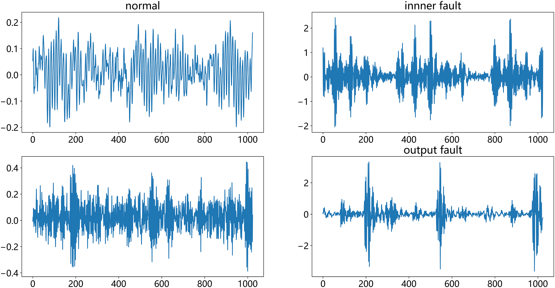
Figure 1: Fused signals

2.2 Markovian Transition Field

MTF is a time series image coding method based on the Markovian transfer matrix. In this paper, one-dimensional time signals are processed by MTF, and the acquired vibration signals are input into MTF and output as two-dimensional time series images. The image size is 224 × 224 and the Markov image transformation steps are as follows [27]:

1.   Division of data

Suppose the data is X∈[x1,x2,x3⋯xn] divided into U fractional-digit value domain intervals according to the range of values, and each xi corresponds to a qi,i∈[1,2,3⋯U]

2.   Construct the state transfer matrix D

Calculate the state transfer probability ωi,j based on the Markov chain principle to obtain a state transfer matrix D. The matrix size is [U,U].

ωi,j=∑∀,x∈qi,y∈qi,x+1=y1∑j=1Uωi,j,D=[ω11ω12⋯ω1Uω21ω22⋯ω2U⋮⋮⋱⋮ωU1ωU2⋯ωUU](9)

where ωi,j is the probability that the data in qi at moment t is transferred to qj at moment t + 1.

3.   Constructing Markovian transition field M

M=[ωi,j|x1∈qi,x1∈qjωi,j|x1∈qi,x2∈qj⋯ωi,j|x1∈qi,xn∈qjωi,j|x2∈qi,x1∈qjωi,j|x2∈qi,x2∈qj⋯ωi,j|x2∈qi,xn∈qj⋮⋮⋱⋮ωi,j|xn∈qi,x1∈qjωi,j|xn∈qi,x2∈qj⋯ωi,j|xn∈qi,xn∈qj](10)

There are three parameters in MTF that we need to select: image size, strategy, and bins, i.e., U. Image size determines information integrity. If the image is too small, information cannot be fully mapped to the image, leading to information loss. If the image is too large, it increases data volume and computational complexity, potentially introducing noise. Bins determine the degree of signal discretization. When the value is small, the signal is less discretized, resulting in a coarse image. When the value is large, each bin contains fewer data points, increasing data randomness and potentially introducing noise, while also increasing computational complexity. The most commonly used strategy is the position number strategy. The most commonly used strategy is the quantile strategy. We observe the resolvability of the generated images to obtain the optimal values. Below are the images generated by different parameters. The parameter selection is shown in Table 1. Fig. 2a–l shows a comparison of different MTF parameters.

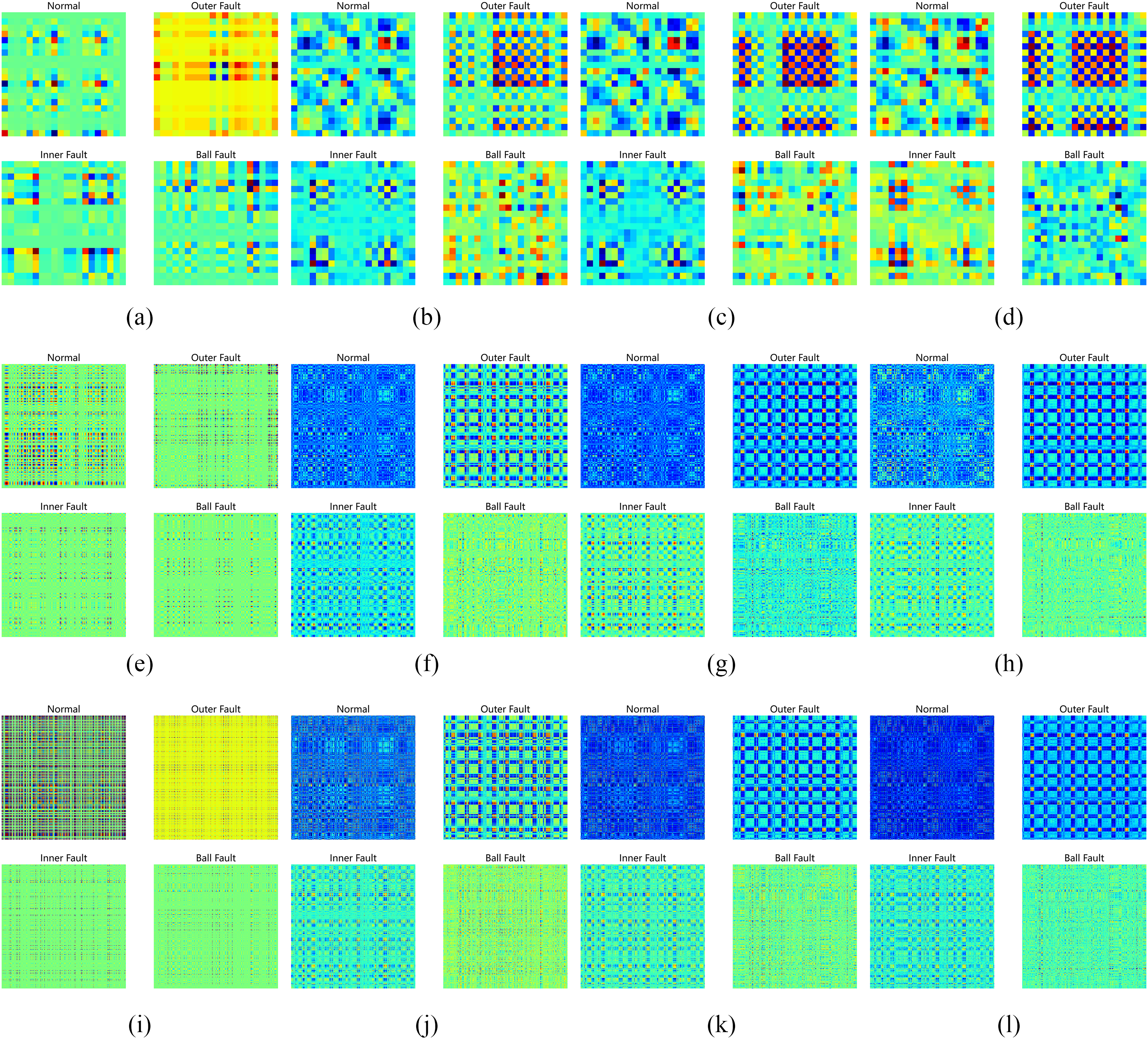
Figure 2: (a–l) MTF comparison chart

From the above view of the distinguishable degree of the images generated according to different parameters, the parameters of group (l) are better; therefore, the parameters selected for MTF in this paper are Image Size = 224, bins = 10, strategy = quantile.

2.3 Convolutional Neural Network

CNN, as a classical neural network, has been widely used in many disciplines due to its excellent performance. Since CNNs do not require preprocessing of the input image, they have attracted much attention in classification tasks [28]. The structure of CNN generally consists of an input layer, a convolutional layer, a pooling layer, a fully-connected layer, and an output layer, and Fig. 3 shows the structure of a CNN. The convolutional layer performs feature extraction on the input information by a convolution operation and enhances the features by an activation function. The convolution operation can be expressed as:

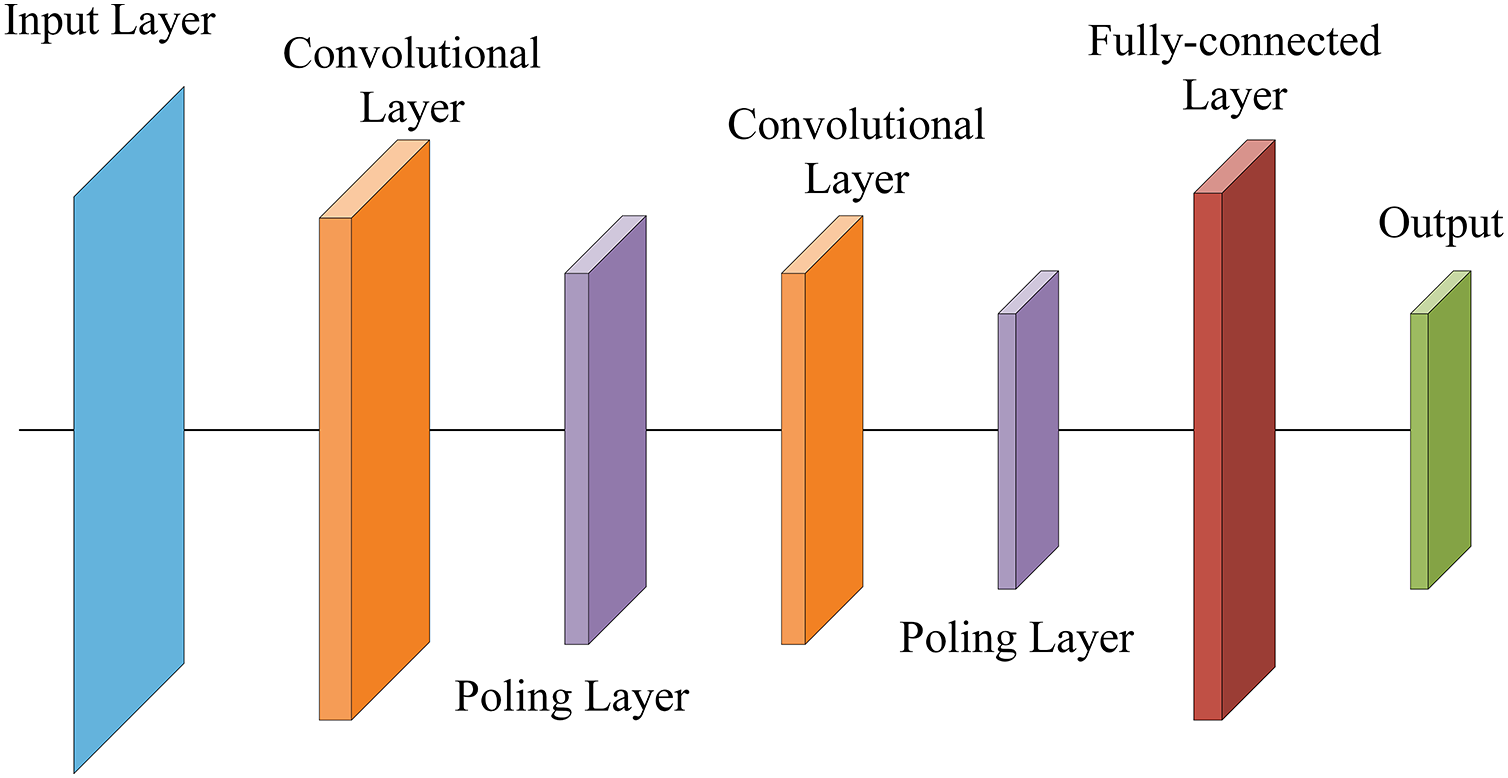
Figure 3: CNN structure

xil=f(∑j∈Mixil−1∗wjil+Bil)(11)

where xil is the i element of layer l; Mi is the ith convolution region of the feature map of layer l – 1; wjil is the weight matrix; Bil is the bias; and f is the activation function.

Pooling layers are generally placed after convolution layers and are further divided into max pooling and average pooling. Pooling reduces the subsequent computational load and parameter count while also reducing the risk of overfitting. Average pooling can be expressed as:

Mi,j=1c×c∑m=ism+c−1∑n=jsn+c−1Am,n(12)

Maximum pooling can be expressed as:

Mi,j=maxm=ism+c−1maxn=isn+c−1Am,n(13)

where Mi,j represents the corresponding element in the output feature map; c is the window size; m and n are both indices; and Am,n represents the corresponding element in the input feature map.

The fully connected layer (FC) integrates the local features from the previous multi-layer convolutions and pooling into global features. For classification tasks, FC maps the features to the category space for classification. FC can be represented as:

Y=f(Wx+b)(14)

where Y is the output; W is the weight; b is the bias.

2.4 Gated Recurrent Units

GRU is similar to a recurrent neural network and LSTM, which solves the problems of gradient vanishing and gradient explosion in back propagation and long-term memory in RNN. Unlike LSTM, it includes only an update gate and a reset gate, and is better able to capture long-time dependencies through a learnable gating mechanism. Fig. 4 shows the gating mechanism. The GRU gating principle steps are as follows [29]:

1.   Calculation update gate zt

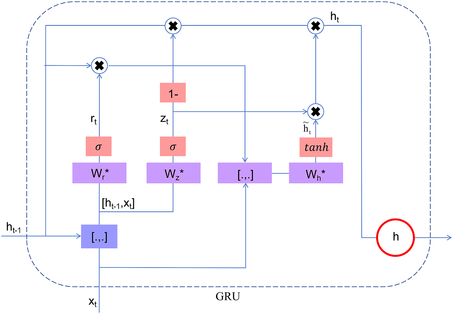
Figure 4: GRU gating mechanism

zt=σ(Wz⋅[ht−1,xt]+bz)(15)

2.   Calculation update gate rt

rt=σ(Wr⋅[ht−1,xt]+br)(16)

3.   Calculating Candidate Hidden States h~t

h~t=tanh⁡(Wh⋅[rt⋅ht−1,xt]+bh)(17)

where rt⋅ht−1 denotes the hidden state of the previous time step combined with the reset gate.

4.   Update hidden status ht

ht=zt⋅ht−1+(1−zt)⋅ht(18)

where zt⋅ht−1 denotes retained historical information and (1−zt)⋅h~t denotes new information.

2.5 Swin-Transformer

Swin-Transformer introduces a shift window based on Transformer to limit the scope of the window for self-attention computation and, simultaneously, allows cross-window connection, which improves the computational efficiency and reduces the complexity of the model itself. Swin-Transformer is a hierarchical structure, with the first layer consisting of a Split Layer, Linear Embedding Layer, Block Layer, and Merge Layer, and the Merge Layer and Block Layer are designated as a Stage. The Layer, Merge, and Block layers are designated as a Stage. Fig. 5 shows the structure of Swin-Transformer.

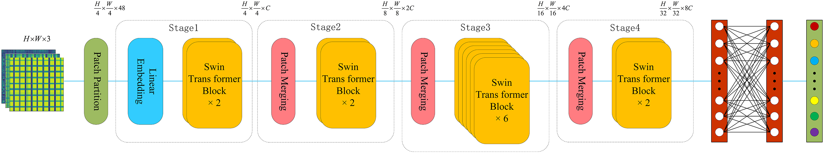
Figure 5: Swin-Transformer structure diagram

A Block consists of a W-MSA, SW-MSA, and a Multi-Layer Perceptron (MLP). Fig. 6 shows the Block layer structure. The Block computation can be represented as [13]:

z^l=W−MSA(LN(zl−1))+zl−1,zl=MLP(LN(z^l))+z^lz^l+1=SW−MSA(LN(zl))+zl,zl+1=MLP(LN(z^l+1))+z^l+1(19)

where z^l,zl are the S(W)-MSA output features and MLP output features of the first Block, respectively.

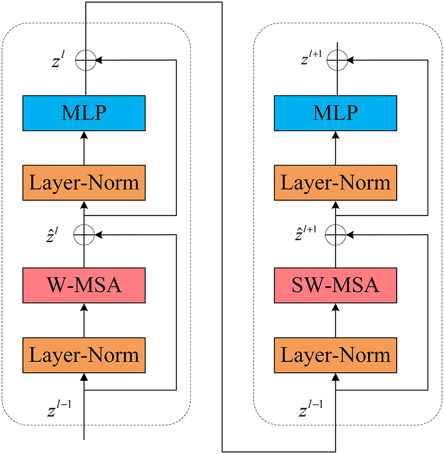
Figure 6: Block structure diagram

The structure of the multi-head attention mechanism (Multi Head Self Attention) in Swin-Transformer is shown in Fig. 7, and the computation can be represented as:

Attention(Q,K,V)=Softmax(QKTdk+B)V(20)

where Q,K,V is the query matrix, key matrix and value matrix respectively and B is the bias matrix.

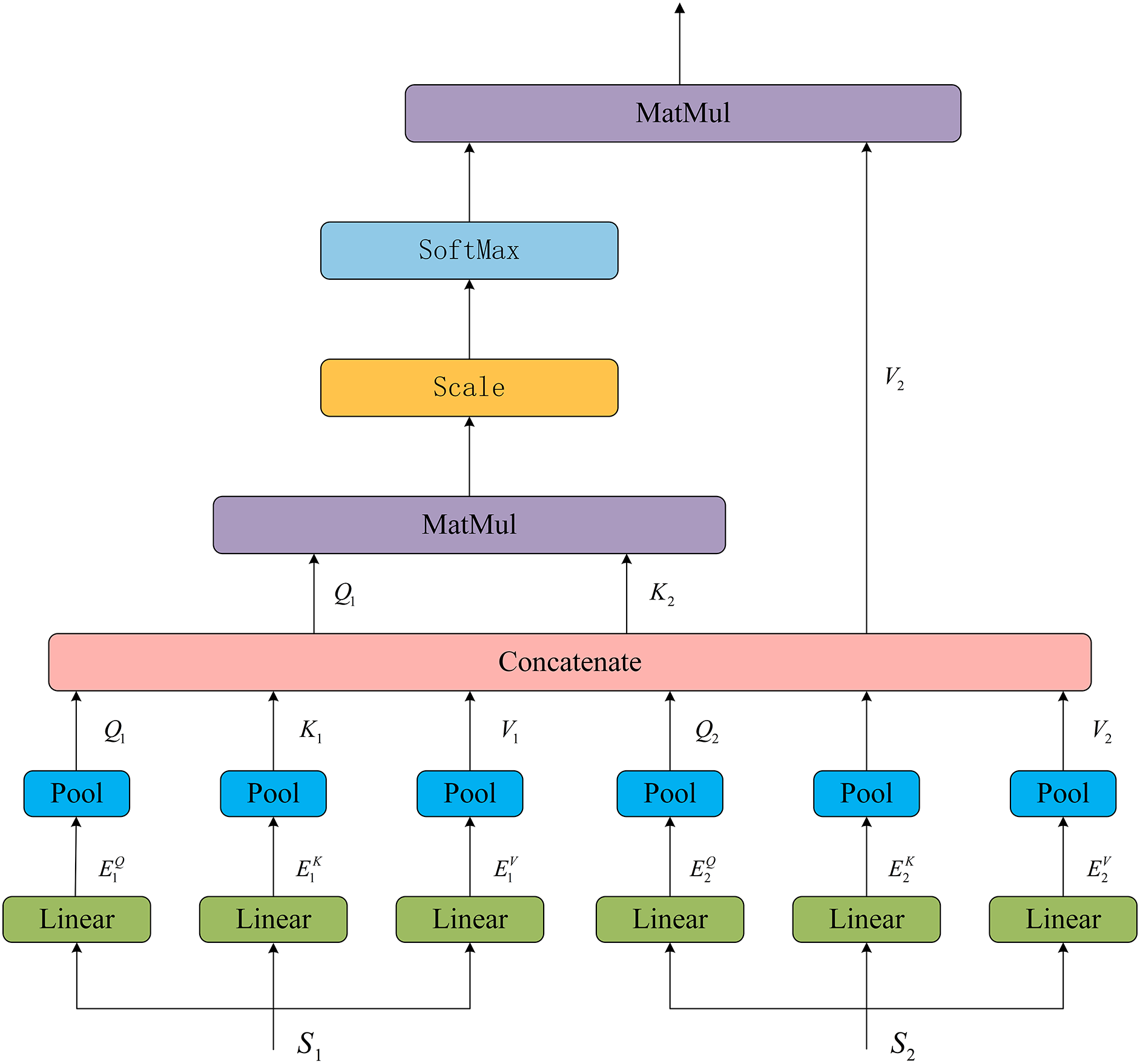
Figure 7: MSA structure

2.6 Convolution Block Attention Module

CBAM is a lightweight attention module. Fig. 8 shows the CBAM structure. The input feature maps will infer the attention maps sequentially along the channel attention and spatial attention, and finally multiply the attention features with the input feature maps for adaptive feature optimization.

Figure 8: CBAM model

The channel attention module performs pooling operation on the input feature map and then enters the shared layer to compress the dimensions, performs element-by-element summation and passes it to generate the channel attention map. Finally, the generated attention map is multiplied by the input feature map to get the channel feature map. Fig. 9 shows the channel attention module. The channel attention mechanism can be expressed as [12]:

Mc(F)=σ(MLP(Favgc)+MLP(Fmaxs)),Fc′=Mc(F)⊗F(21)

where Mc(F) is the output; F is the input; is the Sigmoid function; Favgc,Fmaxc is mean pooling and maximum pooling; FC1 is the channel feature map; and ⊗ denotes element-by-element multiplication.

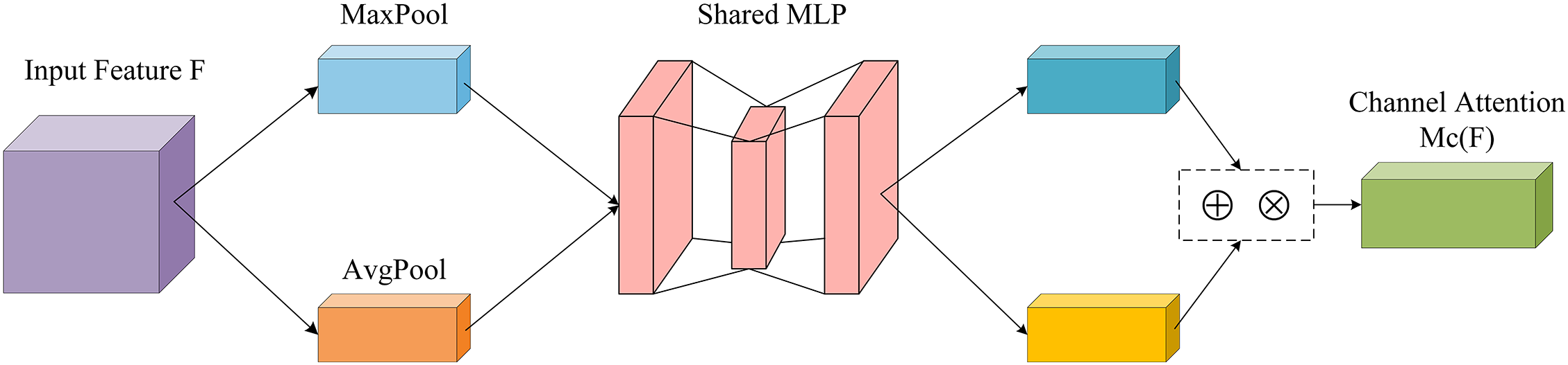
Figure 9: Channel attention model

The spatial attention module input comes from the channel attention output. Firstly, the input is subjected to average pooling and maximum pooling based on the channel dimensions, then spliced over the channel dimensions to get the feature maps, a 7 × 7 convolution operation is applied to the feature maps, and finally, the spatial attention maps are obtained σ. Finally, the input feature map is multiplied to get the spatial feature map. Fig. 10 shows the spatial attention module. The spatial attention module can be expressed as:

Ms(F)=σ(Conv7×7([Favgs,Fmaxs])),Fs′=Ms(F)⊗F(22)

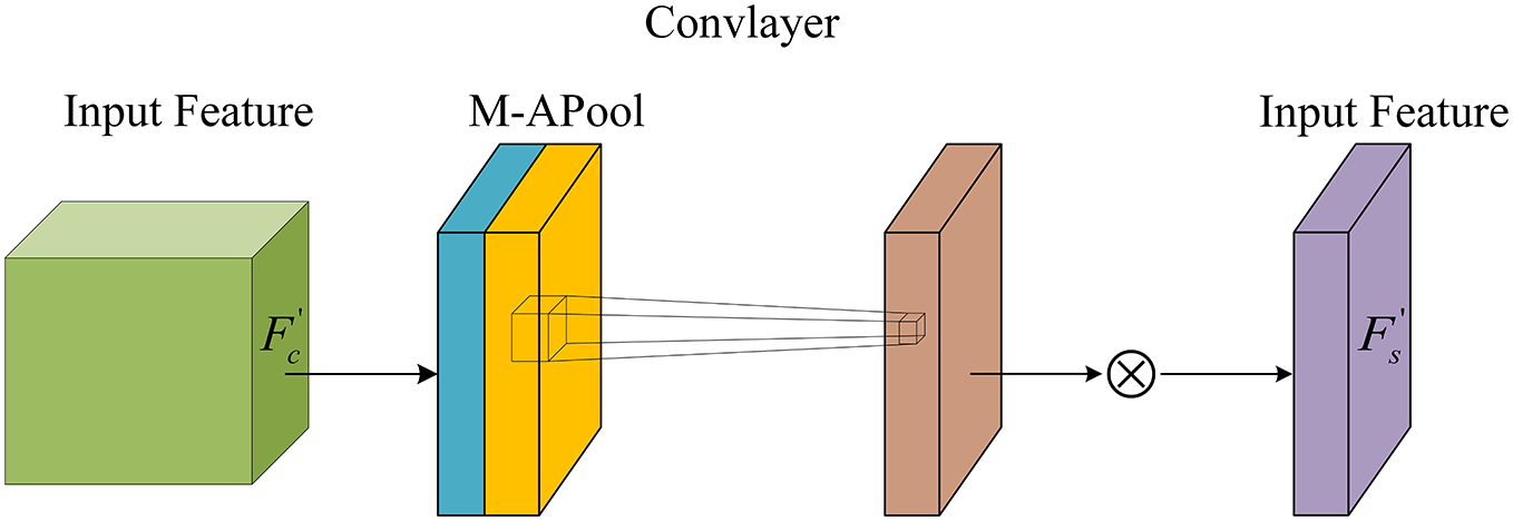
Figure 10: Space attention model

3  GSTCN Network Model

This paper proposes a multi-modal fault diagnosis model, GSTCN, and the network model structure is shown in Fig. 11. The model performs fault diagnosis in 3 steps: 1. Raw data processing stage; 2. Multimodal feature extraction stage; 3. Classification stage. The specific process is as follows:

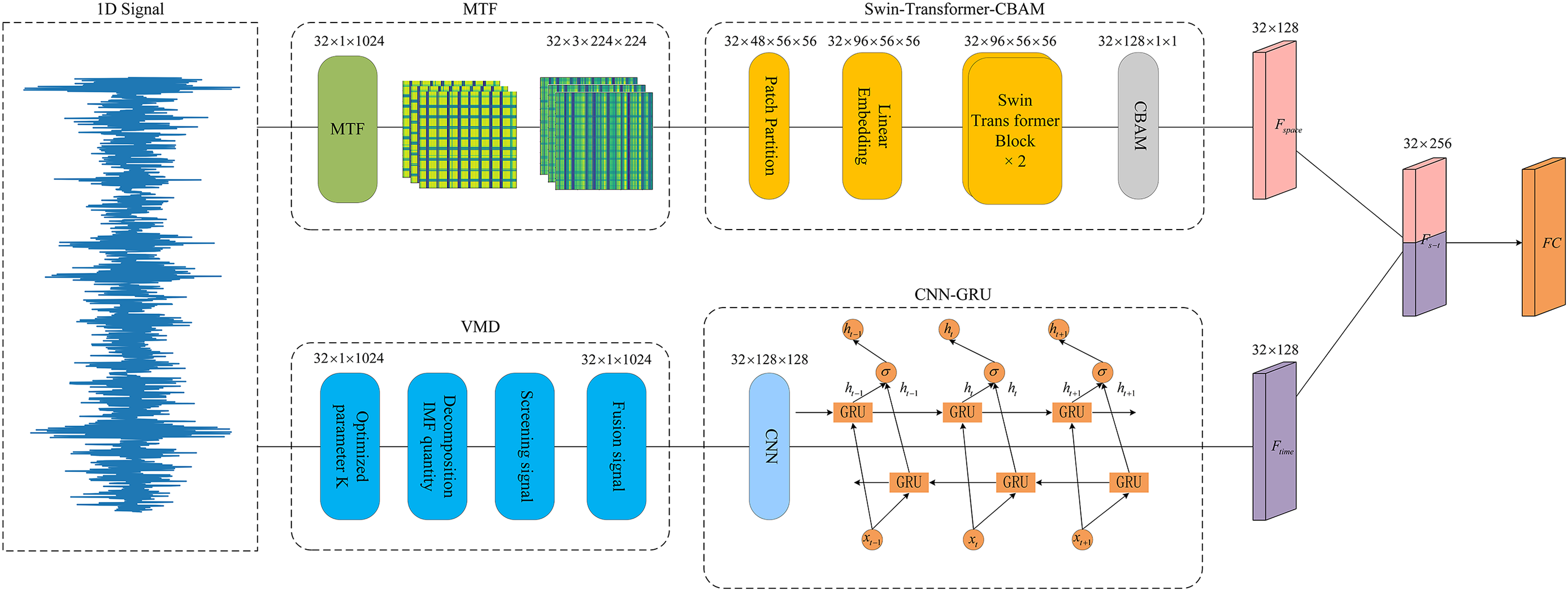
Figure 11: GSTCN network mode

1.    Bearing vibration data are collected by acceleration sensors, and the signals are processed into two-dimensional and one-dimensional signals to construct multimodal states by Markovian Transition Field and variational modal decomposition.

2.    The 2D data is extracted by Swin-Transformer to extract spatial features, then into CBAM to enhance the spatial features and output Fs, and the 1D data is extracted by the cyclic gating unit to extract temporal features Ft.

3.    The extracted time features and spatial features are fused into a single feature and finally fed into the classification layer for classification.

3.1 Original Signal Processing

Under complex operating conditions, one-dimensional time signals inevitably suffer from interference, leading to a decline in signal quality. Therefore, signal preprocessing is extremely important. This paper uses variational modal decomposition to reconstruct one-dimensional time series signals, restore fault signals, and fuse the reconstructed signals. Fig. 12 shows the variational modal decomposition signal and the fused signal. There are two key parameters in the variational modal decomposition, K and α, K determines how many IMF components are to be decomposed, and too large a number of modes will cause the signal to be over-decomposed, generating a number of spurious components and possibly introducing noise. Too small a number of modes can result in inadequate signal decomposition, losing some important information, leading to a reduction in the accuracy of the reconstructed signal. The reconstructed signal is closer to the original signal when the penalty factor is large, which retains the detailed information better, but may lead to overfitting. The smaller penalty factor allows for some error, which reduces the effect of noise to some extent, but may result in losing some of the detailed information. At the same time to take into account the problem of computing power consumption, thus in this paper, the variational modal decomposition selected α = 2000, the use of HO optimization algorithms to optimize the selection of the value of K, specifically through the Hilbert transform to calculate the most envelope entropy, select the value of entropy value of the smallest K value, the value of K range is k∈[1,10]. The signals were filtered using correlation coefficients and kurtosis to retain the components that were greater than 0.3 and with a kurtosis greater than three, and fused the components, or if there were no signals to satisfy this, the original signal was treated as a fused signal.

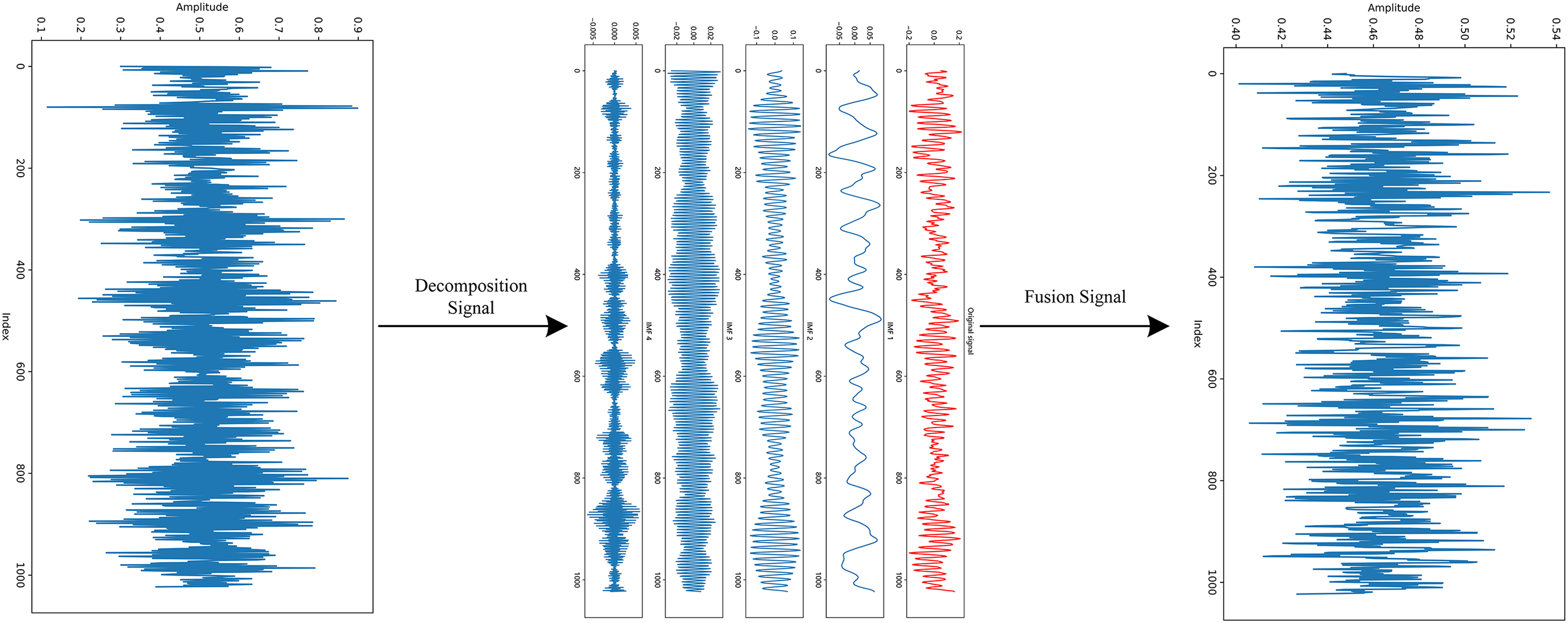
Figure 12: VMD signal processing

3.2 Multimodal Feature Extraction

The advantage of multimodal analysis is that it obtains fault characteristics from different dimensions to complement each other. First, the time series data is reconstructed using variational modal decomposition, and the signal shape is [1, 1024]. Then it enters the three-layer CNN. Each layer parameter is as follows: the size of the convolution kernel is 3×3; pooling adopts the maximal pooling, the pooling window is 2×2; and the step size is 2. The output features of the CNN enter into the GRU, which adopts a 2-layer structure with 64 neurons in each layer, and the parameters of the GRU are set to be as follows: number of hidden units 64; output feature shape is [32, 128]. One-dimensional data is converted into two-dimensional images after Markovian Transformer Field and input into Swin-Transformer, which is a one-layer structure, and the output features are augmented with spatial attention and channel attention of CBAM to enhance the fault features. The learning rate is 0.0001, the optimizer is Adam, and the batch size is 32. The dimensional changes and parameter configurations of the data passing through each module are shown in Table 2.

3.3 Feature classification

The features from the VMD and CNN-GRU branch outputs are used as Ftime, and the features from the MTF and Swin-Transformer-CBAM branch outputs are used as Fspace. Then, Ftime and Fspace are concatenated along the dimension direction to form a signal that is fed into the FC layer for feature classification.

4  Experiments and Results

In this section, experiments are conducted using the Case Western Reserve University (CWRU) dataset, the Jiangnan University dataset, and a simulated dataset to compare the performance of the proposed model and validate its generalization and accuracy. Evaluation metrics typically include accuracy, precision, recall, and F1-score, which help assess the model’s effectiveness and the impact of hyperparameters. Additionally, runtime and parameter count are included. Runtime is calculated by measuring the total training time for one round, while parameter count refers to the total number of parameters in the current model. For the model’s classification performance, we use a confusion matrix for evaluation, which describes the proportion or number of correct or incorrect classifications in each category, effectively assessing the model’s classification performance.

The experimental platform configuration is as follows: CPU i7-13400H; RAM 16 G; GPU RTX4060; Python (V3.11.7) deep learning framework for model training and experimental validation.

4.1 Experiments and Results

The CWRU data set includes inner ring faults, outer ring faults, and rolling element faults, each with 7, 14, and 21 fault sizes, plus normal, together constituting a decile file, and the bearing vibration signals are collected using a 12 KHz frequency. The length of each sample data is 1024, and the overlap rate is set to 0.5. The training set, validation set, and test set are divided according to 7:3:1. Table 3 presents the CWRU data set.

The performance of the proposed model is verified by the Western Reserve University data set, and the classification is significant as can be seen from the confusion matrix. Fig. 13 shows the confusion matrix and classification visualization; Table 4 shows the evaluation metrics.

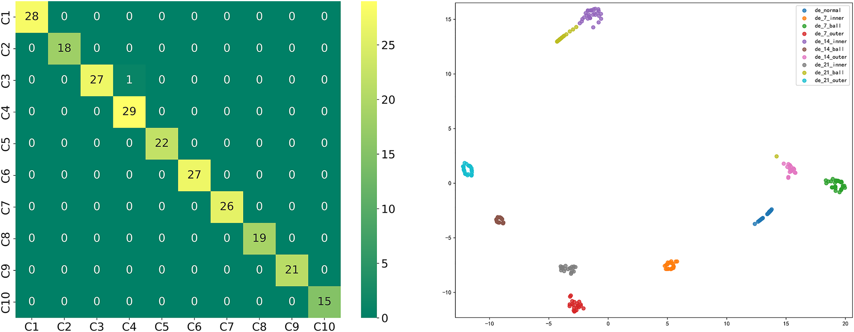
Figure 13: Confusion matrix and classification visualization

Control Experiment

Table 5 demonstrates the evaluation metrics of the compared models. Temporal convolutional network (TCN) uses convolutional operations for parallel computation and can effectively capture local dependencies, less prone to gradient problems. TCN-LSTM and CNN-GRU are used as traditional models for comparison. Zou et al. use three image transformation methods to transform a 1D signal into a 2D picture and augment it with the Kolmogorov-Arnold representation theorem. Residual network was used for cross-case diagnosis, and the effectiveness of the model was verified on two datasets [30]. Tong et al. designed an MTF-based combined hybrid attention mechanism and residual network (MARN) for data imbalance and instability, and finally, the method was verified to achieve better diagnostic performance on the dataset [31]. Fig. 14a–d shows the confusion matrix for comparing the models.

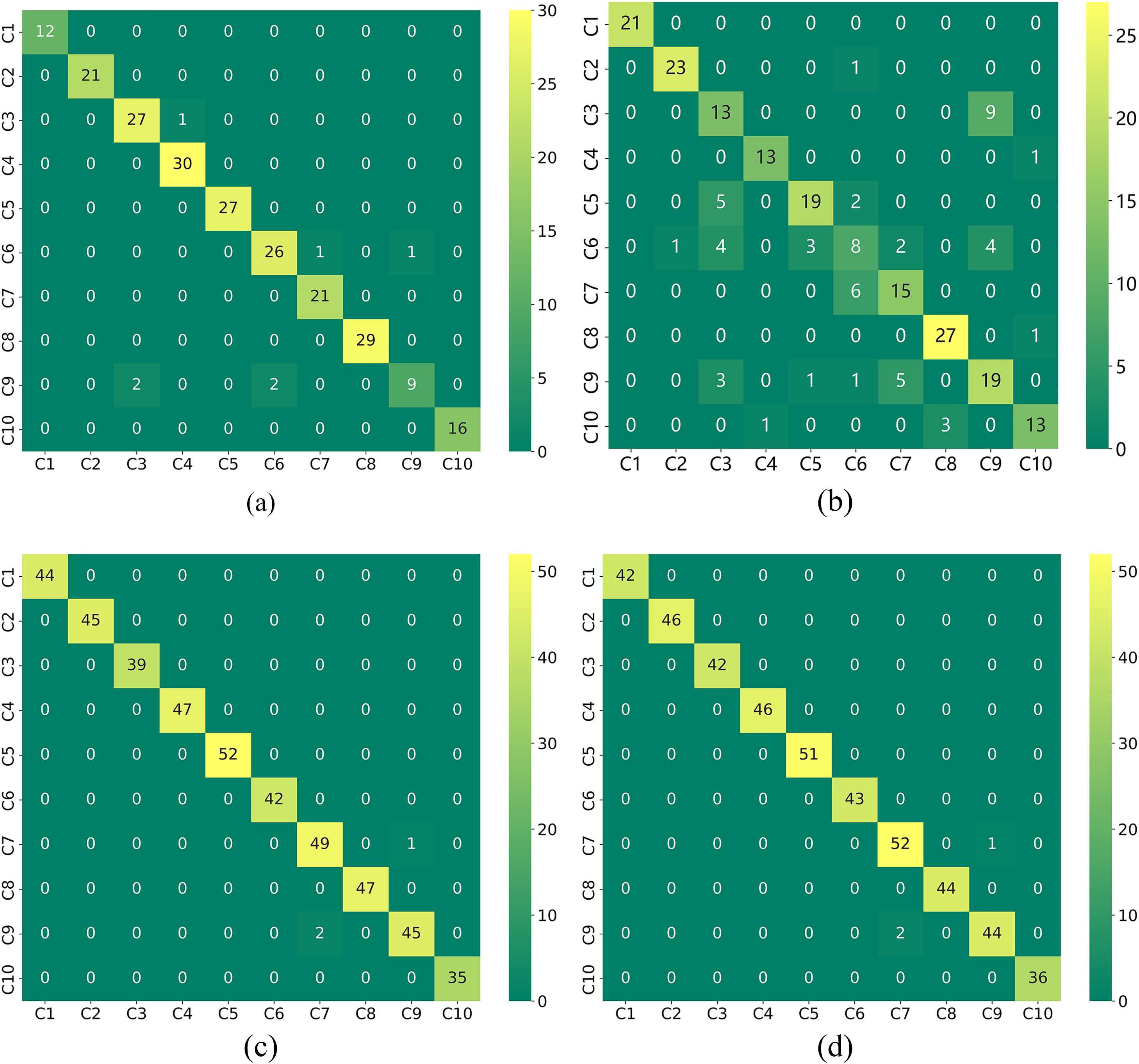
Figure 14: The confusion matrix for the comparison model. (a) CNN; (b) TCN; (C) MKA; (d) MTF

4.2 Simulated Bearing Data

The dataset was sampled at 20 KHz and used 6007 deep groove ball bearings at 1500 r/min. pitting was used to simulate the faulty bearings. The outer ring failure, rolling element failure, inner ring failure, and normal condition together constitute four classification files. Table 6 describes the simulation experiment data set. The simulation experiment platform is shown in Fig. 15.

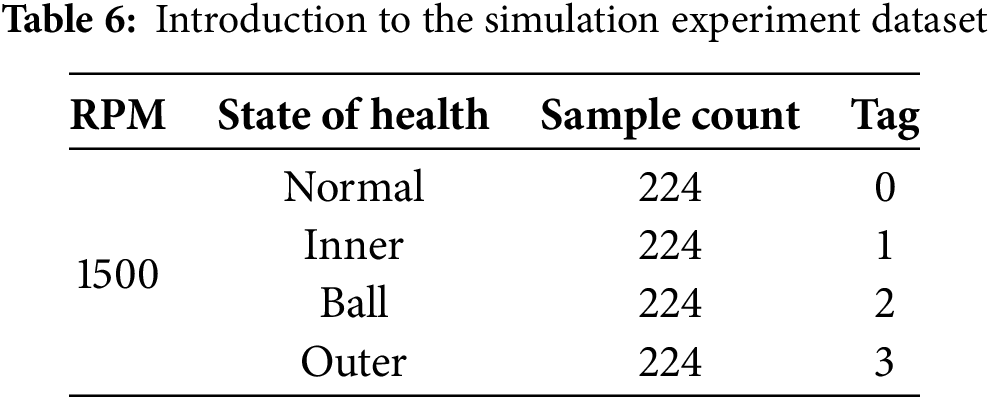
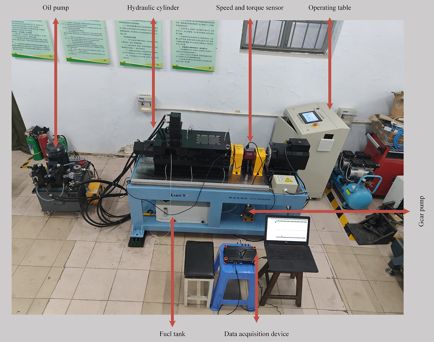
Figure 15: Bearing test platform

After validation with simulated experimental data, the model still exhibits high classification accuracy and good generalization ability. Fig. 16 shows the confusion matrix and classification visualization; Table 7 lists the evaluation metrics.

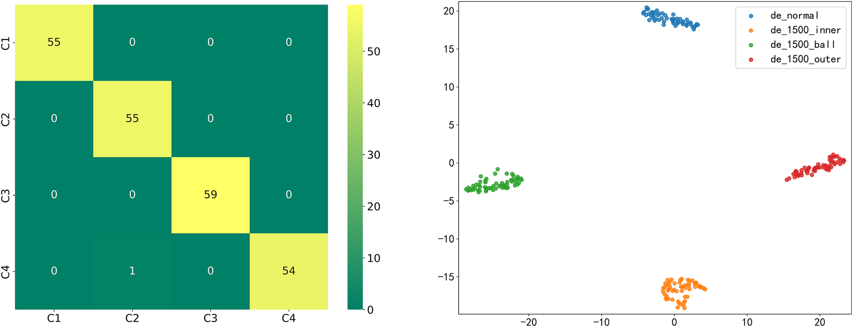
Figure 16: Confusion matrix and classification visualization

Control Experiment

Simulated experimental data were compared using traditional models. Fig. 17 shows the confusion matrices, and Table 7 shows the model comparison table.

Figure 17: Confusion matrix: left CNN, right TCN

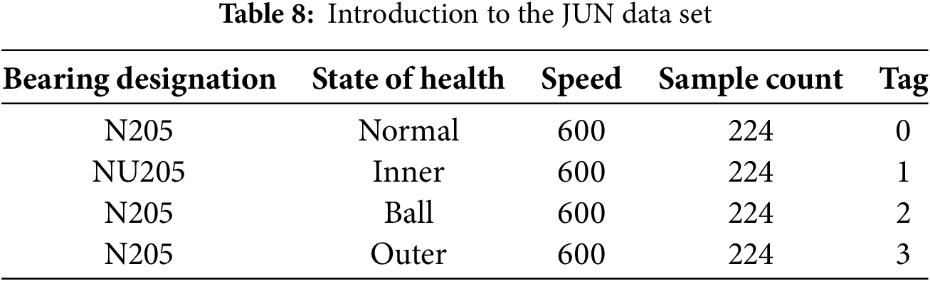
4.3 JUN Bearing Experimental Data

Jiangnan University dataset (JNU) sampling frequency 50 KHz using bearing type N205 and NU205 two types, which are normal, outer ring failure, and rolling body failure using N205, inner ring failure using separable NU205. Each type of failure to take the 600 rpm rotational speed of the state constitutes a four-classification file, Table 8 for the introduction of the JUN data set.

After JNU experimental data validation, the model classification effect is significant. Fig. 18 shows the confusion matrix and classification visualization; Table 9 shows the evaluation metrics.

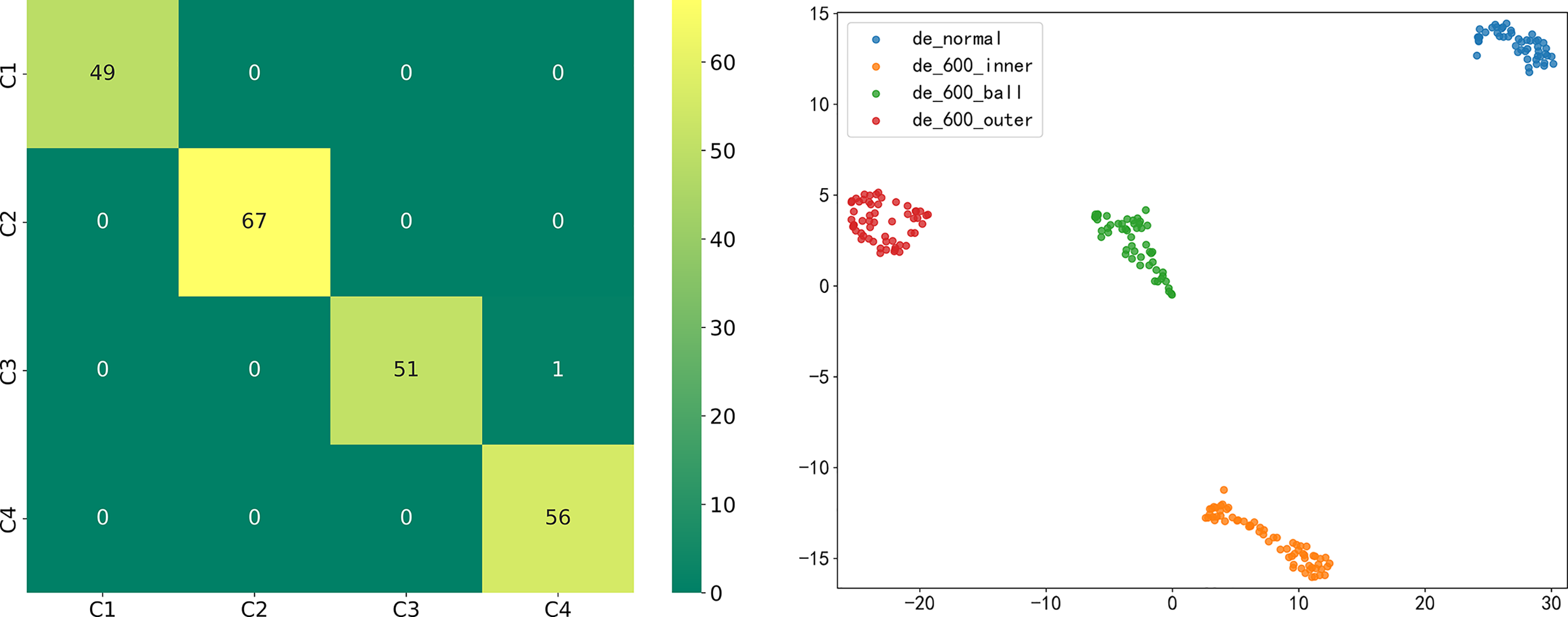
Figure 18: Confusion matrix and categorical visualization

Control Experiment

Wei et al. used Continuous Wavelet Transform (CWT) to process the original signals and proposed a parallel neural network by adding channel attention to the CNN in conjunction with BiLSTM and residuals. The network showed good diagnostic performance [32]. Xu et al. designed a Multi-branch Dynamic Convolutional Network (MBDCNet), which was used for a fault diagnosis method in migration learning by changing the traditional convolution to dynamic convolution. Experimental results show that the method has good stability in diagnostic tasks [33]. Fig. 19a–d shows the confusion matrix, and Table 10 shows the model comparison table.

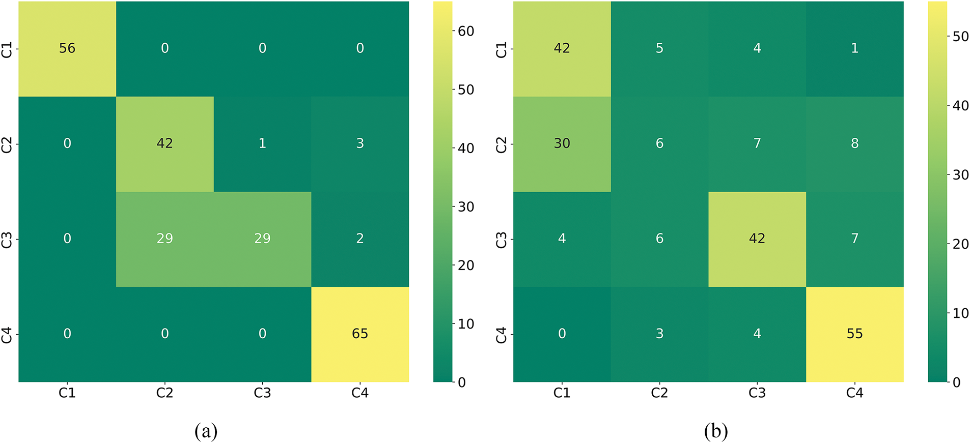
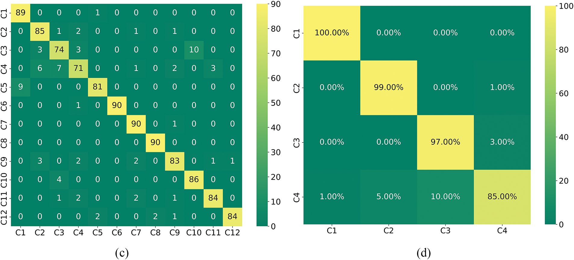
Figure 19: The confusion matrices of the comparison models. (a) CNN; (b) TCN; (c) CWT; (d) MBDCNet

4.4 JNU Ablation Experiment

To better understand the contribution of each module in the model, we conducted ablation experiments on the model using the Jiangnan University dataset. The specific ablation experiment models are shown in Table 11. Model-1 and Model-2 lack VMD, Model-2 lacks the two-dimensional data extraction branch and only includes the one-dimensional data extraction processing module, Model-3 lacks CBAM compared to Model-4, Model-4 lacks the one-dimensional data extraction branch and only includes the two-dimensional data extraction processing module, Model-5 lacks CBAM, and Model-6 lacks GRU. Since MTF and VMD do not involve parameter quantity issues, only the runtime for a single signal is provided. MTF processing a single signal takes 52 ms, and VMD processing a single signal takes 410 ms. Table 12 shows the evaluation metrics, and Fig. 20a–f displays the confusion matrices.

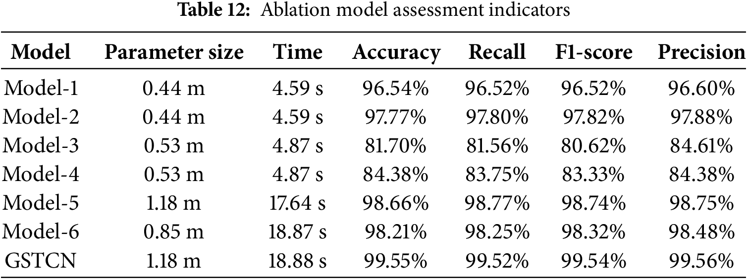
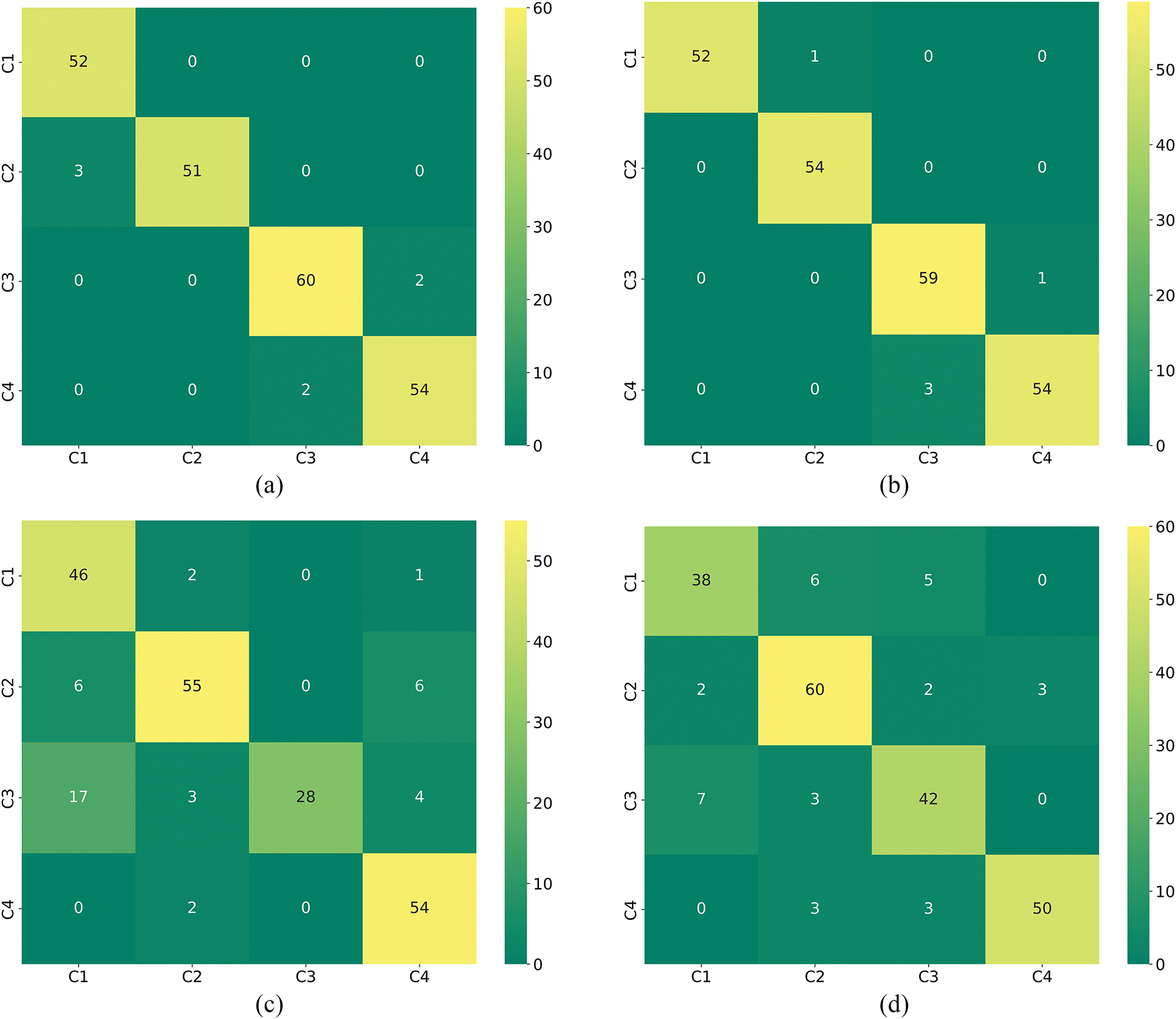
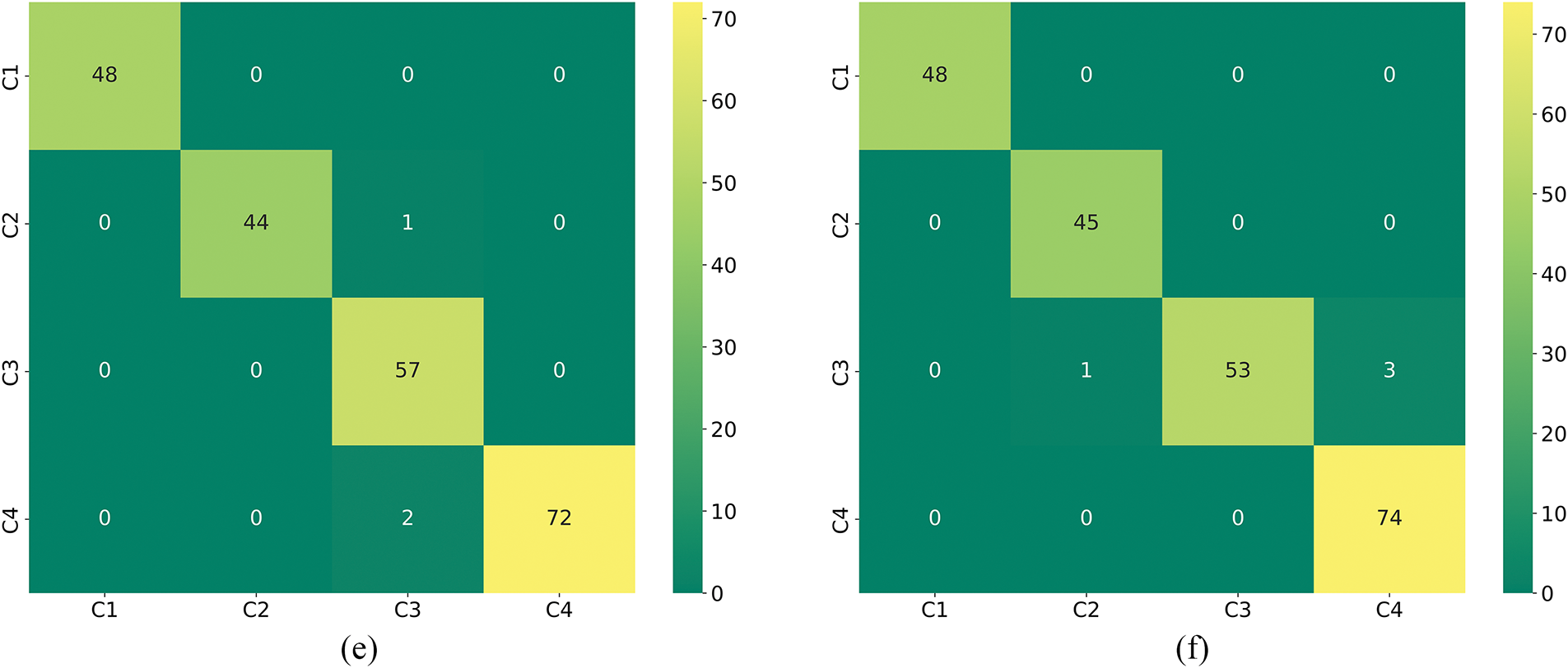
Figure 20: The confusion matrix of the ablation Models (1–6) correspond to (a–f)

To evaluate how the CBAM attention mechanism helps the model better focus on fault areas, the attention mechanism was visualized using a heat map. As shown in Fig. 21, the attention level of the fault area is significantly higher than that of other areas, proving the effectiveness of CBAM.

Figure 21: Attention mechanism heat map

The above ablation experiments can be obtained that VMD improves the signal quality to enhance the diagnostic effect, and the addition of CBAM enhances the extracted fault features. The above ablation experiments indicate that the combination of a single modality improves the complexity of the model and indeed helps to improve the model performance and classification accuracy, but due to the inability of a single modality to extract the complete information leads to the existence of a small number of samples are still confusing, and when the model is too complex, it requires a significant increase in the arithmetic resources and also increases the risk of overfitting. Therefore, the advantages of the model studied in this paper are significant.

5  Conclusion

The GSTCN multimodal fusion fault diagnosis method proposed in this paper is summarized as follows: The Ho optimization algorithm combined with the minimum envelope entropy criterion achieves adaptive selection of the number of VMD modes. Meanwhile, the signal is reconstructed using correlation coefficients and kurtosis indicators, laying a high-quality data foundation for subsequent time-series feature extraction. CBAM is introduced after Swin-Transformer, enabling the model to dynamically prioritize key regions associated with faults. Test results on three bearing datasets—CWRU, Jiangnan University (JUN), and simulated experiments—show that the GSTCN model achieves an average accuracy rate of 99.5%, significantly outperforming traditional methods. In real-world machine operations, bearing fault data is scarce, and the number of samples collectible during a fault event is limited. Therefore, future research should focus on developing fault diagnosis methods for small sample sizes to provide stronger safety guarantees for operators.

Acknowledgement: Not applicable.

Funding Statement: This research was funded by the Jilin Provincial Department of Science and Technology, grant number 20230101208JC.

Author Contributions: Concept, Yingyong Zou and Yu Zhang; Methodology, Yingyong Zou and Yu Zhang; Resources, Yingyong Zou; Data Management: Long Li; Writing—Drafting: Yu Zhang; Writing—Reviewing and Editing: Yingyong Zou, Long Li and Yu Zhang; Supervision: Tao Liu and Xingkui Zhang; Project Management: Yingyong Zou; Funding Acquisition: Yingyong Zou. All authors reviewed the results and approved the final version of the manuscript.

Availability of Data and Materials: The datasets covered in this thesis are publicly available from [https://engineering.case.edu/bearingdatacenter/download-data-file (accessed on 9 September 2025)];[https://github.com/ClarkGableWang/JNU-Bearing-Dataset (accessed on 9 September 2025)].

Ethics Approval: Thanks to Jilin Provincial Department of Science and Technology.

Conflicts of Interest: The authors declare no conflicts of interest to report regarding the present study.

References

1. Wang L, Zhao W. An ensemble deep learning network based on 2D convolutional neural network and 1D LSTM with self-attention for bearing fault diagnosis. Appl Soft Comput. 2025;172(4):112889. doi:10.1016/j.asoc.2025.112889. [Google Scholar] [CrossRef]

2. Zhan F, Hu L, Huang W, Dong Y, He H, Wu G, et al. Category knowledge-guided few-shot bearing fault diagnosis. Eng Appl Artif Intell. 2024;139(4):109489. doi:10.1016/j.engappai.2024.109489. [Google Scholar] [CrossRef]

3. Li Y, Cheng G, Liu C. Research on bearing fault diagnosis based on spectrum characteristics under strong noise interference. Measurement. 2021;169(1):108509. doi:10.1016/j.measurement.2020.108509. [Google Scholar] [CrossRef]

4. Zhao K, Xiao J, Li C, Xu Z, Yue M. Fault diagnosis of rolling bearing using CNN and PCA fractal based feature extraction. Measurement. 2023;223(8):113754. doi:10.1016/j.measurement.2023.113754. [Google Scholar] [CrossRef]

5. Ruan D, Wang J, Yan J, Gühmann C. CNN parameter design based on fault signal analysis and its application in bearing fault diagnosis. Adv Eng Inform. 2023;55(1):101877. doi:10.1016/j.aei.2023.101877. [Google Scholar] [CrossRef]

6. Encalada-Dávila Á, Moyon L, Tutivén C, Puruncajas B, Vidal Y. Early fault detection in the main bearing of wind turbines based on gated recurrent unit (GRU) neural networks and SCADA data. IEEE/ASME Trans Mechatron. 2022;27(6):5583–93. doi:10.1109/tmech.2022.3185675. [Google Scholar] [CrossRef]

7. Li X, Su H, Xiang L, Yao Q, Hu A. Transformer-based meta learning method for bearing fault identification under multiple small sample conditions. Mech Syst Signal Process. 2024;208(12):110967. doi:10.1016/j.ymssp.2023.110967. [Google Scholar] [CrossRef]

8. Chen L, Yao H, Fu J, Ng C. The classification and localization of crack using lightweight convolutional neural network with CBAM. Eng Struct. 2023;275:115291. doi:10.1016/j.engstruct.2022.115291. [Google Scholar] [CrossRef]

9. Kansal S, Jha S, Samal P. DL-DARE: deep learning-based different activity recognition for the human-robot interaction environment. Neural Comput Appl. 2023;35(16):12029–37. doi:10.1007/s00521-023-08337-y. [Google Scholar] [CrossRef]

10. Xu Z, Li C, Yang Y. Fault diagnosis of rolling bearings using an improved multi-scale convolutional neural network with feature attention mechanism. ISA Trans. 2021;110(3):379–93. doi:10.1016/j.isatra.2020.10.054. [Google Scholar] [PubMed] [CrossRef]

11. Liu L, Wang Y, Chi W. Image recognition technology based on machine learning. IEEE Access. 2020;1. doi:10.1109/ACCESS.2020.3021590. [Google Scholar] [CrossRef]

12. Praharsha CH, Poulose A. CBAM VGG16: an efficient driver distraction classification using CBAM embedded VGG16 architecture. Comput Biol Med. 2024;180(14):108945. doi:10.1016/j.compbiomed.2024.108945. [Google Scholar] [PubMed] [CrossRef]

13. Zhou K, Lu N, Jiang B, Ye Z. FEV-Swin: multi-source heterogeneous information fusion under a variant swin transformer framework for intelligent cross-domain fault diagnosis. Knowl Based Syst. 2025;310(3):112982. doi:10.1016/j.knosys.2025.112982. [Google Scholar] [CrossRef]

14. Gong T, Li S, Zhang Y, Zhou L, Xia M. Digital twin-assisted intelligent fault diagnosis for bearings. Meas Sci Technol. 2024;35(10):106128. doi:10.1088/1361-6501/ad5f4c. [Google Scholar] [CrossRef]

15. Niu J, Pan J, Qin Z, Huang F, Qin H. Small-sample bearings fault diagnosis based on ResNet18 with pre-trained and fine-tuned method. Appl Sci. 2024;14(12):5360. doi:10.3390/app14125360. [Google Scholar] [CrossRef]

16. Cheng J, Qi H, Ma R, Kong X, Zhang Y, Zhu Y. FS-PTL: a unified few-shot partial transfer learning framework for partial cross-domain fault diagnosis under limited data scenarios. Knowl Based Syst. 2024;305(3):112658. doi:10.1016/j.knosys.2024.112658. [Google Scholar] [CrossRef]

17. Zhang L, Zhang J, Peng Y, Lin J. Intra-domain transfer learning for fault diagnosis with small samples. Appl Sci. 2022;12(14):7032. doi:10.3390/app12147032. [Google Scholar] [CrossRef]

18. Zhao B, Zhang X, Li H, Yang Z. Intelligent fault diagnosis of rolling bearings based on normalized CNN considering data imbalance and variable working conditions. Knowl Based Syst. 2020;199:105971. doi:10.1016/j.knosys.2020.105971. [Google Scholar] [CrossRef]

19. Lal S, Van Khang H, Robbersmyr KG. Multiple classifiers and data fusion for robust diagnosis of gearbox mixed faults. IEEE Trans Ind Inform. 2019;15(8):4569–79. doi:10.1109/tii.2018.2883357. [Google Scholar] [CrossRef]

20. Guo Y, Hu T, Zhou Y, Zhao K, Zhang Z. Multi-channel data fusion and intelligent fault diagnosis based on deep learning. Meas Sci Technol. 2022;34(1):015115. doi:10.1088/1361-6501/ac8a64. [Google Scholar] [CrossRef]

21. Xu Z, Yang P, Zhao Z, Lai CS, Lai LL, Wang X. Fault diagnosis approach of main drive chain in wind turbine based on data fusion. Appl Sci. 2021;11(13):5804. doi:10.3390/app11135804. [Google Scholar] [CrossRef]

22. Jiao J, Zhao M, Lin J-B, Ding C. Deep coupled dense convolutional network with complementary data for intelligent fault diagnosis. IEEE Trans Ind Electron. 2019;66(12):9858–67. doi:10.1109/tie.2019.2902817. [Google Scholar] [CrossRef]

23. Wang J, Lv X, Xu Y, Wan Y, Bao H, Han B. A novel subdomain adaptive intelligent fault diagnosis method based on multiscale adaptive residual networks. Meas Sci Technol. 2024;35(7):076112. doi:10.1088/1361-6501/ad3b2f. [Google Scholar] [CrossRef]

24. Li X, Ma Z, Kang D, Li X. Fault diagnosis for rolling bearing based on VMD-FRFT. Measurement. 2020;155(12):107554. doi:10.1016/j.measurement.2020.107554. [Google Scholar] [CrossRef]

25. Sun Y, Li S, Wang X. Bearing fault diagnosis based on EMD and improved Chebyshev distance in SDP image. Measurement. 2021;176(17):109100. doi:10.1016/j.measurement.2021.109100. [Google Scholar] [CrossRef]

26. Li H, Wu X, Liu T, Li S, Zhang B, Zhou G, et al. Composite fault diagnosis for rolling bearing based on parameter-optimized VMD. Measurement. 2022;201(5):111637. doi:10.1016/j.measurement.2022.111637. [Google Scholar] [CrossRef]

27. He K, Xu Y, Wang Y, Wang J, Xie T. Intelligent diagnosis of rolling bearings fault based on multisignal fusion and MTF-ResNet. Sensors. 2023;23(14):6281. doi:10.3390/s23146281. [Google Scholar] [PubMed] [CrossRef]

28. Wang H, Xu J, Yan R, Gao RX. A new intelligent bearing fault diagnosis method using SDP representation and SE-CNN. IEEE Trans Instrum Meas. 2020;69(5):2377–89. doi:10.1109/tim.2019.2956332. [Google Scholar] [CrossRef]

29. Yin S, Chen Z. Research on compound fault diagnosis of bearings using an improved DRSN-GRU dual-channel model. IEEE Sens J. 2024;24(21):35304–35. doi:10.1109/jsen.2024.3462540. [Google Scholar] [CrossRef]

30. Tang Z, Hou X, Wang X, Zou J. A cross-working condition-bearing diagnosis method based on image fusion and a residual network incorporating the Kolmogorov-Arnold representation theorem. Appl Sci. 2024;14(16):7254. doi:10.3390/app14167254. [Google Scholar] [CrossRef]

31. Tong A, Zhang J, Wang D, Xie L. Intelligent fault diagnosis of rolling bearings based on Markov transition field and mixed attention residual network. Appl Sci. 2024;14(12):5110. doi:10.3390/app14125110. [Google Scholar] [CrossRef]

32. Fu G, Wei Q, Yang Y, Li C. Bearing fault diagnosis based on CNN-BiLSTM and residual module. Meas Sci Technol. 2023;34(12):125050. doi:10.1088/1361-6501/acf598. [Google Scholar] [CrossRef]

33. Yin Z, Zhang F, Xu G, Han G, Bi Y. Multi-scale rolling bearing fault diagnosis method based on transfer learning. Appl Sci. 2024;14(3):1198–8. doi:10.3390/app14031198. [Google Scholar] [CrossRef]